Water Requirements (Chapter 6)

6

WATER REQUIREMENTS

by R. D. Burman, University of Wyoming. Laramie, WY; P. R. Nixon, USDA-SEA/AR, Weslaco, TX; J. L. Wright, USDA-SEA/AR, Kimberly, ID; and W. 0. Pruitt, University of California, Davis, CA

6.1 INTRODUCTION

The main objective of irrigation is to provide plants with sufficient water to prevent stress that may cause reduced yield or poor quality of harvest (Haise and Hagan, 1967; Taylor, 1965). The required timing and amount of applied water is governed by the prevailing climatic conditions, crop and stage of growth, soil moisture holding capacity, and the extent of root development as determined by type of crop, stage of growth, and soil.

Need for irrigation can be determined in several ways that do not require knowledge of evapotranspiration (ET) rates. One way is to observe crop in-dicators such as change of color or leaf angle, but this information may ap-pear too late to avoid reduction in crop yield or quality. This method has been used successfully with some crops like beans (liaise and Hagan, 1967). Other similar methods of scheduling, which involve determining the plant water stress, soil moisture status, or soil water potential are described in Chapter 18.

This chapter describes methods of estimating crop water requirements expressed as equivalent depth of water over the horizontal p rivet .on of the crop growing area This information, when combined with soil water holding characteristics, has the advantage of not only being useful in determining when to irrigate, but also enables specifying how much water to apply. Er in-formation is also needed in determining the volume of water required to satisfy short-term and seasonal water requirements for fields, farms and ir-rigation projects, and in designing water storage and distribution systems. In addition, this information is essential for most water right transfers from agriculture to other uses because most such transfers are limited to historic crop water use amounts.

Water use measurements have been made in many field experiments and at many locations. The data available from various sources are of varying quality depending upon the conditions and techniques that were used. The material presented in this chapter emphasizes methods of estimating ET rates and provides guidelines for estimating irrigation water requirements.

6.2. IMPORTANT DEFINITIONS

DL,516;r4 AND OPLIU, SION OF E'AltM ilitiliiAnUN S.C.:, ELMS WA 1E1i ilLULEIEE.LMCIA 1 S

6.2.1 Eiapotranspiration and Potential Evapotranspiration

The definition of evapotranspiration, abbreviated ET or symbolically E„ presented in this chapter is in widespread use. The definition of potential ET (E„.) is controversial and may have different meanings in various parts of the world and to different people in the same country. The following definitions include several variations of potential ET.

Evaptranspiration. The combined process by which water is transferred from the earth's surface to the atmosphere. It includes evaporation of liquid or solid water from soil and plant surfaces plus transpiration of liquid water through plant tissues expressed as the latent heat transfer per unit area or its equivalent depth of water per unit area.

Potential evapotranspiration. The rate at which water, if available, would be removed from the soil and plant surface expressed as the latent heat transfer per unit area or its equivalent depth of water per unit area.

Other definitions of potential evaptranspiration. Mathematically, in the common derivation of the combination equation, potential ET is the ET that occurs When the vapor pressure at the evaporating surface is at the saturation point (van Bavel. 1966). This definition is not limited to any particular degree of vegetation or growth stage of a crop. Since this definition is not restricted to a standard surface, it has had limited direct use by the designer or operator of an irrigation system.

Some investigators in the Western United States have used the ET from a well-watered crop like alfalfa with 30 to 50 cm of top growth and at least 100 in of fetch as representing potential ET (Jensen, 1974). Others have used ET from well-watered clipped grass as a potential ET. The height of the grass has been historically uncertain. Penman (1948) used clipped grass similar to a lawn to develop his version of the combination equation. Recently, this has been defined as "the rate of evapotranspiration from an extensive surface of 8- to 15-cm, green grass cover of uniform height, actively growing, complete-ly shading the ground, and not short of water" (Doorenbos and Pruitt, 1977). In testing the Penman formula, Makkink (1957) found that the height of the grass did have an influence on the ET rate.

Crop versus potential ET. The realtionship between the ET of a specific crop (E,) at a specific time in its growth stage and potential ET is of practical interest to the designer or operator of an irrigation system because ET estimates are often made from potential ET (E,d. The relationship has lead to crop coefficients:

K = E t

c [6./

Et P '

where K. is referred to as a crop coefficient incorporating the effects of crop growth stage, crop density, and other cultural factors affecting ET. Crop coefficients are discussed in more detail in Section 6.5. The crop coefficient defined in equation 16.11 _{is not the K factor used in the original} Blaney-Criddle method.

6.2.2 Reference Crop Evapotranspiration

Because of the ambiguities involved in the interpretation of potential evapotranspiration, the term "Reference Crop Evapotranspiration," or E„, is frequently being used, Doorenbos and Pruitt (1977) use ET„ hereafter

tion from an extensive surface of 8 to 15 cm, green grass cover of uniform height, actively growing, completely shading the ground, and not shirt o An alternate definition of E„ which is widely used in the Western United States was presented by Jensen et al. (1970); E„ "represents the upper limit or maximum evapotranspiration that occurs under given climatic commitions with a field having a well-watered agricultural crop with an aerodynamically rough surface, such as alfalfa with 12 in. to 18 in. of top growth."

The irrigation engineer or scientist should make sure that the definition of being used is completely understood and that written documentation carefully identifies the basic definitions used in calculations, designs, or reports. Actual E, is estimated using equation [6.2].

E = K E or E K E

Et c E tr t c to (6.21

E,, refers to reference crop ET based on alfalfa and E,, refers to reference crop ET based on grass.

The definition of K, used in equation [6.21 is essentially time same as that used in equation 16.11 except that the use of E. or E. requires identifying the reference base. E„ or E,. can either be based on direct measurements or estimates. The use of equation [6.2] is greatly expanded in Section 6.5.

6.2.3 Effective Precipitation

Effective rainfall or precipitation (P,) is more difficult to define than potential ET. At this point it is sufficient to define P. according to Dastane (1974) as "that which is useful or usable in any phase of crop production." The definition of P, is expanded and several methods for estimating P, are presented in Section 6.8.

6.2.4 Other Factors

Irrigation water requirements may be influenced by salt management, seed germination, crop establishment, climate control, frost protection, fer-tilizer or chemical application, and soil temperature control. Leaching re-quirements are discussed in Section 5.2, salt management in Section 5.5 and reclamation of salt affected soils in Section 5.6 Other beneficial uses of water connected with irrigation water requirements are discussed in Section 6.6 (also see Sections 2.8, 14.8 and 18.4).

6.2.5 Irrigation Water Requirements

The designer or operator of an irrigation system must determine irriga-tion water requirements, R, for both short periods and on a seasonal basis. The units of R usually are volume per unit area or depth. The irrigation water requirement was defined by Doorenbos and Pruitt (1977) as "the depth of water needed to meet the water loss through ET of a disease-free crop, growing in large fields under non-restricting soil conditions including soil water and fertility and achieving full production potential under the given growing environment." R also can be stated as:

R E t - Pc + (other beneficial uses) ... [6.3J

6.3 DETERMINING EVAPOTRANSPIRATION

The designer or operator obtains ET data from direct field neasurements or from estimates based on climatological and crop data. Direct field measurements are %•ery expensive and are mainly used to provide data to calibrate methods for estimating ET from climatic data. Real time field measurements are being used for water administration in some areas such as Colorado. The main thrust - of research has been to determine the amounts of water used for crop production and to develop methods of predic-ting ET from climatic data.

6.3.1 Direct Measurements '

Water balance field measurement. _{The water balance approach to} measuring ET involves periodic determinations of root zone soil moisture and recording intervening rainfall, irrigation, or drainage. Soil tanks in which crops are grown, known as lysimeters, have been used to facilitate ac-citrate water accounting. Weighing-type lysimeters, operated in a represen-tative field environment, provide the most accurate ET information. In western areas of the United States the water balance method has also involv-ed stream inflow-outflow measurements. Average ET for the land area in-volved is equal to inflow, including ground water, surface water and rainfall, minus outflow after taking into account changes in soil moisture storage.

Other methods of field measurement. Short-period ET (i.e. hourly or less) can be determined by applying meteorolgical equations that require in-volved meteorological measurements. These approaches, based ott mass transfer and related concepts, usually require very accurate vapor pressure and wind speed measurements at two or more heights above

_the

Essentially instantaneous ET can be determined with measurements that enable solving the energy balance equation. This approach is based on the fact that most of the transformed radiant energy (measured net radia-tion) goes into latent heat (evaporation or dew), and the balance goes into soil heat (measured soil heat flux), and sensible heat (heating or cooling of air). The partitioning between latent and sensible heat is obtained by using vapor pressure and temperature gradient measurements to calculate Bowen's ratio (Fritschen, 1965).

ET for periods of a day or longer can be determined by summing the short-period data obtained with the above methods. The calculations are voluminous, and data uncertainties may occur. These methods are useful for research and currently arc seldom used in irrigation scheduling or water resource calculations.

6.3.2 Estimation from Climatic Data

Confidence is developing in the practical utility of ET equations that re-quire weather records. This confidence conies from comparisons of calculated daily and Ionger-period ET values with water balance measurements, especially those from weighing lysimeters.

Numerous equations that require meteorological data have been propos-ed. and several arc commonly used to estimate ET for periods of a day or more. These equations are all empirical to various extents; the simplest re-quiring only average air temperature, daylength, and a crop factor. The

generally better performing equations require daily radiation, temperature, vapor pressure and wind data.

A method of estimating ET should not be automatically rejected because of the lack of available climatic data. It is often possible to estimate unavailable data; for example, several methods of estimating net radiation exist, (see Subsections 6.4.2 and 6.5.3) and dew point data can be estimated from minimum temperature data (Pochop et al., 1973).

A comprehensive evaluation of common evapotranspiration equations was made by the Technical Committee on Irrigation Water Requirements, American Society of Civil Engineers (Jensen, 1974) using data from 10 world wide locations. They concluded "that no single existing method using meteorlogical data is universally adequate under all climatic regimes, especially for tropical areas and for high elevations, without some local or regional calibration." Local calibration is discussed in Subsection 6.4.6.

The calculation of ET estimates from weather records is appealing because the approach is relatively simple compared with on-site El' measurements. The calculated reference crop ET can be used to estimate ac-tual ET by using coefficients to account for the effect of soil moisture status, stage of growth and maturity of a crop. Coefficients for many craps have been developed from field experiments and are discussed in Section 6.5.

Estimates of actual ET for fields with incomplete cover also can be made using models that separate ET into evaporation and transpiration com-ponents (Ritchie, 1972; Tanner and Jury, 1976). The models attempt to ac-count for reduction of evaporation with surface drying.

Crop ET can also be estimated using coefficients which relate crop ET to evaporation as measured with pans (Pruitt, 1966; Doorenbos and Pruitt, 1977). The 1.2-in (4-ft) diameter U.S. Weather Service Class A evaporation pan has been used successfully for this purpose. The evaporation pan pro-vides a measurement of evaporation from an open water surface integrating the effects of radiation, wind, temperature, and humidity. While plants re-spond to the same climatic variables, pans and plants rere-spond differently on

a daily basis. Pan coefficients therefore are better suited for longer time periods. Pans are also very sensitive to the wetness of the immediate sur-roundings.

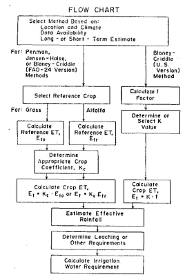
A flow chart is presented in Fig. 6.1 outlining the sequential steps for estimating irrigation water requirements from climatic data. These steps are intended to apply to the information presented in this chapter. A similar se-quence would be valid for any other source of data.

Important considerations. Observed ET rates for a given crop and growth stage depend on climatic conditions. Water use rates observed at one location may not apply elsewhere. For example, the peak monthly ET rate at Brawlcy, California, an arid inland location is 2.5 times that at a coastal location at Lompoc, California (Jensen, 1974). In a California coastal valley the summertime ET from alfalfa 37 km (23 mi) inland was found to he more than L5 times that 29 km (13 mi) nearer the ocean (Nixon ct al., 19631. Con-versely, measured or calculated ET values might properly be transferred con-siderable distance where rather uniform conditions of climate and cropping practices exist on relatively flat terrain.

Calculate Irrigation Water Requirement Select Method Based on:

Location and Climate Data Availability

Long - or Short - Term Estimate

For Penman, Jensen-Noise, or Blaney- Criddle (FAO-24 Version) Methods

Select Reference Crop

Alfalfa

Calculate Reference ET,

E tr

Determine Appropriate Crop

Coefficient, Kc

Calculate Crop ET. E t • Kc E t o or E t • K c E t r

•

Blaney -Criddle (U. S.

Version) Method

Calculate f Factor

Determine or Select K

Value

Calculate Crop ET, E t • K • f

Estimate Effective Rainfall For: Grass

Calculate Reference ET,

E to

Determine Leaching or Other Requirements FLOW CHART

FIG. 6.1 TypIca flow chart for estimation of irrigation water re-quirements from climatic data.

Factors contributing to water requirements. ET is the principal factor in determining irrigation water requirements, but losses in storage, conveyance and applying water, the inability to apply water uniformly, and the need for soil leaching are additional factors. The planning and operation of irrigation systems must take all these factors into consideration in determining water requirements. _{Other possible requirements and uses for water not directly} re-quired for ET arc discussed under other beneficial uses in Section 6.6, and in Chapters 2, 14 and 18.

6.4 SELECTED METHODS OF ESTIMATING REFERENCE CROP ET Many _{methods of estimating ET have been proposed. The methods may} be broadly classified as those based on combination theory, humidity data,

radiation data, temperature data, and miscellaneous methods which usually involve multiple correlations of ET and various climatic data. The design engineer or hydrologist unfamiliar with methods is often faced with a bewildering choice. Several publications discuss the choice of methods kr various climatic conditions and for various amounts of input climatic data. Among these are a United Nations Food and Agriculture Organization publication, (FAO-ID 24), (Doorenbos and Pruitt, 1977) and a report of the ASCE Irrigation Water Requirements Committee (ASCE-CU Report) (Jensen, 1974).

Recent research by micrometerologists and soil scientists has separated ET calculations into evaporation from the soil and transpiration components (Ritchie, 1974). The transpiration rate has been successfully related to the leaf area index of the plants, the soil moisture status and potential transpira-tion rate. These have not been used in engineering calculatranspira-tions and have not been refined for a wide range of conditions and therefore, are not presented here. The reader should be aware that these methods may come into wider use in the future.

This chapter presents detailed step-by-step instructions for three of the most commonly used methods of estimating ET for a reference crop l.lus the use of evaporation from pans as an index of E,,. The reader is referred to other sources for other methods such as Doorenbos and Pruitt (1977) and Jensen (1974).

6.4.1 Basis for Reference ET

Reference crop ET selected must be compatible with the crop coeffi-cients (IC) that are to be used. For example, IC used to calculate ET based on alfalfa reference ET must not be used with an E„ intended to simulate grass. The reverse is equally illogical. Engineers also must be certain that the method of estimating E,, is, related to the same base as was used for the development of the crop curves that they are using. The Penman and Jensen-liaise methods cited in this chapter both estimate E„ based on alfalfa because these are compatible with recently developed crop coefficients for the Western United States (Wright, 1979). The Blaney-Criddle and pan evapora-tion methods described in this secevapora-tion are recent FAO modificaevapora-tions which estimate grass based reference El .

Doorenbos and Pruitt (1977) also present modifications of the Penman method and radiation methods in the FAO publication, which as the first step requires estimates of grass based reference ET. The FAO procedures also require using grass based crop coefficients. The FAO procedures cover a very broad range of wind, sunshine, and humidity conditions because they are based on a world-wide data set. The Penman method presented in this chapter is particularly suited to irrigated areas in the Western United States because of recently developed alfalfa based crop coefficients (Wright, 1979).

6.4.2 Penman Method

16.1 [6.6]

1. 0.386 P

7-

_{u, _ U, (}

where a (m) is the elevation of the wind measurement and U2 is the estimat wind travel at 2 m.

Various procedures have been used to calculate the saturation vdp pressure deficit term (e. - ed) of equation [6.4] and sometimes the meths used has not been cIeárly identified. Two possible methods are describ' here. Method 1 uses the saturation vapor pressure at mean air temperatti

as ew and the saturation vapor pressure at the mean daily dew poi temperature as ed. This method is described in more detail by Doorenbos al Pruitt. Method 2 is more applicable in arid areas and high elevations wile large diurnal temperature changes occur:

Ca 2 = -1 (e

a max + ea min) 6.1

TABLE 6.2. SELECTED VALUES OF a w AND h„, FOR VARIOUS WIND FUNCTIONS FOR THE PENMAN METHOD

Mvtilod of

c,dru-Reference lating

No. Author(s) Crop _{a ,, b w} (e a - e d )

1 Penman (1963) Cupped

graft 1.0 0.00021 1

2 Wright and Jensen

(1972) Alfalfa 0.75 0.0115 2

3 Doorenbos and Pruitt

(1977) Grass 1,0 0.01 1

4 Wright (1981) Alfalfa (varies with time) 2 ..•

from the theoretical basis of the methods. Estimates.obtained with a com-bination equation arc reliable for periods of from 1 day to 1 month. With modifications, reliable hourly estimates arc possible.

The Penman equation, modified for estimating alfalfa based reference ET in cal/cmz•d is :

Etz.= (Rn + G) + 7+ 7 15.36 W1 (ea - ed) [6.4]

where E„ = reference crop ET in eal/cmz•d; A is the slope of the vapor pressure-temperature curve in mb/°C; y is the psychrometer constant in inb/uC; R. is net radiation in cal/cmz•d; G is soil heat flux to the surface in

cal/cm2_{•d; W, is the wind function(dimensionless); (c. - ed) is the mean} daily vapor pressure deficit in nib; and 15.36 is a constant of proportionality in cal/cmz_{-cl•mb. An expression adapted from Bosen (1960) can be used to} approximate A:

A = 2.00(0.00738 T + 0.8072)7 0.00116 [6.5]

where T is mean daily temperature (DC). An expression by Brunt (1952) can be used to find y:

TABLE 6.1. VARIATION OF A!(.5 + ') WITH

ELEVATION AND TEMPERATURE•

m

°C 0 500 1000 1500 2000 2500

0.0 0.401 0.414 0.428 0.443 0.458 0.475 5.0 0.477 0.491 0.505 0.520 0.538 0.552 10.0 0.551 0.564 0.578 0.593 0.608 0.624 15.0 0.620 0.632 0.645 0.650 0.673 0.688 20.0 0.681 0.693 0.705 0.717 0.730 0.743 25.0 0.735 0.745 0.756 0.767 0.778 0.790 30.0 0.781 0.790 0.799 0.809 0.818 0.828 35.0 0.820 0.828 0.835 0.844 0.852 0.860 40.0 0.852 0.858 0.867 0.872 0.879 0.886 45.0 0.878 0.884 0.889 0.895 0.901 0.907 50.0 0.900 0.904 0.909 0.914 0.919 0.92-1

• 7 q

= 1 - , based on the U.S. standard

A+7 A + 'y

atmosphere.

developing the wind functions for the Penman equation. Wind data collect at another elevation can be extrapolated to the 2-m elevation by the follosriii expression which approximates a logrithmic velocity profile and is based an aerodynamically "rough" crop surface such as alfalfa:

where P is average station barometric pressure (nib) and L is the latent heat of vaporization (cal/g). P is usually assumed to be a constant for a given ion-tic,: and may be calculated using a straight line approximation of the U.S. standard atmosphere;

P = 1013 - 0.1055 E _16.7]

where E is sea level elevation (meters). L may be calculated as follows (Brunt, 1952):

L = 595- 0.51 T _[6.8]

where T is °C. The variations of A/(A y) with elevation and temperature are given in Table 6.1.

The W, term is usually determined by regression techniques where W,

has the form:

Wf = _16.9]

Rb = [a Rs

Rso

where e, max is the saturation vapor pressure at maximum daily air temperature, e, min is the saturation vapor pressure at minimum daily air temperature, and the saturation vapor pressure at the mean daily dew point temperature is used for e„. Procedures for calculating the mean daily dew point temperature or mean daily vapor pressure are sometimes not clear or consistent. Future studies and publications are expected to establish a stan-dard procedure for this.

It is extremely important to make certain that the crop coefficients to be used are based on the same W, that was used to estimate reference crop ET. For example, use the Wf _{by Wright and Jensen (1972) or Wright (1981) for}

crop coefficients presented jn Subsection 6.5.3. If the grass based E,, as defined by Doorenbos and Pruitt (1977) is used, use K, values from Subsec-tion 6.5.4 or the crop coefficient procedures presented in FAO-/D 24. They emphasize that the wind function used must also be compatible with the method used to calculate the vapor pressure deficit term (e, e„) and the crop coefficients used must have been developed using the same procedure for caIculAting (e. — e,) and the wind function Wp

The absence of humidity data is often cited as a reason for not using combination equations in engineering calculations of ET. There are alter-natives for estimating average daily dew point temperature. For example, Pochop et al. (1973) presented empirical relationships between average daily dew point temperature and daily minimum temperature for Wyoming. Saturation vapor pressure (mb) for any temperature T (°C) may be determin-ed from the following approximation of Rosen (1960):

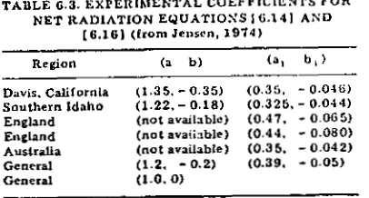
TABLE 6.3. EXPERIMENTAL COEFFICIENTS FOR NET RADIATION EQUATIONS t 6.141 AND

(6.161 (horn Jensen, 1974)

Region (a b) (a l 6 1 )

Davis. California (1.35, - 0.35) (0.35. - 0.046) Southern Idaho (1.22. - 0.18) (0.325, - 0.044) England (not available) (0.47, - 0.065) England (not available) (0.44. - 0.080) Australia (not available) (0.35. - 0.042) General (1.2, - 0.2) (0.39. - 0.05) General (1.0. 0)

shown in Table 6.3. FL, is net outgoing long wave radiation on a clear day

and may be estimated as follows:

Rbo e 11.71 X 10-8 16.151

= (al + b1 %/ad) 11.71 X 10-8 Titi [6.16]

where ed has previously been defined in this chapter, T, is average daily air

temperature in °K and some values for a, and b, can be found in Table 6.3. If humidity data are not available, the following expression developed by

Idso and Jackson (1969) may be used to calculate r:

e — 0.02 + 0.261 exp[-7.77 X 10-4 (273 - 11)2_] 16.171

es 33.8639 [(0.00738 T+ 0.8072)8 - 0.00001911.8 T+ 481

+0.001316] _[6.12] where T„ is in °K._{R„ can also be calculated from the following simplified procedure:}

Net radiation (R„) in IangIeys per day (ly/d) can he calculated from solar radiation data. A langley is a cal/cm2. The signs of IL and G (equation 16.4]) assume that heat movement toward the soil surface is positive. In practice, G is often assumed to be zero for daily E„ calculations. To estimate R„:

R.„ = (1 -t)R5-I b _[6.13]

where a is reflected short wave radiation, called albedo, expressed as a decimal. Albedo is often taken to be 0.23 for commercial irrigated crops. Merva (1975) presented an extensive table of a values. However, albedo is known to change with sun angle and can be estimated with an equation such as equation 16.361 for alfalfa at Kimberly, Idaho (Wright, 1981), if sufficient data are available. 12, is incoming short wave solar radiation. 12,, is net outgo-ing long wave radiation and may be estimated as follows:

+ Rbo _16.14]

where R,„ is clear day solar radiation, i.e. the solar radiation expected on a day without clouds. A clear day radiation curve can be plotted from several years of solar radiation data with the upper envelope forming the clear day radiation curves. Some experimentally determined cnetiti-ientc a ;Ind h ern

= a 3 R, + la3 16.181

An extensive table of values of as and 1)3 was presented in the ASCE-CU

Report (Jensen, 1974).

Penman's original method (Penman, 1948) called for an initial estimate of evaporation from a hypothetical open water surface and then its conver-sion to potential ET by an empirical coefficient which varied with the season. Doorenbos and Pruitt (1977) developed a somewhat similar approach, but their corrections are related to maximum humidity, the ratio of daytime to night-time winds and wind velocity; their procedures are recommended for E,,, estimates of periods from 10 days to 1 month.

6.4.3 Jensen-Ifaise Method

The Jensen-Haise method (Jensen and Hake, 1963) is another procedure for estimating ET from climatic data. Though the method is often classified as a solar radiation method, air temperature is also used and the coefficients are based on other input parameters such as elevation and long term mean temperature. The method produces an estimate of an alfalfa E,, as defined by Jensen et al., (1970). Doorenbos and Pruitt (1977) also presented a solar radiation method for estimating E.. for grass. The reader is again cautioned that both the method of estimating E,, and the crop coefficients must be

Daytime wind may be estimated from daily wind by using the ratio day to night winds.

[6.221 percent sunshine.

U day/U night ratio 1.0 1.5 2.0 3.0 3.5 4.0 Correction for U day 1.0 1.5 1.33 1.5 1.56 1.6 [6.23]

The Jensen-Raise method is the result of a review of about 3000 measurements of ET that were made in the Western United States over about a 35 year period. The method presented in this chapter is known as the "Modified Jensen-Haise" method. The ASCE 1rrigaton Water Requirements Committee recommended that estimates using the Jensen-Haile method be made for periods of 5 days to a month.

The Jensen-Haise method is as follows:

E tr =- C T - Tx )its 16.191

where E,, has the same units as R, and is compatible with alfalfa based crop coefficients.

1 CT - CI +7.3 CH

c 50 mb

H e 2 - e t

[6.20]

[6.21j

where c2 is the saturation vapor pressure of water in nib at the mean monthly maximum air temperature of the warmest month in the year (long term climatic data), and c, is the saturation vapor pressure of water in nib at the mean monthly minimum air temperature of the warmest month in the year.

where E = the site elevation in m. Tx = - 2.5 - 0.14(e2 - el)

-Solar radiation may be measured or estimated.

6.4.4 Blaney-Criddle Method

The Blaney-Criddle method was first proposed in 1945 by H. F. Blaney and W. D. Criddle (Blaney' and Criddle, 1945) and was based on Western USA field measurements of ET. The method has been revised many times and there are so many variations that when the method is used the authors must he very careful and complete in their identification of the exact varia-tion used. Perhaps the best known variavaria-tion in the United States is that found in Technical Release No. 21 of the USDA Soil Conservation Service (USDA SCS, 1970). The method has been used on a world-wide basis but local calibration has been considered highly desirable.

The Blaney-Criddle method is based on the principle that ET is propor-tional to the product of daylength percentage and mean air temperature. The monthly constant of proportionality has been called the crop growth stage coefficient. This coefficient is not the same as the crop coefficient defined by equation [6.1] and [6.2]. Estimating ET by the early versions of the Blaney-Criddle method is a single stage process which does not involve the

in-termediate step of estimating reference crop ET. Estimates have been con-sidered to be valid for monthly periods (Jensen, 1974). The one stage Blaney-Criddle method is widely used in the intermountain region of the United States, with local calibration, for water right deliberations (Kruse and Haise•

1974; Burn/an, 1979).

A recent major revision of the Blaney•Criddle method was published b FAO (Doorenbos and Pruitt, 1977). The FAO Blaney-Criddle method fu produces a reference crop ET estimate for grass (see Subsection 6.2.2). 'Ill FAO modifications were based on data from 20 locations representing a vel wide range of climatic conditions.

The FAO variation uses air temperature measurements for the site question. The need for local calibration is minimized by the classification c climate at a site based on daytime wind, humidity and sunshine. For then classifications general estimates of wind, humidity or sunshine from source such as a climatic atlas or more exact data may be used.

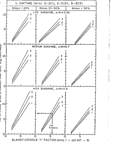
The FAO variation of the Blaney-Criddle method is as follows:

E ta = a 4 + b 4 f [6.2

= p(0.46 + 8) [6 2

where E,,, is in mm/d, p is the percentage of daytime hours of a day compare to the entire year (see Table 6.4), and T is the average monthly ai temperatures, °C.

The numbers a, and b, represent the intercept and slope of a straigh line relationship between E„„ and f. E,„ may be determined directly from using Fig. 6.2 and classifications of daytime wind, minimum humidity all

TABLE 6.4. MEAN DAILY PERCENTAGE (p) OF ANNUAL. DAYTIME HOURS FOR DIFFERENT LATITUDES 2 E

C1 =38-305 305 1 Latitude North South • Jan July Feb Aug Mar Sept Apr Oct May Nov June Dec July Jan Aug Feb

Sept Oct Mar Apr

S•I)t N1,sy (")c 0.1 0.1 0.1 , 0.1 0.1 0.1. 0.1' 0.2 0.21 0.21 0.2: 0.2: 0.24 0.2:" 0.2.! 0.2 ,r• 0.27 0.2•: GO deg 58 56 64 52 50 48 46 44 42 40 35 30 25 20 15 10 0 0.15 0.16 0.17 0.18 0.19 0.19 0.20 0.20 0.21 0.21 0.22 0.23 0.24 0.24 0.25 0.26 0.26 0.27 0.27 0.20 0.21 0.21 0.22 0.22 0.23 0.23 0.23 0.24 0.24 0.24 0.25 0.25 0.26 0.26 0.27 0.27 0.27 0.27 0.26 0.26 0.26 0.26 0.27 0.27 0.27 0.27 0.27 0.27 0.27 0.27 0.27 0.27 0.27 0.27 0.27 0.27. 0.27 0.32 0.32 0.32 0.31 0.31 0.31 0.31 0.30 0.30 0.30 0.30 0.29 0.29 0.29 0.28 0.28 0.28 0.28 0.27 0.38 0.37 0.36 0.36 0.35 0.34 0_34 0.34 0.33 0.33 0.32 0.31 0.31 0.30 0.29 0.29 0.28 0.28 0.27 0.41 0.40 0.39 0-38 0_37 0_36 0.30 0.35 0.35 0.34 0.34 0.32 0.32 0.31 0.30 0.29 0.29 0.28 0.27 0.40 0.39 0.38 0.37 0.36 0.35 0.35 0.34 0.34 0.33 0.33 0.32 0.31 0.31 0.30 0.29 0.29 0.28 0.27 0.34 0.34 0.33 0.33 0.33 0.32 0.32 0.32 0.31 0.31 0.31 0.30 0.30 0.29 0.29 0-28 0.28 0.28 0.27

0_28 0.22 0_28 0.23 0.28 0_23 0.28 0_23 0.28 0.2-1 0.28 0.21 0.28 0.2.1 0_28 0.24 0.28 0.25 0.28 0.25 0.28 0.25 0.28 0.25 0_28 0.26 0_28 0.26 0.28 0.2G 0.28 0.27 0.28 0.27 0.28 0.27 0.27 - 0.27

r

_

Pll I

3

---2

IP

LOW

....

..-SUNSHINE, n/N 0.45

_ 3

___

-

,-—

—

1 1 P a, 1 1 1 I

-..

, _ —

—

.

2

1 t I 1 3

2

1 1

MEDIUM

'•

SUNSHINE, n/Nr40.7

— 3

- 2

_

-k ill L. 11 1 1

—

_

-,

I

3

2

.. _

•

I 1 1 1 1 1 1 1

3 -2

-1.

-_

-.,

k

HIGH SUNSHINE, n/N0.9

2

I

1

July,

Kimberly ;

1 I I I 1 t/ 1 1 !I i 11 2

5 q 5 0 5

BLANEY•CFtIDDLE "f" FACTOR (mm), f p(0.46T * 8)

FIG. 6.2 Prediction of reference ET for grass (E..) from Iliane)-Critidle (factor for different con-ditions of minimum relative humidity, sunshine duration and day-time wind (from Doorenbos and Pruitt, 19771.

The minimum relative humidity is the ratio of saturation vapor pressure at average dew point temperature to that at maximum air temperature.

Doorenbos and Pruitt (1977) recommend that individual calculations be made for each month of record and that values of E,. may need to be

increas-rrj hifrtIrr fq1.1111intic nr• 1,,t;117,4/.

-from 10 days to one month. For computerized applications. Doorenbos and Pruitt (1977) recommend interpolation of the slope of the line from an exten-sive table and the intercept from humidity and sunshine inputs.

6.4.5 Pan Evaporation Method

Evaporation pans are an integral part of most agricultural weathcr sta-tions. if the stations are visited weekly or more often and the operator is diligent, excellent data may be collected. Reference crop Er may be estimated by the following relationship.

E = K E_{to p p}

where E,. = pan evaporation in any desired units, for example mm/d, K, dimensionless pan coefficient, and E,„ = reference crop ET (grass) in the same units as E.

Since E,o represents grass ET (see Subsection 6.2.2) it is therefore man-datory that crop coefficients (K.) used to convert E,, to ET for a specific crop and time be taken from Subsection 6.5.4 or from FAO-ID 24. The informa-tion in this Subsecinforma-tion, while useful in interpreting data from existing pans, is intended more as guidelines for locating evaporation pans specifically in-tended for estimating ET.

Data from evaporation pans have been correlated with El for many years because pan evaporation integrates many of the factors involved in ET; these include wind, radiation, humidity and air temperature. The evapora-tion pan however is inanimate and does not reflect heat storage and transfer characteristics of a crop. For literature review the reader is referred to Doorenbos and Pruitt (1977) and Jensen (1974).

Types of pans. Discussion in this Subsection is limited to the U.S. Class

A Pan. This pan is 121 cm in diameter and 25.5 cm deep. The pan is usually

constructed of galvanized steel or Monet metal. The pan is placed on a wooden platform and leveled. The bottom of the pan is usually about 15 cm above ground level. The water level is maintained within a range of from 5 to 7.5 cm below the rim by careful water additions, or by a float system and a supply tank. Changes in water level are measured by a vernier hook gage placed in a stilling well. Many other types of evaporation pans have been used; these include different sizes, depths, screens and many arc buried below the ground surface (also see Subsection 165,3). Dooren hos and Pruitt (1977) present a table of factors plus narrative discussion relating various sizes of pans to the Colorado Sunken Pan. 1-lounam (1973) also discusses various sizes, types of pans, and their relative performance.

Selection of K,, values. The pan coefficient varies with pan exposure,

wind velocity, humidity, and distance of homogeneous material to the

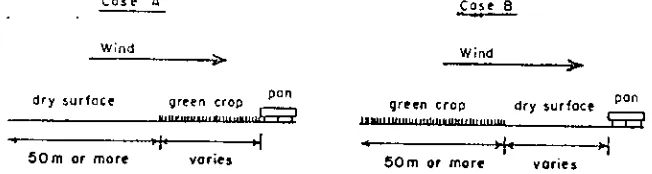
wind-ward side (fetch). Values of K„ for periods of 10 days to a month may be selected from Table 6.5. Additional factors arc discussed later. Table 0.5 is self explanatory except Cases A and B need further elaboration. Case A defines the condition where air moves across at least 50 in of dry surface and then across from I to 1000 m of a green crop. The situation is reversed in

Case B; see the sketch below for a visual interpretation. Doorenbos and

Pruitt (1977) also present a similar table for use with the Colorado sunken pan.

5

E E 10

0

2

c

Er)

0

a.

IA 10

Cr. tL tit 5 tx

0

Case a

Wind

pan green crop dry surface

Case 0

Wind

green crap dry surface pan

50m or more varies _{50m or more} sit _varies

Additional factors. Many additional factors can modify the pan coeffi-cients found in Table 6.5. For example E,, may be increased by 10 percent if the pan is painted black. If Pans are placed in a small enclosure surrounded by tall crops, 1C, may need to be increased by up to 30 percent for dry windy climates, and only from 5 to 10 percent for calm humid climates. The coeffi-cients presented in Table 6.5 assume no screen is present, that no crops taller than I m are within 50 m and that the area within 10 m of the pan is covered by a frequently mowed green grass cover or by bare soils. Doorenbos and Pruitt (1977), Jensen (1974), and Hounam (1973) discuss additional factors that influence pan evaporation.

Location and operation of pans. A weather station which includes an evaporation pan should be located so that its surrounding conditions are easy to classify and maintain in as constant a condition as possible. The

tempta-TABLE 6.5. PAN COEFFICIENT IC„ FOR CLASS A PAN FOR DIFFERENT GROUND COVElt AND LEVELS OF

MEAN RELATIVE HUMIDITY AND 24 ft WIND (For use In equation I6.263 to estimate E tc).

Case A _{Case Bt}

Class A Pan Pan surrounded by short green crop Pan surrounded by dry-fallow land

low medium high low

RH mean % 40 _{< 40 40-70 > 70 < 40}

Upwind Unwind

distance of _{distance of}

Wind green eras> dry fallow

km /day

Light o 0.55

< 175 10 0.65

100 0.7 1 000 0.75

Moderate _{o 0.5}

175-425 10 0.6

100 0.65 1 000 0.7

Strong 0 0.45

425-700 10 0.55

100 0.6

1 000 0.65

Very strong 0 0.4

> 700 10 0.45

100 0.5 1 000 0.55

'(For extensive areas of bare-tallow soils and not agricultural development, reduce Roan

values by 20 percent under hot windy conditions, by 5 to 10 percent for moderate wind, temperature and humidity conditions.

Total wind movement km /d.

tion to place the station in an unused or otherwise convenient but unrepresentative location should be resisted. The pan's location should be dictated by the intended purposes. With proper location and care in use, reference crop ET estimates to ± 10 percent accuracy should be possible.

6.4.6 Local Calibration

All methods of estimating ET from climatic data involve empirical rela-tionships to some extent. Even the combination equation, the Penman method for example, utilizes an empirical wind function. The empirical rela-tionships account for many local conditions. The ASCE irrigation Water Re-quirements Committee stated that ". .. no single existing method using meteorological data is universally adequate for all climatic regimes, especial-ly for tropical areas and for high elevations, without some local or regional calibration" (Jensen, 1974). If the crop economic importance is high, local calibration is needed to at least give confidence to irrigation wa.er require-t ment estimates. Doorenbos and Pruitt (1977) present a detailed description of a world wide calibration of the Blaney-Criddle, radiation, and Penman methods. The principles can be applied to a local or regional calibration.

Calibration involves the simultaneous collection of field E, data and the corresponding climatic data. The time interval for ET estimates has an in-fluence on the methods that are used for field measurements. Preferably. if the method is to be used for short period estimates, comparable data should be used in calibration.

Blaney-Criddle method. The Blaney-Criddle method is suited for monthly estimates of ET, (Jensen, 1974). Therefore, field measurements of El' can be made using careful soil moisture measurements, water table lysimeters, drainage lysimeters, weighing lysimeters or inflow-outflow techni-ques. Only air temperature and rainfall data are needed to complete the calibration by determining the appropriate monthly crop coefficient.

Jensen-Haise method. The Jensen-Hake method is recommended for 5-day to 1-month periods (Jensen, 1974). Drainage lysimeters are only suitable for 10-day or longer periods (Doorenbos and Pruitt, 1977), and can be eliminated if short period calibration is desired. Er measured by soil moisture change can also be eliminated for short period calibrations. Therefore, if 5-day periods are desired, weighing lysimeters or Bowen ratio techniques should be used to collect the necessary field ET data for local calibration. For monthly calibration, ET may be determined by properly per-formed measurements of soil moisture depletion, inflow-outflow, lysimeters or other techniques. Climatic data should include solar radiation, air temperature and rainfall data on at least a daily basis.

Local calibration of both Cr and T. can be obtained by regression of measured E„ /R„ against mean air temperature if data are available from about 5 to 30 °C, or higher. If only a few data points are available over a nar-row temperature range, then these data should be used to adjust the T. value, but not the Cr value.

Penman method. The Penman method can provide accurate estimates of ET for periods of 1 month to 1 hour depending on the method of calibra-tion. For short periods only weighing lysimeters can provide the necessary E. data. Climatic data must include, solar radiation, net radiation if possible, wind movement, air temperature, vapor pressure and precipitation all col-lected on intervals suitable for the desired prediction periods. Usually local 0.65 0.75

0.75 0.85 0.8 0.85' 0.85 0.85 0.6 0.65 0.7 0.75 0.75 0.8 0.8 0.8 0.5 0.60 0.6 0.65 0.65 0.7 0.7 0.75 0.45 0.5 0.55 0.6 0.6 0.65 0.6 0.65

0 10 100

0.7 0.6 0.55 1 000 0.5

0 0.65 10 0.55 100 0.5 1 000 0_45

0 0.6

10 0.5 100 0.45 1. 000 0.4

0 0.5

10 0.45 100 0.4 1 000 0.35

medium high 40-70 > 70

0.8 0.85

0.7 0.8

0.65 0.75

0.6 0.7

0.75 0.8 0.65* 0.7

0.6 0.65

0.65 0.6 0.65 0.7 0.55 0.65 0.45 0,G 0.45 0.55

0.6 0.65

0.5 0.55

0.45 0.5

GENERALIZED CROP CURVE

₁

Cornr.:ste Ir I, Kilotons

Emergence Rapid Growth Effective Full Maturation Cover

FIG. 6.3 Generalized basal ET crop coefficient curve (I).'„) with adjust-ment for increased evaporation due to surface soil wetness tiC,t to deter-mine the over-all crop coefficient (K.l•

calibrationis accomplished by calibrating the transfer coefficient identifica-tion of the variables.

= 5.36 W1 (e a - c (l) 16.271

Whenever local calibration is made, consistency between any reference crop used, crop coefficients, and calculation method used to obtain terms as e,,) must be followed. If consistency is not followed ET estimates will be illogical and may not represent the crop grown. For daily calibration of the Penman method see Wright (1981) and Subsection 6.5.3.

6.5 ESTIMATING ET FOR CROPS

Estimating ET for a specific crop can be a very complex matter depen-ding on the degree of refinement desired. To obtain the most accurate estimates, all of the major contributing crop and environmental conditions need to be taken into account. These involve climate, soil moisture, the type of crop, stage of growth and the extent to which the plants cover the soil. This section is intended to provide the means for the practicing engineer or irriga-tion scientist to integrate these inter-related factors into the best possible ET estimates. The procedures primarily involve the use of an estimated reference ET and experimentally developed ET crop coefficients. Such procedures are now extensively used in irrigation scheduling methods and in estimating crop water requirements and have been described in detail in previous publica-tions. For purposes of this section, the most salient principles and informa-tion are provided. Those desiring more informainforma-tion should consult the listed references.

The common Blaney-Criddle method does not use ET crop coefficients. Rather, the estimations of crop ET are made in one step. The method was revised by Doorenbos and Pruitt (1977) to provide an estimate of E r, for grass so that appropriate crop coefficients could be used to estimate ET for a specific crop. Such procedures produce estimates with accuracies suitable for

10-day to monthly periods.

Detailed and specific procedures and guidelines were summarized by Doorenbos and Pruitt (1977) for predicting crop water requirements for a wide range of crops and conditions and availability of associated informa-tion. They outlined a three-stage procedure involving (a) a reference crop ET, (b) a crop coefficient, and (c) the effects of local conditions and agricultural practices. They chose ET for 8- to 15-cm tall, green, well-watered grass as the reference ET and selected or adapted crop coefficients accordingly. Four methods of estimating this reference ET were presented, namely: (a) Blaney-Criddle, (b) radiation, (c) Penman, and (d) pan evapora-tion. In this section, we present crop coefficients for E. based on alfalfa, as defined by Jensen et al. (1970) suitable for daily estimates of ET when E,, is determined by the Penman method described in this chapter. These alfalfa based coefficients are also suitable for the Jensen-Raise method as presented in Subsection 6.4.3. We also present a limited set of crop coefficients based on grass E,, which are intended for use with the FAO Blaney-Criddie and pan evaporation methods described in Subsections 6.4.4 and 6.4.5.

6.5.1 Crop Coefficients ,

Experimentally developed crop coefficients reflect the physiology of the crop, the degree of crop cover, and the reference ET. In applying the

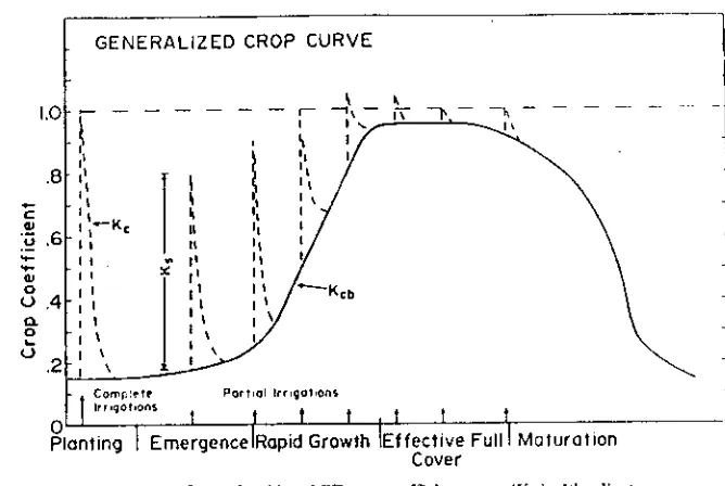
coefti-eients, it is important to know how they were derived since they are empirical ratios of crop ET to the reference ET, as shown in equation [6.11. The com-bined crop coefficient includes evaporation from both the soil and plant sur-faces. The contribution of soil evaporation is strongly dependent upon the surface soil wetness and exposure. Transpiration is primarily dependent upon the amount and nature of plant leaf area, and the availability of water within the root-zone. Crop coefficients can be adjusted for soil moisture availability and surface evaporation. The distribution of crop coefficients with time is known as a crop curve. See Fig. 6.3 and 18.1 for examples of crop curves. Other time-related crop parameters may also be used as a base.

In the experimental determination of crop coefficients, ideally both crop ET and reference ET are measured concurrently. The crop coefficient is then calculated as the dimensionless ratio of the two measurements. Well sited, sensitive weighing lysimeters provide ideal daily measurements and problems with soil-water drainage are avoided. Care must be taken to insure that border effects are minimized, that fetch is adequate, and that crop and soil moisture conditions are similar in the lysimeter and the field.

6.5.2 Reference ET

Daily rates can be accurately measured with sensitive weighing lysinmers. However, it is not possible to maintain the crop surface in a con-dition to provide near maximum ET because of cutting periods, lodging of plants by _{wind or rain, and the effects of late and early seasonal frosts.} Con-sequently, daily alfalfa ET, energy. balance, and meteorological data can be used to develop and calibrate procedures for computing reference El'. The computed reference then can be used to extend the measured values for periods or locations where measured values are _{not available.}

6.5.3 Alfalfa Related Crop Coefficients

An overall daily crop coefficient can be determined from daily measured reference and crop ET by:

K = _C -_pE --tr

in which K, = the dimensionless crop coefficient for the particular crop at the existing growth stage and surface soil moisture condition. When estimating crop ET front the reference ET, K, is estimated from crop curves for the day or period involved and informatio'n on soil moisture conditions by:

K c = K cb K a + Ks _[6.29]

in which K, = daily crop coefficient, K„ = daily basal ET crop coefficient, K, = a coefficient dependent upon available soil moisture, and K, = a coef-ficient _{to allow for increased evaporation from the soil surface occurring after} rain or irrigation. These procedures are described in greater detail by Jensen (1974), and Jensen et al. (1971). The generalized basal crop coefficient, was defined by Wright (1979) to represent conditions when the soil surface was dry so that evaporation from the soil was minimal but soil-water availability did not limit plant growth or transpiration, i.e. K,

₌

= I and K. 0. He determined daily values of K„ by manually fitting a basal crop curve to overall crop curves obtained with equation [6.28]. This specific designation also distinguished the K,5 values obtained with lysimeter ET data from mean crop coefficients previously developed from soil-water-balance data.

When available water within the root zone limits growth and ET, K. of equation [6.29] will be less than 1.0 and can be approximated by relation-ships similar to:

K a = [ln(Aw + i)]/[111(101)] _[6.30]

in which AW = the percentage _{of available water (100 when the soil is at field} capacity), and K. = 1 when A., 100, and K. goes to zero as A., goes to 0. This algorithm was developed from published ET-soil water data (Jensen et al., 1971). Other relationships for K. were reviewed by Howell (1979).

Increased soil evaporation due _{to rainfall or irrigation, can be estimated} by:

Ks = (K1 _{- K ci )exp (-At), K i >Kci [6.311}

in which t the number of days after the rain or irrigation; A the combin-ed effects of soil characteristics, evaporative demand, etc; and K„ the value of K,, at the time the rain or irrigation occurred. This algorithm will also vary for various soils and locations. At Kimberly, Idaho K, was approx-imated by (0.9 - K,)0.8; (0.9 - K,)0.5; and (0.9 - K,)0.3; for the first. se-cond, and third days after a rain or irrigation, respectively (Jensen et al., 1971). When K. exceeds 0.9 no adjustment is needed for rain or irrigation. A diagramatic representation of the expected changes in the crop coefficient as affected by stage of growth and wet surface soil, is presented in Fig. 6.3.

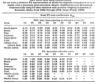
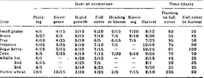
A summary of basal crop coefficients for several crops is presented in Table 6.6 for arid areas. These were derived for use with estimated El" for a reference crop of actively growing, well watered alfalfa at least 20-cm tall. Dates typical of Kimberly, Idaho for planting, emergence, effective cover, and harvest for the various crops are presented in Table 6.7.

Values of K, are listed on a normalized time scale, instead of actual dates, with time from planting until full cover on a percentage basis,

KT,

development. Alfalfa cuttings are listed individually because of major dif-ferences in climate for each of the growth periods.

The alfalfa related crop coefficients described in this section were com-puted using the Penman method discussed in Subsection 6.4.2 with some modifications. Suitable procedures have been described in many

publica-TABLE 6.6. DAILY BASAL ET cam,COEFFICIENTS (Rd) ) FOR DRY SURFACE SOIL CONDITIONS

for use with a reference ET representative of alfalfa for irrigated crops grown i n an arid region with a temperate inter-mountain climate. Coefficients were determined

experimentally using ET data obtained with sensitive weighing lysimeters at Kimberly. Idaho. from 1968 through 1978, (from Wright. 1979)

Basal ET crop coefficients. E cb

PCT, time from planting to effective cover (%)

Crop 10 20 30 40 50 60 70 80 90 100

Small grains 0.15 0.16 0.20 0.28 0.55 0.75 0.90 0.98 1.00 1.02 Beans 0.15 0.17 0.18 0.22 0.38 0.48 0.65 0.78 0.93 0.95 Peas 0.20 0.17 0.16 0.18 0.20 0.28 0.48 0.67 0.86 0.95 Pots toes 0.15 0.15 0.15 0.21 0.35 0.45 0.60 0.72 0.78 0.80 Sugar beets 0.20 0.17 0.15 0.15 0.16 0.20 0.30 0.50 0.80 1 00 Corn 0.15 0.15 0.16 0.17 0.18 0.25 0.40 0.62 0.80 0.95 Alfalfa (Ist) 0.50 0.58 0.67 0.75 0.80 0.85 0.90 0.95 0-98 1.00 (2nd Sr 3rd) 0.50 0.25 0.25 0.40 0.55 0.79 0.80 0.90 0.98 1.00 Winter wheat 0.65 0.70 0.76 0.80 0.85 0.90 0.95 0.98 1.00 1 02

DT, days after effective tuver

10 20 30 40 50 60 70 80 90 100

Small grains 1.02 1.00 0.80 0.50 0.25 0.10 0.10 Beans 0.95 0.94 0.65 0.36 0.18 0.15 0.10 Peas 0_93 0.82 0.50 0.37 0.20 0.10 0.10

Potatoes 0.80 0.80 0.75 0.74 0.73 0.72 0.70 0.50 0.25 0.20 Sugar beets 1.00 1.00 1.00 0.96 0.93 0.89 0.86 0.83 0.80 0.75 Corn 0.95 0.95 0.93 0.91 0.89 0.83 0.76 0.30 0.20 0.15 Alfalfa (142) 1.00 1.00 1.00 0.25

(3rd)* 1.00 1.00 0.52 0.30

Winter wheat 1.02 1.00 0.96 0.50 0.20 0.10 0.10

6w(r) = - 0,0122 + (5.2956E-04)D - (5.9923E-06)D2

+ (3.4002E-08)03 - (9.00872E-11)04 (8.79179E-14)D5

16.351

where D is the day of the year and the polynomial coefficients are for wind travel measured at 2 m in km/d. Respective values for 4/15, 6/15, 8/15, 10/15, and seasonal mean for a,.. are: 0.74, 1.83, 1.01, 0.55, and 1.06; and for b..: 0.0069, 0.0088, 0.0107, 0.0099, and 0.0091. These mean values com-pare with the seasonal Penman coefficients of 1.0 and 0.0062 and 0.75 and 0.0115 of Wright and Jensen (1972, 1978) (also see Table 6.2).

The net radiation term, R„, of equation [6.4] was estimated from daily solar radiation, temperature, and humidity data by equations [6.13] to [6.16] using values and functions as developed by Wright (1981) for Kimberly, Idaho. The albedo (a) was computed by:

a = 6.29 + 0.06 SIN I 30[M+(N/30) + 125]

t

where M is the number of the month and N is the number of the day. The season long regression coefficients for Kimberly, Idaho arc: a, is 0.325 and b, is -0.044 (Wright and Jensen, 1972). The coefficient a, of equation [6.16] was computed with a "normal" distribution equation:

al = 0.26 + 0.1 exp 430(M+N/30)-207)/65)21- [6.371 A constant value of b, of -0.044 was used with the variable a,. Coefficients for equation [6.14] were: for RJR,„ greater than 0.7; a 1.054 and b = 0; and for R,/ R,„ less than or equal to 0.7, a = 1.0 and b = 0.

TABLE 6.8. DAILY BASAL ET CROP COEFFICIENTS ( g ad FOR USE WITH GRASS REFERENCE ET MO

for Irrigated crops grown in an arid hiediterrancan climate. Coeff icients are for dry soil surface conditions and were determined experimentally with ET data obtained with sensitive weighing lyslmeters at Dovis. CA, 1965-1975. Days from planting to effective

full cover and from then to harvest or maturity are listed

Crop

Plant-ing

date Days topeak Kc

Time from planting to peak K c ,

10 20 30 40 50 60 70 80 90 100

Sorghum 5/17 45 0.12 0.13 0.14 0.16 0.22 0.33 0.50 0.75 Lau 1.07 Beans 6/21 43 0.10 OA 2 0.16 0.31 0.28 0.39 0.53 0.75 0 98 1.08 Tomatoes 4/29 80 0.14 0.15 0.17 0.19 0.22 0.33 0.48 0.71 1 04 1.18 BarIev 10/31 100 0.18 0.20 0_22 0.24 0.28 0.34 0.47 0.66 0.90 1.07 Corn 5/14 52 0.12 0.13 0.15 0.20 0.29 0.45 0.81 0.99 1.09 1.13 Sugar beets

(late) 6116 55 0.12 0.13

0.16 0.20 0.29 0.45 0.65 0.87 I 04 IA0 Sugar beets

(early) 3/25 _{Da y s}90 0.14 0.16 0.18 0.22 _{Days after peak E ,}0.27 0.37 0.53 0.77

1.0 1.10 Harvest to

10 20 30 40 50 60 70 80 90 100

date harvest

Sorghum 9/13 74 1.08 1.06 1.03 0.99 0.94 0.88 0.79 0.65 Bean; 9/18 46 1.12 1.12 1.10 0.71 0.15

Tomatoes 9(24 68 1.24 1.21 1.12 1.03 0.90 0.75 0.58

Barley 5/19 100 1.15 1.17 1.19 1.21 1.19 1.12 0.98 0.75 0.50 0.24 Corn 9/20 77 1.17 1.17 1.17 1.14 1.03 0_87 0.67

Sugar beets

(late) 11/18 100 1.15 1.16 1.16 1.16 1.15 1.14

1,13 1.12 1.10 1.08 Sugar beets 9420 90 1.13 1.15 1.15 1.14 1.13 1.1.1 1.08 1.05 1 01

(Carly) TAMA•. 6.7. DATE OF VARIOUS CROP GROWTH STAGES IDENTIF1A OLE

1N TUE Fi FUJI CROPS STUDIED AT KIMBERLY, IDAHO. 1068-1978 (from Wright. 1979)

Crop Plant-ing

Date of occurrence Time (clays)

Emer-genre growthRapid coverFull or bloom Heading Ripan-ing liarvest

Plan tine

to full

cover to harvestFull cover Sinall grains 4/1 411 5 5410 6120 6/15 7/20 8/15 80 55

Roans 6/22 6/5 6/15 7/15 715 8/10 8/30 55 45

Pras 4/10 4/25 5/10 6/5 6/15 715 7/25 55 50

Potatoes 4/25 5/25 6/10 7/10 7/1 10/10 75 90

Sugar beets 4/15 5/15 6110 7115 19/15 91 100

Corn 5/5 5/25 6/10 7/15 7110 9/10 9/20 79 70

Alfalfa 1st 4/I 4/20 5/15 6/15 45 35

2nd 6/15 6/25 7/5 8/1 20 35

3rd 811 8(10 8/25 9/20 25 25

1V inter wheat 10/1 10115 3/20 4125 6/5 7/15 8/10 205 60

tions, such as those of Jensen (1974), Jensen et al. (1971), Wright and Jensen (1972)j Wright and Jensen (1978), and Wright (1981). Other methods can also be adapted, but as mentioned earlier in this chapter, the combination equation seems to give the most consistent results, particularly in arid ir-rigated regions subject to considerable sensible heat advection. To adequate-ly account for advection, even the combination equation should be calibrated or verified for local conditions.

The changes necessary to permit estimating reference ET for a crop of well watered, actively growing alfalfa, at least 20-cm tall, are presented here for convenience of the reader. This follows procedures developed earlier with recent refinements by Wright (1981). Measurements or estimates of the following daily meteorological parameters are required: (1) solar radiation, (2) maximum and minimum air temperature, (3) average humidity, or at least an 0800-h dew-point temperature, and (4) wind travel.

A combination equation similar to that in Subsection 6.4.2 was used to estimate a reference ET for the development of the basal crop coefficients by:

Etr = 10 -L [6.32]

where Er, is on a water depth equivalent basis (mm/d), E, is the latent heat flux computed with the calibrated equation (cal/cm2•d), L is the latent heat of vaporization (cal/en-13), and 10 is for unit conversion (mm/cm). A wind function with time dependent coefficients was used.

= a w (t) b w (t) [6.331

where W. is the wind function and ri,,(t) and b.,(t) are variable coefficients to adapt the _{function to the location or time of year. Varying the wind function}

permits adapting Wf _{to changing conditions of the surrounding area which} influence sensible heat advection. The following empirical relationships were derived for Kimberly, Idaho.

aw(t) = 23.8 - 0.78650 + (9.7182E-03)D2 - (5.4 589E-05)03

6.6 OTHER BENEFICIAL USES

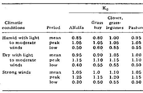
Water applied at appropriate times can sometimes make additional con-tributions to improved crop production besides the replenishment of soil moisture. While meeting the ET need of crops is the primary purpose of ir-rigation, conditions may require providing water for additional beneficial uses as discussed in Chapters 2 and 18 and briefly described in this Section. TABLE Gal. CROP COEFFICIENTS (t{,1 FOR ALFALFA,

CLOvER, GRASS-LEGUMES AND PASTURE wall mean values for between cuttings. tow values for just after

cuttings with dry soil conditions, and peak values for Just before harvest. For wet soil conditions increase low valttes

by 30% (adapted from Doorenbos and Pruitt, 1977)

K e

Clover,

Climatic Grass

grass-conditions Period Alfalfa hay legumes Pasture

Humid with light mean 0.85 0.80 1.00 0.95

to moderate peak 1.05 1.05 1.05 1.05

winds low 0.50 0.60 0.55 0.55

Dry with light mean 0.95 0.90 1.05 1.00

to moderate peak 1.15 1.10 1.15 1.10

winds low 0.40 0.55 0.55 0.50

Strong winds mean 1.05 1.0 1.10 1.05

peak 1.25 1.15 1.20 1.15

low 0.30 0.50 0.55 0.50

6.6.1 Germination of Seeds

Germination of seeds may be enhanced by irrigation at planting. and sometimes irrigation is essential for seed germination. Subsequent crop development and harvest are aided by the uniform seed germination and plant emergence. Sprinkler irrigation is especially suited to this application because the amount of water applied can be limited to the amount necessary; this is especially important where water' 'supplies are limited. Soil wetting for germination by furrow irrigation is successfully practiced in many areas, but more water is required than with sprinklers when "subbing" from furrow to ridge planted seed is involved. Furthermore, salinity tends to be concentrated in the ridge by evaporation.

6.5.5 Effect of Irrigation Method on Evapotranspiration

The method of irrigation may affect ET rates while water is being ap-plied and possibly for several days following irrigation. During irrigation, the ET rate may be highest with sprinklers because of the added evaporation op-portunity provided by the increased availability of a vapor sink and the sensi-ble energy supplied by the air layer through which the water drops travel. During windy conditions these effects are especially important due to the transport of droplets outside of the area being irrigated.

Wetting of a crop surface by irrigation (or precipitation) does not necessarily result in greater ET than otherwise. A number of studies have shown that surface evaporation replaces vegetative transpiration in equal amounts (Christiansen and Davis, 1967). In such cases ET is already at the potential rate and the site of the evaporative process is merely changed from plant stoma to the wet vegetative surface. Wetting the crop increases ET where ET has been restricted by such factors as low vegetative density and a dry soil surface, limited soil moisture available for plants, high stomata' resistance, or xerophytic plant adaptation.

At low vegetative densities evaporation from wet soil can be an impor-tant factor in contributing to ET (Ritchie, 1971). Thus, an irrigation method that does not wet the entire bare soil area can result in less ET than one that does. An advantage of drip irrigation is that it does not wet the entire soil area. However the saving of evaporation is less than the ratio of unwetted area to total bare soil area would suggest because of advective influences (also see Section 16.5).

The effect of irrigation method on ET, while of some consequence dur-ing and immediately followdur-ing irrigation, may be small on a seasonal basis. For example, Bucks et al. (1974) found that the seasonal ET for high produc-tion of cabbage in Arizona was about the same with drip, modified furrows and furrow irrigation. Lysimeter studies of grain sorghum in Texas showed no significant difierences in yield or water use efficiency (ratio of' grain yield to total crop water use) between drip and sprinkler irrigation with three ir-rigations per week (I'avelo et al., 1977).

6.6.2 Climate Modification

Climate modification may be possible using water. A large-scale effect is apparent as one drives from the desert into an irrigated area on a hot summer day and feels the effect of evaporative cooling on the atmosphere. This lower-ing of dry bulb temperature is accompanied by an increase in vapor pressure and may be accompanied by a reduction in wind speeds (Burman et al., 1975). Experiments using sprinkler or mist applications at field sites within irrigated areas have typically decreased crop temperatures 4 to 12 °C. In-creases in yield of 10 to 70 percent with such crops as peas. tomatoes, cucumbers, muskmelons and strawberries are reported, and improved quali-ty of apples and grapes have been observed (Westerman et al., 1976). However, crop response to lowered temperature stress may sometimes be less beneficial than judged from the amount of air temperature suppression. Design procedures for climate-control sprinkling and misting systems are not well developed. Misting to improve greenhouse environments is a common practice.

Evaporative cooling experiments to delay bloom of fruit trees, with at-tendant reduced danger from freeze damage, were reported by Wolfe et al. (1976). They found that with application rates of 3 L/s•ha misting systems did better than low-pressure sprinklers in keeping daytime orchard temperatures down, and thus more successfully delayed bud development until the danger of frost had passed. The mist system required only about 60 percent as much water per day of bloom delay as did the sprinklers. 6.6.3 Freeze Protection

Freeze protection can result from water applied to the soil to increase soil heat conduction and soil heat storage capacity. Significant protection may be achieved by continuous wetting of plant parts by sprinkler water dur-ing critical hours.

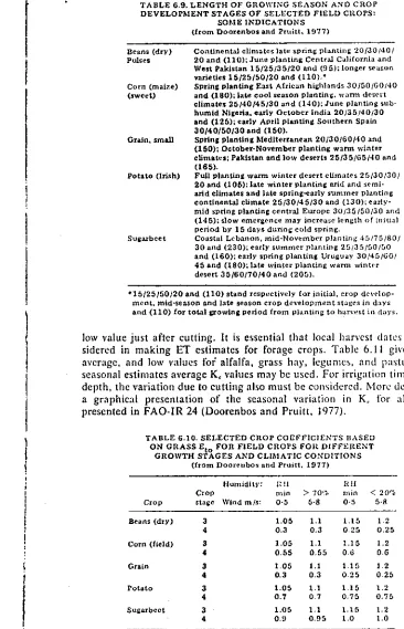
TABLE 6.9. LENGTH OF GROWING SEASON AND CROP DEVELOPMENT STAGES OF SELECTED FIELD CROPS:

SOME INDICATIONS (from Doorenbos and Pruitt, 1077)

Beans (dry) Continental climates late spring planting 20/30/401 Pulses 20 and (110); June planting Central California and

West Pakistan 15/25/35/20 and (95); longer season varieties 15/25/50/20 and (110). •

Corn (maize) Spring planting East African highlands 30/50(60140 (sweet) and (180); late cool season planting. warm desert

climates 25/40/45/30 and (1401:June planting sub-humid Nigeria, early October India 20/35/40/30 and (125); early A p ril planting Southern Spain 30/40/50/30 and (150).

Grain, small Sp ring planting Mediterranean 20/30/60/40 and (150); October-November planting warm winter climates; Pakistan and low deserts 25/35/65/40 and (185).

Potato (Irish) Full planting warm winter desert climates 25/30/301 20 and (105); Late winter planting arid and semi-arid climates and late spring-early summer planting continental climate 25/30/45/30 and (130); early-mid spring p lanting central Europe 30/35/50/30 and (145); slow emergence may increase length of initial Period by 15 days during cold spring.

Sugarbeet Coastal Lebanon, mid-November planting 45/75030/ 30 and (230); early summer planting 25135/50150 and (160); early spring planting Uruguay 30,45/60/ 45 and (180); late winter planting warm winter desert 35/60/70/40 and (205).

"15/25/50/20 and (110) stand respectively for initial, crop develop-ment, mid-season and late season crop development stages in days and (110) for total growing period from planting to harvest in days.

low value just after cutting. It is essential that local harvest dates be con-sidered in making ET estimates for forage crops. Table 6.11 gives high, average, and low values foi alfalfa, grass hay, legumes. and pasture. For seasonal estimates average K, values may be used. For irrigation timing and depth, the variation due to cutting also must be considered. More detail and a graphical presentation of the seasonal variation in K. for alfalfa is presented in FAO-1R 24 (Doorenbos and Pruitt, 1977).

TABLE 6.10. SELECTED CROP COEFFICIENTS RASED ON GRASS E to FOR FIELD CROPS FOR DIFFERENT

GROWTH STAGES AND CLIMATIC CONDITIONS (from Doorenbos and Pruitt. 1071)

Crop

Humidity : Crop

Stage Wind m/s: !1

min

0-5

7 70'7. 5-8

RH min < 0-5

20% 5-8

Beans (dry) 3 1.05 1.1 1.15 1.2

4 0.3 0.3 0.25 0.25

Corn (field) 3 1.05 1.1 3.15 1.2

4 0.55 0.55 0.6 0.6

Grain 3 1.05 1.1 1.15 1.2

4 0.3 0.3 0.25 0.25

Potato 3 1.05 1.1 1.15 1.2

4 0.7 0.7 0.75 0.75

Sugarbeet 3 1.05 1.1 1.15 1.2

4 0.95 1.0 1.0

Grass Related Crop Coefficients .

:10:rop coefficients derived for use with a reference ET for grass llliillbos" and Pruitt, 1977) are discussed in this section. A summary of 111110crop coefficients for several crops is presented in Table 6.8 similarly to

Table 6.6 except that E,„ was used as a base in their development. coefficients were obtained at Davis, California and are therefore qiii0entative of an arid. Mediterranean-type climate. Data for many

acidi-ir cropc: are presented in FAO-ID 24 (Doorenbos and Pruitt, 1977).

t

ithe

1 ;i'ztions 6.4.4 and 6.4.5 may be used to estimate E,, for use with the iii(tl,based crop coefficients. Compatible Penman and radiation methods be used. (Doorenbes and Pruitt, 1977). However, the grass-based Ilkityoefficients should not be used with the Penman and Jensen-Haise Nids as presented in Subsections 6.4.2 and 6.4.3.

and vegetable crops. The growing season may be divided into four

1

ik_i, Turves for other crops may be constructed in the following manner for a ).1" 6locat ion.

1Iii,:, Establish planting date from local information or practices in similar ili Aic zones.

y. Determine total growing season and length of crop development from local information. Guidelines to crop development stages are dlofted in Table 5.9.

l'li Initial stage: predict irrigation and/or rainfall frequency, then select lue and plot as shown in Fig. 6.3 or 6,8. This is an alternate approach to 11_'o L . •_ting K, for rain or irrigation (Wright, 1981).

1'11 Im

Mid-season stage: based on local climate (humidity and wind), select 11 Table 6.10 and plot as a straight line.1):

i Late-season stage: for time of full maturity select a K, value from A 116.10, Assume a straight line between the end of the mid-season stage IV fulI maturity date.

)11 Development stage: assume a straight line between the end of the in-H age and the start of the mid-season stage._{III r}

elte curve may be refined by sketching a smooth curve, but this may on-?e a small difference in results. The construction of such a curve for ilidorn at Kimberly, Idaho is shown in the example calculations, in

:14.

Sec-i 1: ir

rII

l

(1) initial stage : germination and early growth when the soil surface is mostly bare, crop ground cover < 10 percent.

(2) Crop development stage from the initial stage to effective full crop ground cover (70 to 80

percent).

(3) Mid-season stage : from effective full crop ground cover to the start of maturation as indicated by changes in leaf color or dropping of leaves. (4) Late season stage : from the end of the mid season