Deep Recurrent Survival Analysis

The Thirty-Third AAAI Conference on Artificial Intelligence (AAAI-19)

Deep Recurrent Survival Analysis

Kan Ren, Jiarui Qin, Lei Zheng, Zhengyu Yang,

Weinan Zhang, Lin Qiu, Yong Yu

APEX Data & Knowledge Management Lab Shanghai Jiao Tong University

kren, qinjr, zhenglei, zyyang, wnzhang, lqiu, [email protected]

Abstract

Survival analysis is a hotspot in statistical research for model-ing time-to-event information with data censorship handlmodel-ing, which has been widely used in many applications such as clinical research, information system and other fields with survivorship bias. Many works have been proposed for sur-vival analysis ranging from traditional statistic methods to machine learning models. However, the existing methodolo-gies either utilize counting-based statistics on the segmented data, or have a pre-assumption on the event probability distri-bution w.r.t. time. Moreover, few works consider sequential patterns within the feature space. In this paper, we propose a Deep Recurrent Survival Analysis model which combines deep learning for conditional probability prediction at fine-grained level of the data, and survival analysis for tackling the censorship. By capturing the time dependency through modeling the conditional probability of the event for each sample, our method predicts the likelihood of the true event occurrence and estimates the survival rate over time, i.e., the probability of thenon-occurrence of the event, for the cen-sored data. Meanwhile, without assuming any specific form of the event probability distribution, our model shows great advantages over the previous works on fitting various sophis-ticated data distributions. In the experiments on the three real-world tasks from different fields, our model significantly out-performs the state-of-the-art solutions under various metrics.

Introduction

Recent advances of modern technology makes redundant data collection available for time-to-event information, which facilitates observing and tracking the event of inter-ests. However, due to different reasons, many events would lose tracking during observation period, which makes the datacensored. We only know that the true time to the occur-rence of the event is larger or smaller than, or within the ob-servation time, which have been defined as survivorship bias categorized intoright-censored,left-censoredand internal-censoredrespectively (Lee and Wang 2003). Survival anal-ysis, a.k.a. time-to-event analysis (Lee et al. 2018), is a typ-ical statisttyp-ical methodology for modeling time-to-event data while handling censorship, which is a traditional research problem and has been studied over decades.

Copyright c2019, Association for the Advancement of Artificial Intelligence (www.aaai.org). All rights reserved.

The goal of survival analysis is to estimate the time until occurrence of the particular event of interest, which can be regarded as a regression problem (Lee and Wang 2003; Wu, Yeh, and Chen 2015). It can also be viewed as to predict the probability of the event occurring over the whole timeline (Wang et al. 2016; Lee et al. 2018). Specifically, given the information of the observing object, survival analysis would predict the probability of the event occurrence at each time point.

Nowadays, survival analysis has been widely used in real-world applications, such as clinical analysis in medicine re-search (Zhu et al. 2017b; Luck et al. 2017; Katzman et al. 2018) taking diseases as events and predicting survival time of patients; customer lifetime estimation in information sys-tems (Jing and Smola 2017; Grob et al. 2018) which esti-mates the time until the next visit of users; market mod-eling in game theory fields (Wu, Yeh, and Chen 2015; Wang et al. 2016) that predicts the event (i.e., winning) prob-ability over the whole referral space.

Because of the essential applications in the real world, the researchers in both academic and industrial fields have devoted great efforts to studying survival analysis in recent decades. Many works of survival analysis are from the view of traditional statistic methodology. Among them, Kaplan-Meier estimator (Kaplan and Kaplan-Meier 1958) bases on non-parametric counting statistics and forecasts the survival rate at coarse-grained level where different observing objects may share the same forecasting result, which is not suitable in recent personalized applications. Cox proportional haz-ard method (Cox 1992) and its variants such as Lasso-Cox (Tibshirani 1997) assume specific stochastic process or base distribution with semi-parametric scaling coefficients for fine-tuning the final survival rate prediction. Other paramet-ric methods either make specific distributional assumptions, such as Exponential distribution (Lee and Wang 2003) and Weibull distribution (Ranganath et al. 2016). These methods pre-assume distributional forms for the survival rate func-tion, which may not generalize very well in real-world situ-ations.

Ran-ganath et al. 2016) actually utilize deep neural network as the enhanced feature extraction method (Lao et al. 2017; Grob et al. 2018) and, worse still, rely on some assump-tions of the base distribuassump-tions for the survival rate prediction, which also suffers from the generalization problem. Lately, Lee et al. (2018) proposed a deep learning method for mod-eling the event probability without assumptions of the ability distribution. Nevertheless, they regard the event prob-ability estimation as a pointwise prediction problem, and ig-nores the sequential patterns within neighboring time slices. Moreover, the gradient signal is too sparse and has little ef-fect on most of the prediction outputs of this model, which is not effective enough for modeling time-to-event data.

With the consideration of all the drawbacks within the existing literatures, in this paper we propose our Deep Re-current Survival Analysis (DRSA) model for predicting the survival rate over time at fine-grained level, i.e., for each in-dividual sample. To the best of our knowledge, this is the first work utilizing auto-regressive model for capturing the sequential patterns of the feature over time in survival anal-ysis.

Our model proposes a novel modeling view for time-to-event data, which aims at flexibly modeling the survival probability function rather than making any assumptions for the distribution form. Specifically, DRSA creatively pre-dicts the conditionalprobability of the event at each time given that the event non-occurred before, and combines them through probability chain rule for estimating both the probability density function and the cumulative distribution function of the event over time, eventually forecasts the sur-vival rate at each time, which is more reasonable and math-ematically efficient for survival analysis. We train DRSA model by end-to-end optimization through maximum likeli-hood estimation, not only on the observed event among un-censored data, but also on the un-censored samples to reduce the survivorship bias. Through these modeling methods, our DRSA model can capture the sequential patterns embedded in the feature space along the time, and output more effec-tive distributions for each individual sample at fine-grained level. The comprehensive experiments over three large-scale real-world datasets demonstrate that our model achieves sig-nificant improvements against state-of-the-art models under various metrics.

Related Works

Learning over Censored Data

The event occurrence information of some samples may be lost, due to some limitation of the observation period or los-ing tracks durlos-ing the study procedure (Wang, Li, and Reddy 2017), which is called datacensorship. When dealing with time-to-event information, a more complex learning prob-lem is to estimate the probability of the event occurrence at each time, especially for those samples without tracking logs after (or before) the observation time which is defined as right-censored (orleft-censored) (Wang, Li, and Reddy 2017). Survival analysis is a typical statistical methodology for modeling time-to-event data while handling censorship. There are two main streams of survival analysis.

The first view is based on traditional statistics scatter-ing in three categories. (i) Non-parametric methods includ-ing Kaplan-Meier estimator (Kaplan and Meier 1958) and Nelson-Aalen estimator (Andersen et al. 2012) are solely based on counting statistics, which is too coarse-grained to perform personalized modeling. (ii) Semi-parametric meth-ods such as Cox proportional hazard model (Cox 1992) and its variants Lasso-Cox (Tibshirani 1997) assumes some base distribution functions with the scaling coefficients for fine-tuning the final survival rate prediction. (iii) Parametric models assume that the survival time or its logarithm result follows a particular theoretical distribution such as Expo-nential distribution (Lee and Wang 2003) and Weibull dis-tribution (Ranganath et al. 2016). These methods either base on statistical counting information or pre-assume distribu-tional forms for the survival rate function, which generalizes not very well in real-world situations.

The second school of survival analysis takes from ma-chine learning perspective. Survival random forest which was first proposed in (Gordon and Olshen 1985) derives from standard decision tree by modeling the censored data (Wang et al. 2016) while its idea is mainly based on counting-based statistics. Other machine learning method-ologies include Bayesian models (Ranganath et al. 2015; 2016), support vector machine (Khan and Zubek 2008) and multi-task learning solutions (Li et al. 2016; Alaa and van der Schaar 2017). Note that, deep learning models have emerged in recent years. Faraggi and Simon (1995) first embedded neural network into Cox model to improve covariate relationship modeling. From that, many works applied deep neural networks into well-studied statistical models to improve feature extraction and survival analysis through end-to-end learning, such as (Ranganath et al. 2016; Luck et al. 2017; Lao et al. 2017; Katzman et al. 2018; Grob et al. 2018). Almost all the above models assume par-ticular distribution forms which also suffers from the gener-alization problem in practice.

Biganzoli et al. (1998) utilized neural network directly to predict the survival rate for each sample and Lisboa et al. (2003) extended it to a Bayesian network method. In (Lee et al. 2018) the authors proposed a feed forward deep model to directly predict the probability density values at each time point and sum them for estimating the survival rate. How-ever, in that paper, the gradient signal is quite sparse for the prediction outputs from the neural network. Moreover, to our best knowledge, none of the related literatures considers the sequential patterns within the feature space over time. We propose a recurrent neural network model predicting the conditional probability of event at each time and estimate the survival rate through the probability chain rule, which captures the sequential dependency patterns between neigh-boring time slices and back-propagate the gradient more ef-ficiently.

Deep Learning and Recurrent Model

recog-nition (Graves, Mohamed, and Hinton 2013) to natural lan-guage processing (Bahdanau, Cho, and Bengio 2015) during the recent decades. Among them, recurrent neural network (RNN) whose idea firstly emerged two decades ago and its variants like long short-term memory (LSTM) (Hochreiter and Schmidhuber 1997) employ memory structures to model the conditional probability which captures dynamic sequen-tial patterns. In this paper we borrow the idea of RNN and well design the modeling methodology for survival function regression.

Deep Recurrent Survival Analysis

In this section, we formulate the survival analysis prob-lem and discuss the details of our proposed model. We take the view of right-censorshipwhich is the most com-mon scenario in survival analysis (Kaplan and Meier 1958; Cox 1992; Wang, Li, and Reddy 2017; Lee et al. 2018).

Problem Definition

We definezas the variable of the true occurrence time for the event of interest if it has been tracked. We just simplify the occurrence of the event of interest asevent, and define the probabilistic density function (P.D.F.) of the true event time asp(z), which means the probability that the event tru-ely occurs at timez.

Now that we have the P.D.F. of the event time, we can derive thesurvival rateat each timetas the C.D.F. as

S(t) =Pr(z > t) =

Z ∞

t

p(z)dz , (1)

which is the probability of the observing object surviving, i.e., event not occurring, until the observed timet. Then the straightforward definition of theevent rate, i.e., the proba-bility of event occurring before the observing timet, as that

W(t) =Pr(z≤t) = 1−S(t) =

Z t

0

p(z)dz . (2)

The data of the survival analysis logs are represented as a set ofN triples{x, z, t}N

i=1, wheret > 0is the

observa-tion time for the given sample. Herezis left unknown (and we markedz as null) for the censored samples without the observation of the true event time.xis the feature vector of the observation which encodes different information under various scenarios.

Our goal is to model the distribution of the true event time

p(z)over all the historical time-to-event logs with handling the censored data of which the true event time is unknown. So the main problem of survival analysis is to estimate the probability distributionp(z|x)of the event time with regard to the sample featurex, for each sample. Formally speaking, the derived model is a “mapping” functionT which learns the patterns within the data and predicts the event time dis-tribution over the time space as

p(z|x) =T(x). (3)

Discrete Time Model

First of all, we present the definition of theconditional haz-ard rateover continuous time as

h(t) = lim

4t→0

Pr(t < z ≤t+4t|z > t)

4t , (4)

which models the instant occurrence probability of the event at timetgiven that the event has not occurred before. Note that the concept ofhazard ratehas been commonly utilized in many survival analysis literatures (Cox 1992; Faraggi and Simon 1995; Luck et al. 2017).

In the discrete context, a set of Ltime slices0 < t1 < t2< . . . < tLis obtained which arises from the finite

preci-sion of time determinations. Analogously we may also con-sider the grouping of continuous time as l = 1,2, . . . , L

and uniformly divide disjoint intervalsVl= (tl−1, tl]where

t0 = 0 and tl is the last observation interval boundary

for the given sample, i.e., the tracked observation time in the logs. VL is the last time interval in the whole data

space. This setting is appropriately suited in our task and has been widely used in clinical research (Li et al. 2016; Lee et al. 2018), information systems (Jing and Smola 2017; Grob et al. 2018) and other related fields (Wu, Yeh, and Chen 2015; Wang et al. 2016).

As such, our event rate function and survival rate function over discrete time space is

W(tl) =Pr(z≤tl) = X

j≤l

Pr(z∈Vj),

S(tl) =Pr(z > tl) = X

j>l

Pr(z∈Vj),

(5)

where the input to the two functions is the observed timetl

from the log. And the discrete event time probability func-tion at thel-th time interval is

pl=Pr(z∈Vl) =W(tl)−W(tl−1) =S(tl−1)−S(tl).

(6) The discrete conditional hazard rate hl, defined as the

conditional probability as

hl=Pr(z∈Vl|z > tl−1) =

Pr(z∈Vl)

Pr(z > tl−1)

= pl

S(tl−1) ,

(7) which approximates the continuous conditional hazard rate functionh(tl)in Eq. (4) as the intervalsVlbecome

infinites-imal.

Deep Recurrent Model

Till now, we have presented the discrete time model and discuss the death (i.e., event) and survival probability over the discrete time space. We here propose our DRSA model based on recurrent neural network with the parameter θ, which captures the sequential patterns for conditional prob-abilityhi_lat every time intervalVlfor theithsample.

The detailed structure of DRSA network is illustrated in Figure 1. At each time intervalVl, thel-th RNN cell predicts

r1

x

h1

, 1) (

r2

x

h2

, 2)

( x

hz

, z) (

rl-1

x

hl-1

, t_l-1) (

rl

x

hl

, t_l) (

r0 rz-1 rz rl-2

uncensored cases

S(t_l)

p_z

f_θ f_θ f_θ f_θ f_θ

Figure 1: Detailed illustration of Deep Recurrent Survival Analysis (DRSA) model. Note that only the uncensored logs have the true event time and can calculate pz for the loss

Lz. The calculation of pz and S(t) have been derived in

Eqs. (11) and (9) respectively.

current timetlconditioned upon the previous events as

hi_l=Pr(z∈Vl|z > tl−1, xi;θ)

=fθ(xi, tl|rl−1),

(8)

wherefθ is the RNN function taking(xi, tl)as input and

hi

las output.rl−1is the hidden vector calculated from the

RNN cell at the last time step which contains the informa-tion about the condiinforma-tional. It is quite natural for using the recurrent cell to model the conditional probability over time (Bahdanau, Cho, and Bengio 2015). In our paper we imple-ment the RNN function as a standard LSTM unit (Hochreiter and Schmidhuber 1997), which has been widely used in se-quence data modeling. The details of the implementation of our RNN architecture can be referred in our supplemental materials and our reproductive code published in the exper-iment part.

From Eqs. (5), (7) and (8), we can easily derive the sur-vival rate functionS(t)throughprobability chain rule, and the corresponding event rate functionW(t)at the timetfor theith_{individual sample as}

S(t|xi;θ) =Pr(t < z|xi;θ)

=Pr(z6∈V1, z6∈V2, . . . , z6∈Vli|x i_;θ)

=Pr(z6∈V1|xi;θ)·Pr(z6∈V2|z6∈V1,xi;θ)· · · ·Pr(z6∈V_li|z6∈V1, . . . , z6∈Vli−1,x

i_;θ)

= Y

l:l≤li

1−Pr(z∈Vl|z > tl−1,xi;θ)

= Y

l:l≤li

(1−hi_l),

(9)

W(t|xi;θ) =Pr(t≥z|xi;θ) = 1− Y

l:l≤li

(1−hi_l),

(10) whereliis the time interval index for theith_{sample att}i_.

Moreover, taking Eqs. (6) and (7) into consideration, the probability of timez lying in the interval ofVli for theith sample is

pi_l=Pr(z∈Vli|xi;θ) =hi_li

Y

l:l<li

(1−hi_l). (11)

By means of probability chain rule, it connects all the outputs of the conditional hazard ratehat each individual time to the final prediction, i.e., the probabilityp(z)of the true event time z and the survival rate S(t) at each time

t. This feed-forward calculation guarantees that the gradi-ent signal from the loss function can be transmitted through back-propagation more effectively comparing with (Lee et al. 2018), which will be discussed below.

Loss Functions

Since there is no ground truth of either the event time distri-bution or survival rate, here we maximize the log-likelihood over the empirical data distribution to learn our deep model. Specifically, we take three objectives as our losses.

The first loss is to minimize the negative log-likelihood of the true event timez=zi_{over theuncensoredlogs as}

Lz=−log

Y

(xi_,zi_)∈D uncensored

Pr(z∈Vli|xi;θ)

=−log Y

(xi,zi)∈Duncensored

hi_li

Y

l:l<li

(1−hil)

=− X

(xi_,zi_)∈D uncensored

"

loghi_li+

X

l:l<li

log(1−hil) #

,

(12) whereli _{is the index of the interval of the true event time}

zi_∈V li.

The second loss is to minimize the negative partial log-likelihood of the event rate over theuncensoredlogs as

Luncensored=−log

Y

(xi_,ti_{)∈Duncensored}

Pr(ti≥z|xi;θ)

=−log Y

(xi_,ti_)∈D uncensored

W(ti|xi;θ)

=− X

(xi_,ti_)∈D uncensored

logh1− Y

l:l≤li

(1−hi_l)i.

(13) This loss adds more supervisions onto the predictions over the time range (zi, ti) for the uncensored data than those (Katzman et al. 2018; Lee et al. 2018; Tibshirani 1997) merely supervise on the true event timezi.

Though the censored logs do not contain any information about the true event time, we would only know that the true event time z is greater than our logged observing time ti

then. Here we incorporate the partial log-likelihood embed-ded in thecensoredlogs as the third loss to correct the learn-ing bias of our model as

Lcensored =−log

Y

(xi_,ti_)∈D censored

Pr(z > ti|xi;θ)

=−log Y

(xi_,ti_{)∈Dcensored}

S(ti|xi;θ)

=− X

(xi_,ti_)∈D censored

X

l:l≤li

log(1−hi_l).

Model Realization

In this section, we unscramble some intrinsic properties of our deep survival model.

First of all, we analyze the model effectiveness of DRSA. In (Lee et al. 2018), the proposed deep model directly pre-dicts the event probabilityp(t)and combines to estimate the survival rate asS(t) = P

t0_≤tp(t0)while ignoring the se-quential patterns. As a result, the gradient signal would only have effect on the prediction at timetindividually. On the contrary, from Figure 1, we can see that our DRSA model is obviously more effective since the supervision would be directly back-propagated through the chain rule calculation to all the units with strict mathematical derivation, which guarantees to transmit the gradient more efficiently and ef-fectively. We also explicitly model the sequential patterns by conditional hazard rate prediction and we will illustrate the advantage of that in the experiments.

Then we take the view of censorship prediction of our methodology. As is known that there is a censoring status as an indicator of survival at the given time, for each sample as

ci(ti) =

0, if ti≥zi,

1, otherwise ti_{< z}i_. (15)

In the tracking logs, each sample(xi, zi, ti)is uncensored whereci_{= 0. While for the censored logs losing tracking at}

the observation time, the true event timeziis unknown but the tracker only has the idea thatzi _{> t}i_{, thusc}i_{= 1.}

Moreover, for the uncensored data, it is natural to “push down” the probability of survival S(ti_{). And for the}

cen-sored data, it needs to “pull up” S(ti_{) since we “observe}

event not occurred” at timeti_{. However, using only L}

z to

supervise the prediction ofp(zi_{)at timez}i_{in Eq. (12) is}

in-sufficient. So that we incorporate the two partial likelihood lossesLuncensoredandLcensoredin Eqs. (13) and (14).

Therefore, taking Eqs. (13) and (14) altogether, we may find that the combination ofLuncensoredandLcensoreddescribes the classification of survival status at timetiof each sample as

Lc=Luncensored+Lcensored

=−log Y

(xi_,ti_)∈Dfull

S(ti|xi;θ)c

i ·

1−S(ti|xi;θ)1−c

i

(16)

=− X

(xi_,ti_)∈D full

ci·logS(ti|xi;θ)

+ (1−ci) log

1−S(ti|xi;θ) ,

which is the cross entropy loss for predicting the sur-vival status at time ti given xi over all the data Dfull = DuncensoredSDcensored.

Combining all the objective functions and our goal is to minimize the negative log-likelihood over all the data sam-ples including both uncensored and censored data as

arg min

θ αLz+ (1−α)Lc, (17) whereθ is the model parameter in Eq. (8) and the hyper-parameterαcontrols the loss value balance between them.

Specifically,αcontrols the magnitudes of the two losses at the same level to stabilize the model training.

We also analyze the model efficiency in the supplemen-tal material of this paper and the time complexity of model inference is the same as the traditional RNN model which has proven practical efficiency in the industrial applications (Zhang et al. 2014).

Experiments

We evaluate our model with strong baselines in three real-world tasks. Moreover, we have published the implementa-tion code for reproductive experiments1.

Tasks and Datasets

We evaluate all the compared models in three real-world tasks. We also published the processed full datasets2.

CLINIC is a dataset for tracking the patient clinic status (Knaus et al. 1995). Here the goal of survival analysis is to estimate the time till the event (death), and predict the probability of the event with waning effects of baseline physiologic variables over time.

MUSIC is a user lifetime analysis dataset (Jing and Smola 2017) that contains roughly 1,000 users with entire listen-ing history from 2004 to 2009 on last.fm, a famous online music service. Here the event is the user visit to the music service and the goal is to predict the time elapsed from the last visit of one user to her next visit.

BIDDING is a real-time bidding dataset in the compu-tational advertising field (Ren et al. 2018; Wang et al. 2016). In this scenario, the time is correspondent to the bid price of the bidder and the event is just winning of the auction. The feature contains the auction request in-formation. Many researchers (Wu, Yeh, and Chen 2015; Wang et al. 2016) utilized survival analysis for unbiased winning probability estimation of a single auction while handling the losing (censored) logs without knowing the true winning price.

The statistics of the three datasets are provided in Table 1. We split the CLINIC and MUSIC datasets to training and test sets with ratio of 4:1 and 6:1, respectively. For feature engineering, all the datasets have been one-hot encoded for both categorical and numerical features. The original BID-DING data have already been feature engineered and pro-cessed as training and test datasets. Note that, the true time of the event of all the testing data have been preserved for the performance evaluation. In these datasets, since all the time is integer value, we bucketize the discrete time interval as interval sizesintv= 1and the maximal time interval num-berLis equal to the largest integer time in each dataset. The discussion about various interval sizes has been included in the supplemental materials.

1

Reproductive code link: https://github.com/rk2900/drsa.

2

Table 1: The statistics of the datasets. #: number; AET: av-eraged event time. There are 9 independent subsets in BID-DING dataset so that we provide the overall statistics in this table and present the details in supplemental materials.

Dataset Total # Censored_{Data #} Censored_{Rate (}AET AET AET Feature Dfull) (Duncensored) (Dcensored) #

CLINIC 6,036 797 0.1320 9.1141 5.3319 33.9762 14

MUSIC 3,296,328 1,157,572 0.3511 122.1709 105.2404 153.4522 6 BIDDING 19,495,974 14,848,243 0.7616 82.0744 25.0484 99.9244 12

Evaluation Metrics

The first evaluation metric is the time-dependent

concor-dance index (C-index), which is the most common

evalu-ation used in survival analysis (Li et al. 2016; Luck et al. 2017; Lee et al. 2018) and reflects a measure of how well a model predicts the ordering of sample event times. That is, given the observing timet, two samples d1 _{= (x}1_{, z}1₎

with large event timez1 _{> tandd}2 _{= (x}2_{, z}2_{)with small}

event timez2 _{≤tshould be ordered asd}1 _≺d2_whered1

is placed befored2. This evaluation is quite similar to the area under ROC curve (AUC) metric in the binary classifi-cation tasks (Wang, Li, and Reddy 2017). From the ranking view of event probability estimation at timet, C-index as-sesses the ordering performance among all the uncensored and censored pairs attamong the test data.

We also useaverage negative log probability(ANLP) to evaluate the regression performance among different fore-casting models. ANLP is to assess the likelihood of the co-occurrence of the test sample with the corresponding true event time, which is correspondent to the event time likeli-hood lossLzin Eq. (12). Here we compute ANLP as

¯

P =− 1 |Dtest|

X

(xi_,zi_)∈D test

logp(zi|xi), (18)

wherep(z|x)is the learned time-to-event probability func-tion of each model.

Finally, we conduct the significance test to verify the sta-tistical significance of the performance improvement of our model w.r.t. the baseline models. Specifically, we deploy a MannWhitney U test (Mason and Graham 2002) under C-index metric, and a t-test (Bhattacharya and Habtzghi 2002) under ANLP metric.

Compared Settings

We compare our model with two traditional statistic meth-ods and five machine learning methmeth-ods including two deep learning models.

• KMis Kaplan-Meier estimator (Kaplan and Meier 1958) which is a statistic-based non-parametric method counting on the event probability at each time over the whole set of samples.

• Lasso-Cox is a semi-parametric method (Zhang and Lu 2007) based on Cox proportional hazard model (Cox 1992) withl1-regularization.

• Gammais a parametric gamma distribution-based regres-sion model (Zhu et al. 2017a). The event time of each sam-ple is modeled by a unique gamma distribution with respect to its features.

Table 2: Performance comparison on C-index (thehigher, the better) and ANLP (thelower, the better). (* indicates p-value<10−6in significance test)

Models _{CLINIC MUSIC}C-index _{BIDDING CLINIC MUSIC}ANLP _BIDDING

KM 0.710 0.877 0.700 9.012 7.270 15.366 Lasso-Cox 0.752 0.868 0.834 5.307 28.983 38.620 Gamma 0.515 0.772 0.703 4.610 6.326 6.310

STM 0.520 0.875 0.807 3.780 5.707 5.148 MTLSA 0.643 0.509 0.513 17.759 25.121 9.668 DeepSurv 0.753 0.862 0.840 5.345 29.002 39.096

DeepHit 0.733 0.878 0.858 5.027 5.523 5.544 DRSA 0.774* _0.892* _0.911* _3.337* _5.132* _4.774*

• STMis a survival random tree (Wang et al. 2016) model which splits the data into small segments using between-node heterogeneity and utilizes Kaplan-Meier estimator to derive the survival analysis for each segment.

• MTLSAis the recently proposed multi-task learning with survival analysis model (Li et al. 2016). It transforms the original survival analysis problem into a series of binary classification subproblems, and uses a multi-task learning method to model the event probability at different time. • DeepSurvis a Cox proportional hazard model with deep

neural network (Katzman et al. 2018) for feature extraction upon the sample covariates.

• DeepHitis a deep neural network model (Lee et al. 2018) which predicts the probabilityp(z)of event over the whole time space with the inputx. This method achieved state-of-the-art performance in survival analysis problem.

• DRSAis our proposed model which has been described above. The implementation details can be referred to sup-plemental materials and the published code.

Results and Analysis

We present the evaluation results according to the category which the compared models belong to. KM and Lasso-Cox model are statistic-based methods, while Gamma, STM and MTLSA are machine learning based models. The rest mod-els are deep neural network modmod-els with end-to-end learning paradigm.

DeepHit and DRSA flexibly model the data and perform bet-ter.

Event Time Prediction ANLP is a metric to measure the regression performance on the true event time prediction, i.e., the forecasting of the likelihood of the true event time.

From the right part of Table 2, it also shows the simi-lar findings to the C-index results discussed above, e.g., our DRSA model has the best performance among all the meth-ods. Moreover, STM segmented the data well so it achieved relatively better performance than other normal machine learning methods. With effective sequential pattern mining over time, our DRSA model performed relatively better than other deep models. Note that DeepHit directly predicts the probability of time-to-event while our modeling method is based on hazard rate prediction and optimize through prob-ability chain rule. The results reflect the advantage of the se-quential pattern mining with the novel modeling perspective of our model.

0.0 0.5 1.0

epoch

0 2 4 6

logarithm loss value

Total Loss

CLINIC MUSIC

0.0 0.5 1.0

epoch

0.7 0.8 0.9

value

C-index

CLINIC MUSIC

0.0 0.5 1.0

epoch

0 5 10 15

loss value

ANLP loss Lz

CLINIC MUSIC

0.0 0.5 1.0

epoch

0 2 4

logarithm loss value

Cross Entropy Loss Lc

CLINIC MUSIC

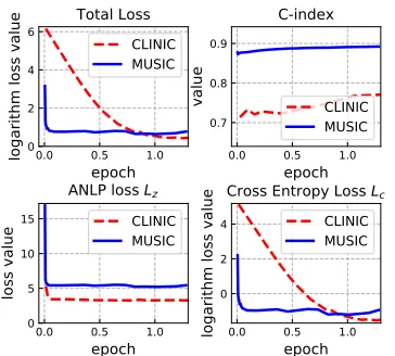
Figure 2: Learning curves. Here “epoch” means one itera-tion over the whole training data andα= 0.25in Eq. (17). Learning curves over BIDDING dataset can be referred in our supplemental material.

Model Convergence To illustrate the model training and convergence of DRSA model, we plot the learning curves and the C-index results on CLINIC and MUSIC datasets in Figure 2. Recall that our model optimizes over two loss functions, i.e., the ANLP lossLzand the cross entropy loss

Lc. From the figure, we may find that DRSA converges quickly and the values of both loss function drop to stable convergence at about the first complete iteration over the whole training dataset. Moreover, the two losses are alterna-tively optimizing and facilitate each other during the train-ing, which proves the learning stability of our model.

Model Forecasting Visualization Figure 3 illustrates the estimated survival rate curve S(t|xi_{) over time and the}

forecasted event time probabilityp(z|xi)for an arbitrarily selected test sample (xi_{, z}i_{, t}i_{). Note that the KM model}

makes the same prediction for all the samples in the dataset,

zi=67 time

0.0 0.2 0.4 0.6 0.8 1.0

S

u

rv

iv

a

l

R

a

te

S

(t

)

Survival Curve of Different Models

KM Lasso-Cox Gamma STM DeepSurv DeepHit DRSA

zi=67 time

0.00 0.05 0.10 0.15 0.20 0.25

P

ro

b

a

b

ili

ty

o

f

E

v

e

n

t

p

(z

)

Probability Curve of Different Models

KM Lasso-Cox Gamma STM DeepSurv DeepHit DRSA

Figure 3: A comprehensive visualization of survival rate

S(t|xi_{)estimation and event time probabilityp(z|x}i₎

pre-diction over different models. The vertical dotted line is the true event timezi_{of this sample.}

Table 3: Ablation study on the losses.

Models _{CLINIC MUSIC}C-index _{BIDDING CLINIC MUSIC}ANLP _BIDDING

DeepHit 0.733 0.878 0.858 5.027 5.523 5.544 DRSAunc 0.765 0.881 0.823 3.441 5.412 12.255 DRSAcen 0.760 0.882 0.900 3.136 5.459 4.990

DRSA 0.774 0.892 0.911 3.337 5.132 4.774

which is not personalized well. Our DRSA model accu-rately placed the highest probability on the true event time

zi, which explains the result of ANLP metric where DRSA achieved the best ANLP scores. Since DeepHit directly pre-dicted the probability of the event time p(zi)without any considerations of the previous conditional. And it has no supervision onto the predictions in the time range (zi, ti)

which makes the gradient signal too sparse only onto the true event timezi_{. As a result, DeepHit did not place the}

probability well over the whole time space.

Ablation Study on the Losses In this ablation study, we compare the model performance on the three losses. DRSAuncoptimizes under(Lz+Luncensored)over only the un-censored data, and DRSAcenoptimizes under(Lz+Lcensored) without the lossLuncensored. Note that our full model DRSA optimizes under all the three losses (Lz + Luncensored +

Lcensored)as stated in Eq. (17). From Table 3, we may find that both two partial likelihood lossesLuncensoredandLcensored contribute to the final prediction. Moreover, our DRSA over all the three losses achieved the best performance, which reflects the effectiveness of our classification loss Lc =

Luncensored +Lcensored as that in Eq. (16), which optimizes the C-index metric directly.

Conclusion

For the future work, it is natural to apply our model for competing risks prediction (Alaa and van der Schaar 2017; Lee et al. 2018) with shared feature embedding at the base architecture and multi-task learning for loss function.

Acknowledgments

The corresponding authors Weinan Zhang and Yong Yu thank the support of National Natural Science Foundation of China (61632017, 61702327, 61772333), Shanghai Sail-ing Program (17YF1428200).

References

Alaa, A. M., and van der Schaar, M. 2017. Deep multi-task gaus-sian processes for survival analysis with competing risks. InNIPS. Andersen, P. K.; Borgan, O.; Gill, R. D.; and Keiding, N. 2012. Statistical models based on counting processes. Springer Science & Business Media.

Bahdanau, D.; Cho, K.; and Bengio, Y. 2015. Neural machine translation by jointly learning to align and translate.ICLR. Bhattacharya, B., and Habtzghi, D. 2002. Median of the p value under the alternative hypothesis.The American Statistician. Biganzoli, E.; Boracchi, P.; Mariani, L.; and Marubini, E. 1998. Feed forward neural networks for the analysis of censored survival data: a partial logistic regression approach. Statistics in medicine 17(10):1169–1186.

Cox, D. R. 1992. Regression models and life-tables. In Break-throughs in statistics. Springer.

Faraggi, D., and Simon, R. 1995. A neural network model for survival data.Statistics in medicine.

Gordon, L., and Olshen, R. A. 1985. Tree-structured survival anal-ysis.Cancer treatment reports.

Graves, A.; Mohamed, A.-r.; and Hinton, G. 2013. Speech recog-nition with deep recurrent neural networks. InICASSP. IEEE. Grob, G. L.; Cardoso, ˆA.; Liu, C.; Little, D. A.; and Chamberlain, B. P. 2018. A recurrent neural network survival model: Predicting web user return time. InECML-PKDD.

Hochreiter, S., and Schmidhuber, J. 1997. Long short-term mem-ory.Neural computation.

Jing, H., and Smola, A. J. 2017. Neural survival recommender. In WSDM, 515–524. ACM.

Kaplan, E. L., and Meier, P. 1958. Nonparametric estimation from incomplete observations.Journal of the American statistical asso-ciation.

Katzman, J. L.; Shaham, U.; Cloninger, A.; Bates, J.; Jiang, T.; and Kluger, Y. 2018. Deepsurv: personalized treatment recommender system using a cox proportional hazards deep neural network.BMC medical research methodology18(1):24.

Khan, F. M., and Zubek, V. B. 2008. Support vector regression for censored data (svrc): a novel tool for survival analysis. InICDM. IEEE.

Knaus, W. A.; Harrell, F. E.; Lynn, J.; Goldman, L.; Phillips, R. S.; Connors, A. F.; Dawson, N. V.; Fulkerson, W. J.; Califf, R. M.; Desbiens, N.; et al. 1995. The support prognostic model: objective estimates of survival for seriously ill hospitalized adults.Annals of internal medicine.

Krizhevsky, A.; Sutskever, I.; and Hinton, G. E. 2012. Imagenet classification with deep convolutional neural networks. InNIPS.

Lao, J.; Chen, Y.; Li, Z.-C.; Li, Q.; Zhang, J.; Liu, J.; and Zhai, G. 2017. A deep learning-based radiomics model for prediction of survival in glioblastoma multiforme.Scientific reports7(1):10353. Lee, E. T., and Wang, J. 2003.Statistical methods for survival data analysis, volume 476. John Wiley & Sons.

Lee, C.; Zame, W. R.; Yoon, J.; and van der Schaar, M. 2018. Deep-hit: A deep learning approach to survival analysis with competing risks. AAAI.

Li, Y.; Wang, J.; Ye, J.; and Reddy, C. K. 2016. A multi-task learning formulation for survival analysis. InKDD.

Lisboa, P. J.; Wong, H.; Harris, P.; and Swindell, R. 2003. A bayesian neural network approach for modelling censored data with an application to prognosis after surgery for breast cancer. Artificial intelligence in medicine28(1):1–25.

Luck, M.; Sylvain, T.; Cardinal, H.; Lodi, A.; and Bengio, Y. 2017. Deep learning for patient-specific kidney graft survival analysis. arXiv preprint arXiv:1705.10245.

Mason, S. J., and Graham, N. E. 2002. Areas beneath the rel-ative operating characteristics (roc) and relrel-ative operating levels (rol) curves: Statistical significance and interpretation. Quarterly Journal of the Royal Meteorological Society.

Ranganath, R.; Perotte, A. J.; Elhadad, N.; and Blei, D. M. 2015. The survival filter: Joint survival analysis with a latent time series. InUAI, 742–751.

Ranganath, R.; Perotte, A.; Elhadad, N.; and Blei, D. 2016. Deep survival analysis. InMachine Learning for Healthcare Conference, 101–114.

Ren, K.; Zhang, W.; Chang, K.; Rong, Y.; Yu, Y.; and Wang, J. 2018. Bidding machine: Learning to bid for directly optimizing profits in display advertising.TKDE.

Tibshirani, R. 1997. The lasso method for variable selection in the cox model.Statistics in medicine16(4):385–395.

Wang, Y.; Ren, K.; Zhang, W.; Wang, J.; and Yu, Y. 2016. Func-tional bid landscape forecasting for display advertising. In ECML-PKDD.

Wang, P.; Li, Y.; and Reddy, C. K. 2017. Machine learning for survival analysis: A survey. arXiv preprint arXiv:1708.04649. Wu, W. C.-H.; Yeh, M.-Y.; and Chen, M.-S. 2015. Predicting win-ning price in real time bidding with censored data. InKDD. Zhang, H. H., and Lu, W. 2007. Adaptive lasso for cox’s propor-tional hazards model. Biometrika94(3):691–703.

Zhang, Y.; Dai, H.; Xu, C.; Feng, J.; Wang, T.; Bian, J.; Wang, B.; and Liu, T.-Y. 2014. Sequential click prediction for spon-sored search with recurrent neural networks. arXiv preprint arXiv:1404.5772.

Zhu, W. Y.; Shih, W. Y.; Lee, Y. H.; Peng, W. C.; and Huang, J. L. 2017a. A gamma-based regression for winning price estimation in real-time bidding advertising. In2017 IEEE International Confer-ence on Big Data (Big Data), 1610–1619.