A Spectral Approach for the Design of Experiments: Design,
Analysis and Algorithms
Bhavya Kailkhura [email protected]
Center for Applied Scientific Computing Lawrence Livermore National Lab Livermore, CA 94550, USA
Jayaraman J. Thiagarajan [email protected]
Center for Applied Scientific Computing Lawrence Livermore National Lab Livermore, CA 94550, USA
Charvi Rastogi [email protected]
Department of EECS
Indian Institute of Technology Bombay, MH 400076, India
Pramod K. Varshney [email protected]
Departments of EECS Syracuse University Syracuse, NY 13244, USA
Peer-Timo Bremer [email protected]
Center for Applied Scientific Computing Lawrence Livermore National Lab Livermore, CA 94550, USA
Editor:Animashree Anandkumar
Abstract
This paper proposes a new approach to construct high quality space-filling sample designs. First, we propose a novel technique to quantify the space-filling property and optimally trade-off uniformity and randomness in sample designs in arbitrary dimensions. Second, we connect the proposed metric (defined in the spatial domain) to the quality metric of the design performance (defined in the spectral domain). This connection serves as an analytic framework for evaluating the qualitative properties of space-filling designs in general. Us-ing the theoretical insights provided by this spatial-spectral analysis, we derive the notion of optimal space-filling designs, which we refer to as space-filling spectral designs. Third, we propose an efficient estimator to evaluate the space-filling properties of sample designs in arbitrary dimensions and use it to develop an optimization framework for generating high quality space-filling designs. Finally, we carry out a detailed performance comparison on two different applications in varying dimensions: a) image reconstruction and b) surro-gate modeling for several benchmark optimization functions and a physics simulation code for inertial confinement fusion (ICF). Our results clearly evidence the superiority of the proposed space-filling designs over existing approaches, particularly in high dimensions. Keywords: design of experiments, space-filling, poisson-disk sampling, surrogate model-ing, regression
c
1. Introduction
Exploratory analysis and inference in high dimensional parameter spaces is a ubiquitous problem in science and engineering. As a result, a wide-variety of machine learning tools and optimization techniques have been proposed to address this challenge. In its most generic formulation, one is interested in analyzing a high-dimensional function f :D →R defined on thed-dimensional domainD. A typical approach for such an analysis is to first create an initial samplingX ={xi∈ D}Ni=1ofD, evaluatef at allxi, and perform subsequent analysis
and learning using only the resulting tuples{(xi, f(xi))}Ni=1. Despite the widespread use of
this approach, a critical question that still persists is: how should one obtain a high quality initial sampling X for which the data f(X) is acquired or generated? This challenge is typically referred to as Design of Experiments (DoE) and solutions have been proposed as early as (Fisher, 1935) that optimized agricultural experiments. Subsequently, DoE has received significant attention from researchers in different fields (Garud et al., 2017). It is also an importantbuilding block for a wide variety of machine learning applications, such as, supervised machine learning, neural network training, image reconstruction, reinforcement learning, etc. (for a detailed discussion see Section 10). In several scenarios, it has been shown that success crucially depends on the quality of the initial samplingX. Currently, a plethora of sampling solutions exist in the literature with a wide-range of assumptions and statistical guarantees; see (Garud et al., 2017; Owen, 2009) for a detailed review of related methods. Conceptually, most approaches aim to cover the sampling domain as uniformly as possible, in order to generate the so called space-filling experimental designs (Joseph, 2016)1. However, it is well know that uniformity alone does not necessarily lead to high performance. For example, optimal sphere packings lead to highly uniform designs, yet are well known to cause strong aliasing artifacts most easily perceived by the human visual system in many computer graphics applications. Instead, a common assumption is that a good design should balance uniformity and randomness2. Unfortunately, an exact definition for what should be considered a good space-filling design remains elusive.
Most common approaches use various scalar metrics to encapsulate different notions of ideal sampling properties. One popular metric is the discrepancy of an experimental design, defined as an appropriate`p norm of the ratio of points within all (hyper-rectangular)
sub-volumes of D and the corresponding volume ratio. In other words, discrepancy quantifies the non-uniformity of a sample design. The most prominent examples of so called discrep-ancy sequencesare Quasi-Monte Carlo (QMC) methods and their variants (Caflisch, 1998). In their classical form, discrepancy sequences are deterministic though extensions to incor-porate randomess have been proposed, for example, using digital scrambling (Owen, 1995). Nevertheless, by optimizing for discrepancy these techniques focus almost exclusively on uni-formity, and consequently even optimized QMC patterns can be quite structured and create
1. The term “space-filling” is used widely in the literature on design of experiments. However, in most cases, space-filling is meant in an intuitive sense and as a synonym for “evenly or uniformly spread”. Later in this paper, we will provide a technical definition of space-filling property and what should be considered a good sample design.
aliasing artifacts. Furthermore, even the fastest known strategies for evaluating popular dis-crepancy measures require O(N2d) operations making evaluation, let alone optimization, for discrepancy difficult even for moderate dimensions. Finally, for most discrepancy mea-sures, the optimal achievable values are not known. This makes it difficult to determine whether a poorly performing sample design (e.g., in terms of generalization (or test error) in a regression application and reconstruction error in an image reconstruction application) is due to the insufficiency of the chosen discrepancy measure or due to ineffective optimization. Another class of metrics to describe sample designs are based on geometric distances. These can be used directly by, for example, optimizing the maximin or minimax distance of a sample design (Schlomer et al., 2011) or indirectly by enforcing empty disk conditions. The latter is the basis for the so-called Poisson disk samples (Lagae and Dutr, 2008), which aim to generate random points such that no two samples can be closer than a given minimal distance rmin, i.e. enforcing an empty disc of radius rmin around each sample. Typically,
Poisson-type samples are characterized by therelative radius,ρ, defined as the ratio of the minimum disk radius rmin and the maximum possible disk radius rmax for N samples to
cover the sampling domain. Similar to the discrepancy sequences, maximin and minimax designs exclusively consider uniformity, are difficult to optimize for especially in higher dimensions, and often lead to very regular patterns. Poisson disk samples useρ to trade off randomness (lowerρ values) and uniformity (higher ρ values). A popular recommendation in 2-d is to aim for 0.65≤ρ ≤0.85 as a good compromise. However, there does not exist any theoretical guidance for choosing ρ and hence, optimal values for higher dimensions are not known. As discussed in more detail in Section 2, there also exist a wide variety of techniques that combine different metrics and heuristics. For example, Latin Hypercube sampling (LHS) aims to spread the sample points uniformly by stratification, and one can potentially optimize the resulting design using maximin or minimax techniques (Jin et al., 2005).
In general, scalar metrics to evaluate the quality of a sample design tend not to be very descriptive. Especially in high dimensions different designs with, for example, the same ρ
can exhibit widely different performance and for some discrepancy sequences the optimal designs converge to random samples in high dimensions (Morokoff and Caflisch, 1994; Wang and Sloan, 2008). Furthermore, one rarely knows the best achievable value of the metric, i.e. the lowest possible discrepancy, for a given problem which makes evaluating and comparing sampling designs difficult. Finally, most metrics are expensive to compute and not easily optimized. This makes it challenging in practice to create good designs in high dimensions and with large sample sizes.
Using insights from the analysis of space-filling designs in the spectral domain, we pro-vide design guidelines to systematically trade-off uniformity and randomness for a good sampling pattern. The analytical tractability of the PCF enables us to perform theoretical analysis in the spectral domain to derive the structure of optimal space-filling designs, re-ferred to as space-filling spectral design in the rest of this paper. Next, we develop an edge corrected kernel density estimator based technique to measure the space-filling property via PCFs in arbitrary dimensions. In contrast to existing PCF estimation techniques, the proposed PCF estimator is both accurate and computationally efficient. Based on this esti-mator, we develop a systematic optimization framework and a novel algorithm to synthesize space-filling spectral designs. In particular, we propose to employ a weighted least-squares based gradient descent optimization, coupled with the proposed PCF estimator, to accu-rately match the optimal space-filling spectral design defined in terms of the PCF.
Note that there is a strong connection between the proposed space-filling spectral designs and coverage based designs such as Poisson Disk Sampling (PDS) (Gamito and Maddock, 2009). However, the major difference lies in the metric/criterion these techniques use to estimate and optimize the space-filling designs. Furthermore, existing works on PDS focus primarily on algorithmic issues, such as worst-case running times and numerical issues asso-ciated with providing high-quality implementations. However, different PDS methods often demonstrate widely different performances which raises the questions of how to evaluate the qualitative properties of different PDS patterns and how to define an optimal PDS pattern? We argue that, coverage (ρ) based metrics alone are insufficient for understanding the sta-tistical aspects of PDS. This makes it difficult to generate high quality PDS patterns. As we will demonstrate below, existing PDS approaches largely ignore the randomness objective and instead concentrate exclusively on the coverage objective resulting in inferior sampling patterns compared to space-filling spectral designs, especially in high dimensions. Note that on the other hand, the proposed PCF based metric does not have these limitations and en-ables a comprehensive analysis of statistical properties of space-filling designs (including PDS), while producing higher quality sampling patterns compared to the state-of-the-art PDS approaches.
In (Kailkhura et al., 2016a), we use the PCF to understand the nature of PDS and provided theoretical bounds on the sample size of achievable PDS. Here we significantly extend our previous work and provide a more comprehensive analysis of the problem along with a novel space-filling spectral designs, an edge corrected PCF estimator, an optimization approach to synthesize the space-filling spectral designs and a detailed evaluation of the performance of the proposed sample design. The main contributions of this paper can be summarized as follows:
• We provide a novel technique to quantify the space-filling property of sample designs in arbitrary dimensions and systematically trade-off uniformity and randomness.
• We use tools from statistical mechanics to connect the qualitative performance (in the spectral domain) of a sample design with its spatial properties characterized by the PCF.
0 0.1 0.2 0.3 0.4 0.5 0.6 0.7 0.8 0.9 1 0
0.1 0.2 0.3 0.4 0.5 0.6 0.7 0.8 0.9 1
(a) (b)
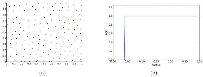
Figure 1: A sample design that balancesrandomnessanduniformity. (a) Point distribution, and (b) Pair correlation function.
• Using theoretical insights obtained via spectral analysis of point distributions, we provide design guidelines for optimal space-filling designs.
• We devise a systematic optimization framework and a gradient descent optimization algorithm to generate high quality space-filling designs.
• We demonstrate the superiority of proposed space-filling spectral samples compared to existing space-filling approaches through rigorous empirical studies on two different applications: a) image reconstruction andb) surrogate modeling on several benchmark optimization functions and an inertial confinement fusion (ICF) simulation code.
2. Related Work
In this section, we provide a brief overview of existing approaches for creating space-filling sampling patterns. Note that the prior art for this long-studied research area is too extensive to cover in detail, and hence we recommend interested readers to refer to (Garud et al., 2017; Owen, 2009) for a more comprehensive review.
2.1 Latin Hypercube Sampling
such as entropy, integrated mean square error, minimax and maximin distances, have been utilized for optimizing LHS (Jin et al., 2005). A particularly effective and widely adopted metric is the maximin distance criterion, which maximizes the minimal distance between points to avoid designs with points too close to one another (Morris and Mitchell, 1995). A detailed study on LHS and its variants can be found in (Koehler and Owen, 1996).
2.2 Quasi Monte Carlo Sampling
Following the success of Monte-Carlo methods, Quasi-Monte Carlo (QMC) sampling was in-troduced in (Halton, 1964) and since then has become the de facto solution in a wide-range of applications (Caflisch, 1998; Wang and Sloan, 2008). The core idea of QMC methods is to replace the random or pseudo-random samples in Monte-Carlo methods with well-chosen deterministic points. These deterministic points are chosen such that they are highly uni-form, which can be quantified using the measure of discrepancy. Low-discrepancy sequences along with bounds on their discrepancy were introduced in the 1960’s by Halton (Halton, 1964) and Sobol (Sobol, 1967), and are still in use today. However, despite their effective-ness, a critical limitation of QMC methods is that error bounds and statistical confidence bounds of the resulting designs cannot be obtained due to the deterministic nature of low-discrepancy sequences. In order to alleviate this challenge, randomized quasi-Monte Carlo (RQMC) sampling has been proposed (LEcuyer and Lemieux, 2005), and in many cases shown to be provably better than the classical QMC techniques (Owen and Tribble, 2005). This has motivated the development of other randomized quasi-Monte Carlo techniques, for example, methods based on digital scrambling (Owen, 1995).
2.3 Poisson Disk Sampling
While discrepancy-based designs have been popular among uncertainty quantification re-searchers, the computer graphics community has had long-standing success with coverage-based designs. In particular, Poisson disk sampling (PDS) is widely used in applications such as image/volume rendering. The authors in (Dippe and Wold, 1985; Cook, 1986) were the first to introduce PDS for turning regular aliasing patterns into featureless noise, which makes them perceptually less visible. Their work was inspired by the seminal work of Yel-lott et.al. (Yellott, 1983), who observed that the photo-receptors in the retina of monkeys and humans are distributed according to a Poisson disk distribution, thus explaining its effectiveness in imaging.
Due to the broad interest created by the initial work on PDS, a large number of ap-proaches to generate Poisson disk distributions have been developed over the last decade (Gamito and Maddock, 2009; Ebeida et al., 2012, 2011; Ip et al., 2013; Bridson, 2007; Oztireli and Gross, 2012; Heck et al., 2013; Wei, 2008; Dunbar and Humphreys, 2006; Wei, 2010; Balzer et al., 2009; Geng et al., 2013; Yan and Wonka, 2012a, 2013; Ying et al., 2013b, 2014; Hou et al., 2013; Ying et al., 2013a; Guo et al., 2014; Wachtel et al., 2014; Xu et al., 2014; Ebeida et al., 2014; de Goes et al., 2012; Zhou et al., 2012). Most Poisson disk sample generation methods are based on dart throwing (Dippe and Wold, 1985; Cook, 1986), which attempts to generate as many darts as necessary to cover the sampling domain while not violating the Poisson disk criterion. Given the desired disk size rmin (or coverage ρ), dart
to the previously accepted samples. Despite its effectiveness, its primary shortcoming is the choice of termination condition, since the algorithm does not know whether or not the do-main is fully covered. Hence, in practice, the algorithm has poor convergence, which in turn makes it computationally expensive. On the other hand, dart throwing is easy to imple-ment and applicable to any sampling domain, even non-Euclidean. For example, Anirudh et.al. use a dart throwing technique to generate Poisson disk samples on the Grassmannian manifold of low-dimensional linear subspaces (Anirudh et al., 2017).
Reducing the computational complexity of PDS generation, particularly in low and moderate dimensions, has been the central focus of many existing efforts. To this end, ap-proximate techniques that produce sample sets with characteristics similar to Poisson disk have been developed. Early examples (McCool and Fiume, 1992) are relatively simple and can be used for a wide range of sampling domains, but the gain in computational efficacy is limited. Other methods partition the space into grid cells in order to allow parallelization across the different cells and achieve linear time algorithms (Bridson, 2007). Another class of approaches, referred to astile-based methods, have been developed for generating a large number of Poisson disk samples in 2-D. Broadly, these methods either start with a smaller set of samples, often obtained using other PDS techniques, and tile these samples (Wachtel et al., 2014), or alternatively use a regular tile structure for placing each sample (Ostro-moukhov et al., 2004). With the aid of efficient data structures, these methods can generate a large number of samples efficiently. Unfortunately, these approximations can lead to low sample quality due to artifacts induced at tile boundaries and the inherent non-random na-ture of tilings. More recently, many researchers have explored the idea of partitioning the sampling space in order to avoid generating new samples that will be ultimately rejected by dart throwing. While some of these methods only work in 2−D (Dunbar and Humphreys, 2006; Ebeida et al., 2011), the efficiency of other methods that are designed for higher dimensions (Gamito and Maddock, 2009; Ebeida et al., 2012) drops exponentially with in-creasing dimensions. Finally, relaxation methods that iteratively increase the Poisson disk radius of a sample set (McCool and Fiume, 1992) by re-positioning the samples also exist. However, these methods have the risk of converging to a regular pattern with tight packing unless randomness is explicitly enforced (Balzer et al., 2009; Schlomer et al., 2011).
A popular variant of PDS is the maximal PDS (MPDS) distribution, where the maximal-ity constraint requires that the sample disks overlap, in the sense that they cover the whole domain leaving no room to insert an additional point. In practice, maximal PDS tends to outperform traditional PDS due to better coverage. However, algorithmically guaranteeing maximality requires expensive checks causing the resulting algorithms to be slow in moder-ate (2-5) and practically unfeasible in higher (7 and above) dimensions. Though strmoder-ategies to alleviate this limitation have been proposed in (Ebeida et al., 2012), the inefficiency of MPDS algorithms in higher dimensions still persists. Interestingly, a common limitation of all existing MPDS approaches is that there is no direct control over the number of samples produced by the algorithm, which makes the use of these algorithms difficult in practice, since optimizing samples for a given sample budget is the most common approach.
and connect the proposed metric (defined in the spatial domain) to the quality metric of design performance (defined in the spectral domain).
3. A Metric for Assessing Space-filling Property
(a) Random (b) Regular (c) Sobol (d) Halton
(e) LHS (f) MPDS (g) Step PCF (h) Stair PCF
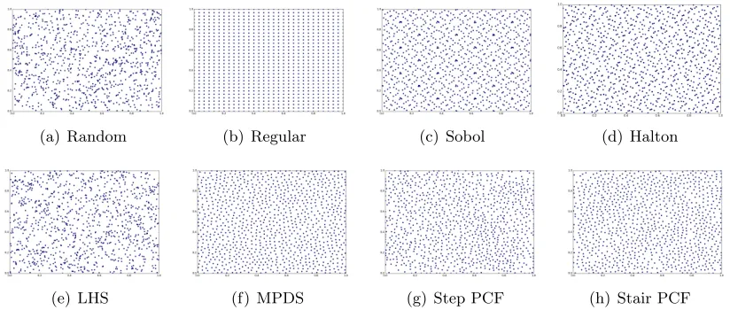
Figure 2: Visualization of 2-d point distributions obtained using different sample design techniques. In all cases, the number of samplesN was fixed at 1000.
(a) Random (b) Regular (c) Sobol (d) Halton
(e) LHS (f) MPDS (g) Step PCF (h) Stair PCF
Figure 3: Space-filling Metric: Pair correlation functions, corresponding to the samples in Figure 2, characterize the coverage (and randomness) of point distributions obtained using different techniques.
(a) Random (b) Regular (c) Sobol (d) Halton
(e) LHS (f) MPDS (g) Step PCF (h) Stair PCF
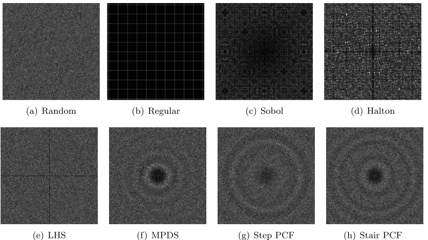
Figure 4: Performance Quality Metric: Power spectral density is used to characterize the effectiveness of sample designs, through the distribution of power in different frequencies.
3.1 Space-filling Designs
Without any prior knowledge of the function f of interest, a reasonable objective when creating X is that the samples should be random to provide an equal chance of finding features of interest, e.g., local minima in an optimization problem, anywhere inD. However, to avoid sampling only parts of the parameter space, a second objective is to cover the space inDuniformly, in order to guarantee that all sufficiently large features are found. Therefore, a good space-filling design can be defined as follows:
Definition 1 A space-filling design is a set of samples that are distributed according to a uniform probability distribution (Objective 1: Randomness) but no two samples are closer than a given minimum distance rmin (Objective2: Coverage).
Next, we describe the metric that we use to quantify the space-filling property of a sample design. The proposed metric is based on the spatial statistic, pair correlation function (PCF) and we will show that this metric is directly linked to the quality metric of design performance defined in the spectral domain.
3.2 Pair Correlation Function as a Space-filling Metric
of the intensity λand product density β of a point process (Illian et al., 2008; Oztireli and Gross, 2012).
Definition 2 Let us denote the intensity of a point processX asλ(X), which is the average number of points in an infinitesimal volume around X. For isotropic point processes, this is a constant value. To define the product densityβ, let{Bi} denote the set of infinitesimal
spheres around the points, and {dVi} indicate the volume measures of Bi. Then, we have3
P r(X1 = x1,· · ·,XN =xN) =β(x1,· · · ,xN)dV1· · ·dVN which represents the probability
of having points xi in the infinitesimal spheres {Bi}. In the isotropic case, for a pair of
points, β depends only on the distance between the points, hence one can writeβ(xi,xj) =
β(||xi−xj||) =β(r) and P r(r) =β(r)dVidVj. The PCF is then defined as
G(r) = β
λ2. (1)
Note that the PCF characterizes spatial properties of a sample design. However, in several cases, it is easier to link the quality metric of a sample design to its spectral properties. Therefore, we establish a connection between the spatial property of a sample design defined in PCF space to its spectral properties.
3.3 Connecting Spatial Properties and Spectral Properties of Space-filling Designs
Fourier analysis is a standard approach for understanding the qualitative properties of sampling patterns. Hence, we propose to analyze the spectral properties of sample designs, using tools such as the power spectral density, in order to assess their quality. For isotropic samples, a quality metric of interest is the radially-averaged power spectral density, which describes how the signal power is distributed over different frequencies.
Definition 3 For a finite set ofN points, {xj}Nj=1, in a region with unit volume, the power
spectral density of the sampling function PN
j=1δ(x−xj) is formally defined as P(k) = 1
N|S(k)| 2= 1
N
X
j,`
e−2πik.(x`−xj), (2)
where |.|denotes thel2-norm andS(k) denotes the Fourier transform of the sampling func-tion.
The radially-averaged power spectral density (PSD) is denoted usingP(k). Next, we show that the connection between spectral properties of a d-dimensional isotropic sample design and its corresponding pair correlation function can be obtained via thed-dimensional Fourier transform or more efficiently using the 1-d Hankel transform.
Proposition 4 For an isotropic sample design withN points,{xj}Nj=1, in ad-dimensional
region with unit volume, the pair correlation function G(r) and radially averaged power spectral densityP(k) are related as follows:
G(r) = 1 + V
2πNH[P(k)−1] (3)
where V is the volume of the sampling region and H[.] denotes the 1-d Hankel transform, defined as
H(f(k)) =
Z ∞
0
kJ0(kr)f(k)dk,
with J0(.) denoting the Bessel function of order zero.
Proof Note that PSD and PCF of a sample design are related via thed-dimensional Fourier transform as follows:
P(k) = 1 +N
V F(G(r)−1)
= 1 +N
V
Z
Rd
(G(r)−1) exp(−ik.r)dr.
It can be shown that, for radially symmetric or isotropic functions, the above relationship simplifies to
P(k) = 1 + 2πN
V H[G(r)−1].
Next, using the inverse property of the Hankel transform, i.e.,
H0−1(f(r)) =
Z ∞
0
rJ0(kr)f(r)dr,
we have
G(r) = 1 + V
2πNH[P(k)−1]. (4)
Proposition 4 is important as it enables us to qualitatively understand space-filling designs by first mapping them into the PCF space constructed based on spatial distances between points and, then, evaluating and understanding spectral properties of sample designs.
In Figure 3, we show the PCF4 of some commonly used 2-d sample designs (N = 1000) illustrated in Figure 2. As can be observed, both regular grid samples and QMC sequences have significant oscillations in their PCFs, which can be attributed to their structured nature. Regular grid sample design demonstrates a large disk radius rmin (G(r) = 0 for
0 ≤ r ≤ rmin) as every sample is at least rmin apart from the rest of the samples, which
in turn implies a better coverage. However, in practice, they perform poorly (e.g., in terms of generalization (or test error) in regression application and reconstruction error in image reconstruction application) compared to randomized sample designs and this can
be understood by studying their spectral properties. In contrast, random sample (Monte-Carlo) designs have a constant PCF with nearly no oscillations, since point samples are uncorrelated, thus, P(r) = λdxλdy and theoretically have G(r) = 1, ∀r. Furthermore, the LHS design has a similar PCF as random designs with the exception of a small, yet non-zero,rmin.
Other variants of PDS like MPDS, Step PCF and Stair PCF designs attempt to trade-off between coverage (G(r) = 0 for 0 ≤ r ≤ rmin) and randomness G(r) = 1, for r > rmin.
Note that the Step and the Stair PCF methods are space-filling spectral designs proposed later in this paper. However, upon a careful comparison, it can be seen that MPDS has a larger peak and more oscillations in its PCF compared to the proposed designs. In fact, our empirical studies show that the amount of oscillations in the PCF of the MPDS design significantly increases with dimensions.
Next, in Figure 4, we show the corresponding PSDs of the different sample designs. It can be seen that, oscillations in PCF directly correspond to oscillations in PSDs. For example, the oscillatory behavior of the PCF for regular and QMC sequences cause a non-uniform distribution of power in their corresponding PSDs. Furthermore, the larger peak height in the PCF of MPDS implies that a large amount of power is concentrated in a small frequency band instead of power being distributed over all frequencies. In Section 5, we will analyze the effect of the shape of PCF on the performance of a sample design in detail.
It is important to note that, not every PCF (or PSD) is physically realizable by a sample design. In fact, there are two necessary mathematical conditions 5 that a sample design must satisfy to be realizable.
Definition 5 (Realizability) A PCF can be defined to be potentially realizable through a sample design, if it satisfies the following conditions:
• its PCF must be non-negative, i.e., G(r)≥0, ∀r, and
• its corresponding PSD must be non-negative, i.e., P(k)≥0, ∀k.
As both the PSD and the PCF characteristics are strongly tied to each other (as shown in Proposition 4), these two conditions limit the space of realizable space-filling spectral designs. The results from this section will serve as tools for qualitatively understanding and, thus, designing optimal space-filling spectral designs in the following sections.
4. Space-filling Spectral Designs
In this section, we first formalize desired characteristics of a good space-filling design, as given in Definition 1. Next, we will describe the proposed framework for creating space-filling spectral designs.
Definition 6 A set X of N random samples {Xi}Ni=1 in a sampling domain D can be
characterized as a space-filling design, if X = {Xi = xi ∈ D; i = 1,· · ·N} satisfy the
following two objectives:
• ∀Xi ∈ X, ∀4D ⊆ D : P r(Xi =xi∈ 4D) = R
4DdX
• ∀xi,xj ∈ X : ||xi−xj|| ≥rmin
where rmin is referred to as the coverage radius.
In the above definition, the first objective states that the probability of a random sample
Xi ∈ X falling inside a subset 4D of D is equal to the hyper-volume of 4D (uniform
distribution). The second condition enforces the minimum distance constraint between point sample pairs for improving coverage.
A Poisson design enforces the first condition alone, in which case the number of samples that fall inside any subset4D ⊆ D obeys a discrete Poisson distribution. Though easier to implement, Poisson sampling often produces distributions where the samples are grouped into clusters and leaves holes in possibly the regions of interest. In other words, this in-creases the risk of missing important features, when only the samples are used for analysis. Consequently, a sample design that distributes random samples in a uniform manner across
D is preferred, so that clustering patterns are not observed. The coverage condition ex-plicitly eliminates the clustering behavior by preventing samples from being closer than
rmin. A space-filling design can be defined conveniently in the PCF domain and we refer to
this as the space-filling spectral design, due to its direct connection to the spectral domain properties.
4.1 Defining a Space-filling Spectral Design in Spatial Domain
For Poisson design, point locations are not correlated and, therefore,P(r) =λdxλdy. This implies that for Poisson designs G(r) = 1. Similarly, for space-filling designs, due to the minimum distance constraint between the point sample pairs, we do not have any point samples in the region 0≤r < rmin. Consequently, space-filling spectral designs are defined
as a step pair correlation function in the spatial domain (Step PCF).
Proposition 7 Given the desired coverage radius rmin, a space-filling spectral design is defined in the spatial domain as
G(r−rmin) =
0 if r < rmin 1 if r ≥rmin.
As a consequence of Proposition 4, space-filling spectral designs can equivalently be defined in the spectral domain.
4.2 Defining a Space-filling Spectral Design in Spectral Domain
We derive the power spectral density of the space-filling spectral design using the connection established in Section 3. Following our earlier notation, we denote thed-dimensional power spectral density by P(k) andd-dimensional PCF byG(r).
D of volume V, can be defined in the PSD domain as
P(k) = 1−N V
2πrmin k
d2
Jd
2(krmin)
where Jd
2
(.) is the Bessel function of orderd/2.
Proof We know that,
P(k) = 1 +N
V F(G(r)−1), (5)
= 1 +N
V
Z
Rd
(G(r)−1) exp(−ik.r)dr, (6)
where F(.) denotes the d-dimensional Fourier transform. Note that for the radially sym-metric or isotropic functions, i.e., G(r) wherer =||r||, the above relationship simplifies to
P(k) = 1 +N
V (2π) d
2k1−
d
2Hd
2−1
rd2−1(G(r)−1)
, (7)
where
Hv(f(r))(k) =
Z ∞
0
rJv(kr)f(r)dr
is the 1−d Hankel transform of order v with J being the Bessel function. To derive the PSD of a step function, we first evaluate the Hankel transform of f(r) = rd2−1(G(r)−1) whereG(r) is a step function.
Hd
2−1
rd2−1(G(r)−1)
=
Z ∞
0
rd2Jd
2−1(kr) (G(r)
−1)dr
= −
Z rmin
0
rd2Jd
2−1 (kr)dr
= −
r
d
2 min
k Jd2
(krmin)
Using this expression in (7), we obtain
P(k) = 1−N V
2πrmin k
d2
Jd
2(krmin). (8)
5. Qualitative Analysis of Space-filling Spectral Designs
In this section, we derive insights regarding the qualitative performance of space-filling spectral designs. To this end, we analyze the impact of the shape of the PCF on the reconstruction performance. Further, for a tractable analysis, we consider the task of re-covering the class of periodic functions using space-filling spectral designs and analyze the reconstruction error as a function of their spectral properties. The analysis presented in this section will clarify how the shape of the PCF of a sample design directly impacts its reconstruction performance.
5.1 Analysis of Reconstruction Error for Periodic Functions
Let us denote the Fourier transform of the sample designX by S. The function to be sam-pled and its corresponding Fourier representation are denoted by I and ˆI(k) respectively. Now, the spectrum of the sampled function is given by ˆIs(k) =S ∗Iˆ(k). Note that a
sam-pling pattern with a finite number of points is comprised of two components, a DC peak at the origin and a noisy remainder ¯S. Thus, equivalently, we have ˆIs(k) ={N δ(k)+ ¯S}∗Iˆ(k).
The error introduced in the process of function reconstruction is the difference between the reconstructed and the original functions:
E(k) =|Iˆs(k)/N− I(k)|2 =|S ∗¯ Iˆ(k)/N|2
where we have divided the R.H.S. byN to normalize the energy ofIs. For error analysis, we focus on the low frequency content of the error term, since the high frequency components are removed during the reconstruction process.
Denoting the power spectrum without the DC component by ¯P(k), for a constant func-tion the error simplifies to
E(k)∝ |S¯(k)|2 ∝P¯(k). (9) This, as stated above, allows for the characterization of the error in terms of the spectral properties of the sampling pattern used.
Next, we consider an important class of functions, the family of periodic functions, for further analysis. All periodic functions with a finite period can be expressed as a Fourier series6, which is a summation of sine and cosine terms
I(x) =a0+
M X
m=1
amcos(2πmx) + M X
m=1
bmsin(2πmx).
The Fourier transform of this function is equivalently a summation of pulses:
ˆ
I(k) =a0δ(k) +
M X m=1 am 1
2(δ(k−m) +δ(k+m)
+ M X m=1 bm 1
2(δ(k+m)−δ(k−m))
.
Making substitutions,am+bm=Am, am−bm=Bm, we obtain
E(k) = 1 4N2
4a0
¯
S(k) +
M X
m=1
AmS¯(k+m) +BmS¯(k−m)
2 .
The reconstruction error can then be upper bounded as follows:
E(k)≤ 1
4N
h
4a20P¯(k) +
M X
m=1
A2mP¯(k+m) +B2mP¯(k−m)
i
. (10)
In the case of a single sinusoidal function, cos(2πf x), using triangle inequality, this be-comes (Heck et al., 2013)
E(k)≤ 1
4N
h
¯
P(k+f) + ¯P(k−f) + 2
q
¯
P(k+f) ¯P(k−f)
i
. (11)
Even though this is only an upper bound and the theoretic analysis is restricted to periodic functions, we have empirically found that it accurately predicts the characteristics of the sampling error for a broad range of complex functions and provides useful guidelines (more details are provided in Section 9).
The above analysis implies that to assess the quality of the sample designs, one can analyze their spectral behavior. More specifically, the above analysis suggests that to min-imize the reconstruction error (Eq. (10) and (11)): (a) the power spectra of the sample design should be close to zero, and (b) for errors to be broadband white noise (uniform over frequencies), the power spectra should be a constant. Note that in several applications, e.g., image reconstruction, most relevant information is predominantly at low frequencies. In such scenarios, this naturally leads to the following criteria for sample designs: (a) the spectrum should be close to zero for low frequencies which indicates the range of frequencies that can be represented with almost no error, (b) the spectrum should be a constant for high frequencies or contain minimal amount of oscillations in the power spectrum. However, as we will see next, there exist a trade-off between low frequency power and high frequency oscillations in power spectra.
5.2 Effect of PCF Characteristics on Sampling Performance
Based on the two criteria discussed above, we assess the effect of the shape of the PCF on the quality of space-filling designs in the spectral domain. Note that PCFs of the samples constructed in practice (Figure 2) often demonstrates the following characteristics: (a) presence of a zero-region characterized by rmin, (b) a large peak around rmin, and (c)
damped oscillations. To model and analyze these characteristics, we consider the following parametric PCF family7
G(r;rmin, δ, a, c) =G(r−rmin) + (a−1) (G(r−rmin)−G(r−rmin−δ)) (12)
+a−1
4r exp(−r/2) sin(c×r−c)G(r−rmin)
where G(r−rmin) is the Step function, peak width δ ≥0 and the peak height a≥1 and
last term in (12) corresponds to damped oscillations. This family is a generalization of Step PCF, with additional parameterization of peak height and oscillations in the PCF.
5.2.1 Effect of Peak Height on Spectral Properties
In order to study the impact of increasing peak height in the PCF on the PSD characteristics, we conduct an empirical study. We compute the PSD of a sample design with the following parameters: N = 195, rmin = 0.02, δ = 0.005. Note that we vary the PCF peak height a,
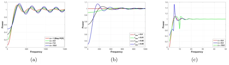
which actually reflects the behavior of existing coverage based PDS algorithms. As shown in Figure 5(a), increasingaresults in both significantlyhigher low frequency power andlarger high frequency oscillations. As expected, the PSD of the Step PCF (ora= 1) performs the best, i.e., the spectrum is close to zero for low frequencies and constant for high frequencies.
5.2.2 Effect of Disk Radius on Spectral Properties
Next, we study the importance of choosing an appropriatermin (or coverageρ) while
gener-ating sample distributions. In Figure 5(b), we show the PSD for N = 195 and a= 1, with varying disk radius values rmin. For a fixed sample budget, as we increase the radius, we
observe two contrasting changes in the PSD: (i) the spectrum tends to be close to zero at low frequencies and (ii) an increase in oscillations for high frequencies. Consequently, there is a trade-off between low frequency power and high frequency oscillations in power spectra which can be controlled by varying rmin. However, the increase in oscillations are less
sig-nificant compared to the gain in the zero-region. Furthermore, in several applications, low frequency content is more informative, and hence one may still attempt to maximize rmin
or coverage.
5.2.3 Effect of Oscillations on Spectral Properties
Finally, we study the effect of oscillations in the PCF on the power distribution in the spectral domain. In Figure 5(c), we plot the PSD for a = 1 with varying amounts of oscillations controlled via the parameter c. It can be seen that introducing oscillations in the PCF results in significantly higher low frequency power and larger high frequency oscillations. As expected, the PSD of the Step PCF (orc= 0) behaves the best.
In summary, the discussion in this section suggests that the PCF of an ideal space-filling spectral design should have the following three properties: (a) large rmin, (b) small peak
height, and (c) low oscillations. Since, the Step PCF satisfies these three properties, it is expected to be a good space-filling spectral design. Next, we consider the problem of optimizing the parameter of the Step PCF design, i.e. rmin.
6. Optimization of Step PCF based Space-filling Spectral Designs
The proposed space-filling metric enjoys mathematical tractability and is supported by theoretical results as defined in Section 4. This enables us to obtain new insights for optimizing Step PCF based space-filling spectral designs. In particular, (a) For a fixedrmin,
(a) (b) (c)
Figure 5: (a) Effect of peak height in the PCF on power spectra, (b) Effect of disk radius in the PCF on power spectra, (c) Effect of oscillations in the PCF on power spectra.
fixed sampling budget N, we derive the maximum achievable rmin in arbitrary dimension d.
6.1 Case 1: Fixed rmin
The problem of finding the maximum number of point samples in a Step PCF based space-filling spectral design with a given disk radiusrmin can be formalized as follows:
maximize N
subject to P(k)≥0, ∀k
G(r−rmin)≥0, ∀r,
(13)
whereP(k) = 1−N V
2πrmin k
d2
Jd
2(krmin). Note that a space-filling spectral design has to satisfy realizability constraints as defined in Definition 5.
Proposition 9 (Kailkhura et al., 2016a) For a fixed disk radiusrmin, the maximum number of point samples possible for a realizable Step PCF based space-filling spectral design in the sampling region with volumeV can be approximated as
N ≈ VΓ
d
2 + 1
πd2rd min
.
Proof Using the definition of the Step PCF function, the constraintG(r−rmin) is trivially
satisfied. Note that the constraint P(k) ≥0, ∀k is equivalent to min
words,
min
k 1−ρ
2πrmin k
d2
Jd
2(krmin)
≥0
⇔ max
k ρ
2πrmin k
d2
Jd
2(krmin)
≤1
⇔ ρ(2π)d2 rd
minmax
k
Jd
2
(krmin)
(krmin) d
2
!
≤1
⇔ ρ(2π)d2 rd
min
1
2d2Γ d
2+ 1
.1 (14)
⇔ N . VΓ
d
2+ 1
(π)d2 rd
min
where, in (14) we have used the fact that Jv(x)≈(x/2)v/Γ(v+ 1) andρ=N/V.
Note that for the 2-dimensional case, we have J1(krmin)
krmin = jinc(krmin) where jinc(.) is the sombrero function (sometimes called besinc function or jinc function). Now using the fact that jinc(x) has the maximum value equal to 1/2, for a fixed disk radiusrmin, the maximum
number of point samples possible in a 2-d Step PCF based space-filling spectral design is given by
N =V /π(rmin)2,
which again corroborates our bound in Proposition 9.
6.2 Case 2: Fixed N
Alternately, we can also derive the bound for the disk radius of Step PCF with a fixed sampling budget N as follows:
maximize rmin
subject to P(k)≥0, ∀k
G(r−rmin)≥0, ∀r
(15)
Proposition 10 (Kailkhura et al., 2016a) For a fixed sampling budget N, the maximum possible disk radius rmin for a realizable Step PCF based space-filling spectral design in the sampling region with volumeV can be approximated as
rmin≈
d
s
VΓ d2 + 1
πd2N
.
6.3 Relative Radius of Step PCF
As mentioned before, the current literature characterizes coverage by the fraction ρ of the maximum possible radius rmax forN samples to cover the sampling domain, such that
rmin =ρrmax. The maximum possible disk radius is achieved by the deterministic hexagonal
lattice (Schreiber, 1943) and can be approximated in a d dimensional sampling region as
rmax ≈
d
q Ad
CdN. Here,Ad is the hypervolume of the sampling domain and Cd=Vd/r
dwith
Vdbeing the hypervolume of a hypersphere with radiusr. Note that a uniformly distributed
point set can have a relative radius of 0, and the relative radius of a hexagonal lattice equals 1 (in 2-d). Next, we derive a closed-form expression for the relative radius of Step PCF based design.
Proposition 11 For a fixed sampling budget N, the maximum relative radius ρ for Step PCF based space-filling spectral design in the sampling region with volume V is given by
ρ= 1 2 √dη
d
where ηd is maximal density of a sphere packing in d-dimensions.
Proof Let us denote byrmax= arg min r
ηd, then, the maximal density of a sphere packing
withN samples ind-dimensions is given by
ηd=
N πd/2
Γ(1 +d2)
rd max
V (16)
⇔ ηd=
rmax
rmin
d
(17)
⇔ ρ= 1 2 √dη
d
(18)
where equality in (17) uses Proposition (10).
For d= 2 and 3, the relative radius simplifies to:
ρ= 0.52
s
π√3
6 , ford= 2, and
ρ= 0.53
s
π√2
6 , ford= 3.
Note that finding the maximal density of a sphere packing for an arbitrary high dimen-sion (except ind= 2,3 and recently in 8,24 (viazovska, 2017; Cohn et al., 2017)) is an open problem. Note that best known packings are often lattices, thus, we use the best known lattices to be an approximation ofrmax in our analysis8.
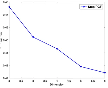
In Figure 6, we plot the relative radius ρ = rmin/rmax of Step PCF for different
di-mensions d. It is interesting to notice that the relative radius of Step PCF based designs
Figure 6: Relative radiusρ=rmin/rmax of Step PCF based space-filling spectral design for
different dimensionsd.
increases as the dimensiondincreases, i.e., Step PCF based designs approach a more regu-lar pattern. Further, note that for a fixed sampling budget bothrmin and rmax increase as
the number of dimensions increases. The Step PCF based designs maintain randomness by keeping the PCF flat, but this comes at a cost: the disk radiusrmin of these patterns is very
small (as can be seen from Figure 6). For several applications, covering the space better (by trading-off randomness) is more important. In the next section, we will propose a new class of space-filling spectral designs that can achieve a much higherrmin at the small cost
of compromising randomness by introducing a single peak into an otherwise flat PCF.
7. Space-filling Spectral Designs with Improved Coverage
To improve the coverage of Step PCF base space-filling spectral design, in this section, we propose a novel space-filling spectral design which systematically trades-off randomness with coverage of the resulting samples. Note that the randomness property can be relaxed either by increasing the peak height of the PCF, or by increasing the amounts oscillations in the PCF (as discussed in Section 5.2). For simplicity9, we adopt the former strategy and use only the peak height parameter. More specifically, as an alternative to Step PCF, we design the following generalization which we refer as the Stair PCF design.
7.1 Stair PCF based Space-filling Spectral Design
Now, we define the proposed Stair PCF based space-filling design and quantify the gains achieved in the coverage characteristics (i.e. rmin).
Stair PCF in the Spatial Domain: The Stair PCF construction is defined as follows:
G(r;r0, r1, P0) =f(r−r1) +P0(f(r−r0)−f(r−r1)), (19)
withf(r−r0) =
0 ifr≤r0
1 ifr > r0
,
wherer0 ≤r1 and P0≥1.
This family of space-filling spectral designs has three interesting properties:
• except for a single peak in the region r0 ≤ r ≤ r1, the PCF is flat, thus, does not
compromise randomness entirely,
• both the height and width of the peak can be optimized to maximize coverage,
• the Step PCF based spectral design can be derived as as a special case of this con-struction.
Now, the problem boils down to finding the combinations of the three parameters (r0, r1, P0)
that are realizable and yield a good sample design (discussed in Section 7.2). A represen-tative example of Stair PCF is shown in Figure (7(a)).
Stair PCF in the Spectral Domain: Following the analysis in the earlier sections, we derive the power spectral density of Stair PCF based space-filling spectral designs.
Proposition 12 The power spectral density of a Stair PCF based space-filling spectral de-signs, G(r;r0, r1, P0), withN samples in the sampling region with volume V is given by
P(k) = 1−N V P0
2πr0 k
d2
Jd
2(kr0)
−N
V (1−P0)
2πr1 k
d2
Jd
2(kr1).
Proof Using results from Section 4.2, we have
P(k) = 1 +N
V (2π) d
2k1−
d
2Hd
2−1
rd2−1(G(r)−1)
. (20)
To derive the PSD of a Stair function, we first evaluate the Hankel transform of f(r) = (G(r)−1) whereG(r) is a Stair function.
Hd
2−1
rd2−1(G(r)−1)
=
Z ∞
0
rd2Jd
2−1(kr) (G(r)
−1)dr
=−P0
Z r0
0
rd2Jd 2−1
(kr)dr−(1−P0)
Z r1
0
rd2Jd 2−1
(kr)dr
=−P0
r
d
2 0
k Jd2
(kr0)−(1−P0)
r
d
2 1
kJd2 (kr1)
Using this expression in (20),
P(k) = 1−N V P0
2πr0 k
d2
Jd
2(kr0)
−N
V (1−P0)
2πr1 k
d2
Jd
Radius (r)
PC
F
(a) (b) d= 2 (c)d= 3
(d) d= 4 (e)d= 5 (f)d= 6
Figure 7: (a) Pair correlation function of Stair PCF based designs, (b)-(f) Maximum Disk Radius For Step and Stair PCF for dimensions 2 to 6.
Next, we empirically evaluate the gain in coverage achieved by Stair PCF based designs compared to the Step PCF based designs.
7.2 Coverage Gain with Stair PCF
Ideally, the optimal Stair PCF should be obtained by simultaneously maximizing r0 (:= rmin) and minimizingP0. Furthermore, not all PCFs in the Stair PCF family are realizable.
Due to the realizability conditions, the parameters cannot be adjusted independently. The main challenge, therefore, is to find the combinations of the three parameters (r0, r1, P0) that
is realizable and yield a good sample design. Unlike Step PCF, the closed form expression for the optimal parameters (r0, r1, P0) are difficult to obtain, and, therefore, we explore this
family of PCF patterns empirically by searching configurations for which:
• the disk radius r0 is as high as possible, and
• the PCF is flat with minimal increase in the peak height P0.
7.2.1 Disk Radius rmin vs. Sample Budget N
In this section, we show the increase in coverage (or rmin) obtained by compromising
ran-domness by increasing peak height in the PCF. We constrain the peak height to be below
P0 ≤1.5 and analyze the gain in rmin due to this small compromise in randomness.
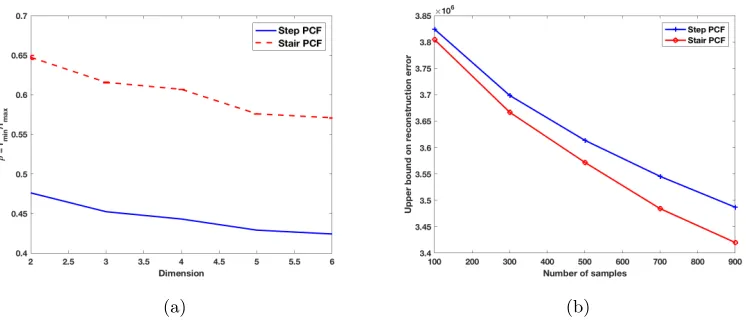
(a) (b)
Figure 8: (a) Gain in the relative radius ρ achieved with the Stair PCF constructions, in comparison to the Step PCF constructions; (b) Upper bound on the reconstruc-tion error of Step and Stair PCF based construcreconstruc-tions.
through 7(f), we compare the maximumrmin achieved by the Step and Stair PCF designs,
for varying sample sizes in dimensions 2 to 6. It can be seen that introducing a small peak in the PCF results in a significant increase in the coverage. This gain can be observed for all sampling budgets in all dimensions. Furthermore, as expected, for low sampling budgets maximal gain is observed, and should decrease with increasing N as the rmin for both the
families will asymptotically (inN) converge to zero.
7.2.2 Relative Radius ρ vs. Dimension d
In this section, we study the increase in relative radiusρ due to the introduction of a peak in the PCF. Again, we assume thatP0≤1.5,rstepmin≤r0 ≤2×rminstep and r0 ≤r1 ≤1.5×r0.
In Figure 8(a), we show the maximumρ=rmin/rmax achieved by the Step and Stair PCFs
for different dimensions d. For Stair PCF, we do not have a closed form expression of ρ, thus, we obtain the maximum achievablermin empirically for various sampling budgets and
plot the mean (with standard deviation) behavior of theρ. It can be seen that introducing a small peak in the PCF results in a significant increase in the relative radius. This gain can be observed at all sampling budgets in all dimensions. This also corroborates the recommendation of using 0.65≤ρ≤0.85 in practice for coverage based designs and suggests that in higher dimensionsρ should be higher.
7.2.3 Analysis of Reconstruction Error Upper Bound
increase in the sampling budget. More interestingly, the reconstruction error of Stair PCF is lower compared to the reconstruction error of Step PCF, thus showing the effectiveness of increased coverage in sample designs.
8. Synthesis of Space-filling Spectral Designs
In this section, we describe the proposed approach for synthesizing sample designs that match the optimal (Stair or Step) PCF characteristics. Existing approaches for PCF match-ing such as (Oztireli and Gross, 2012; Kailkhura et al., 2016b) rely on kernel density esti-mators to evaluate the PCF of a point set. A practical limitation of these approaches is the lack of an efficient PCF estimator in high dimensions. More specifically, these estimators are biased due to lack of an appropriate edge correction strategy. This bias in PCF estimation arises due to the fact that sample hyper-spheres used in calculating point-pattern statistics may fall partially outside the study region and will produce a biased estimate of the PCF unless a correction is applied. The effect of this bias is barely noticeable in 2 dimensions and hence existing PCF matching algorithms have ignored this. However, this problem be-comes severe in higher dimensions, thus, making the matching algorithm highly inaccurate. To address this crucial limitation, we introduce an edge corrected estimator for computing the PCF of sample designs in arbitrary dimensions. Following this, we describe a gradient descent based optimization technique to synthesize samples that match the desired PCF.
8.1 PCF Estimation in High Dimensions with Edge Correction
In order to create an unbiased PCF estimator, we propose to employ an edge corrected kernel density estimator, defined as follows:
ˆ
G(r) = VW
γW
VW
N
1
SE(N−1) N X
i=1
N X
j=1
i6=j
k(r− |xi−xj|) (22)
wherek(.) denotes the kernel function; here we use the classical Gaussian kernel
k(z) = √1 πσ exp
− z 2
2σ2
. (23)
In the above expression,VW indicates the volume of the sampling region. When the sampling
region is a hyper-cube with length 1, we have VW = 1. Let SE denote the area of
hyper-sphere with radius r which is given by
SE =
drd−1πd2 Γ(1 + d2).
Also, we denote the surface area of the sampling region bySW, which is expressed as
The term VW
γW performs edge correction to handle the unboundedness of the estimator,
whereγW is an isotropic set covariance function given by
γW =
1
SE
Z
0≤φd−1≤2π 0≤φi≤π,i=1 tod−2
SWγdφ1· · ·dφd−1 (24)
whereγ =Qd
p=1(1− |xp|) with
x1 =rcosφ1 x2 =rsinφ1cosφ2 x3 =rsinφ1sinφ2cosφ3
.. .
xd−1=rsinφ1· · ·sinφd−2cosφd−1 xd=rsinφ1· · ·sinφd−2sinφd−1.
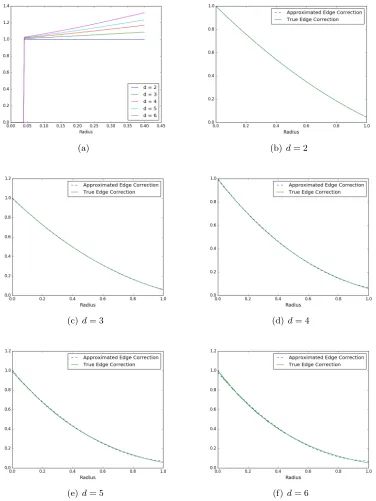
In Figure 9(a), we show that by using an approximate edge correction factor (using the same factor asd= 2), the PCF is wrongly estimated. Moreover, as the dimension increases, the estimated PCF moves farther away from the true PCF very quickly.
Note that the calculation of the correct edge correction factor requires the evaluation of a multi-dimensional integral which is computationally expensive in high dimensions. In this paper, we provide a closed form approximation of γW (using polynomial regression of
order 2) in different dimensions d = 2 to 6 when r ≤1.0. More specifically, we have the following approximation ˆγW = 1−a1r+a2r2 wherea1 and a2 are as given below.
Dimension d= 2 d= 3 d= 4 d= 5 d= 6
a1 4/π 1.47 1.63 1.75 1.89 a2 1/π 0.54 0.72 0.87 1.04
It can be observed from Figures 9(b) through 9(f) that the proposed approximations are quite tight.
8.2 Synthesis Algorithm
The underlying idea of the proposed algorithm is to iteratively transform an initial random input sample design such that its PCF matches the target PCF. In particular, we propose a non-linear least squares formulation to optimize for the desired space-filling properties. Let us denote the target PCF byG∗(r). We discretize the radius r into m points {rj}mj=1
and minimize the sum of the weighted squares of errors between the target PCF G∗(rj)
and the curve-fit function (kernel density estimator of PCF) G(rj) over m points. This
scalar-valued goodness-of-fit measure is referred to as the chi-squared error criterion and can be posed as a non-linear weighted least squares problem as follows.
arg min
M X
j=1
G(rj)−G∗(rj)
wj
2
(a) (b) d= 2
(c)d= 3 (d) d= 4
(e)d= 5 (f)d= 6
wherewj indicates the weight (importance) assigned to the fitting error at radius rj. This
optimization problem can be efficiently solved using a variant of gradient descent algorithm (discussed next), that in our experience converges quickly. In the simplest cases of uniform weights the solution tends to produce a higher fitting error at lower radii rj. To address
this challenge we use a non-uniform distribution for the weights {wj}. These weights are
initialized to be uniform and are updated in an adaptive fashion in the gradient descent iterations. The weightwj at gradient descent iterationt+ 1 is given by (Kailkhura et al.,
2016b):
wj =
1
|Gt(r
j)−G∗(rj)|
where Gt(rj) is the value of the PCF at radius rj during the gradient descent iteration t.
Note that PCF matching is a highly non-convex problem. We found that the following trick further helps solve PCF matching problem more efficiently.
8.2.1 One Sided PCF Smoothing
We propose to perform one sided smoothing of the target PCF which is given as follows:
ˆ
G∗(r) =
(cr)b ifr < r
min
1 ifr≥rmin.
where c is some pre-specified constant and b > 1 is the smoothing constant obtained via cross-validation. More specifically, we add polynomial noise in the low radius region of the PCF. This can also be interpreted as polynomial approximation of the PCF in the low radii regime. We have noticed that sometimes adding a controlled amount of Gaussian noise instead of polynomial noise also improves the performance.
8.2.2 Edge Corrected Gradient Descent
The non-linear least squares problem is solved iteratively using gradient descent. Starting with a random point set X = {xi}Ni=1, we iteratively update xi in the negative gradient
direction of the objective function. At each iteration k, this can be formally stated as
xki+1 =xki −λ ∆i |∆i|
,
where λ is the step size and ∆i = {∆ki}dk=1 in the normalized edge corrected gradient is
given by
∆pi =X
i6=l
(xpl −xpi)
|xl−xi| m X
j=1
G(rj)k−G∗(rj)
wj(1−a1rj+a2r2j)rd
−1
j
(|xl−xi| −rj)k(rj− |xi−xl|). (25)
We re-evaluate the PCF G(rj)k of the updated point set after each iteration using the
unbiased estimator from the previous section.
Algorithm 1 Space-filling Spectral Sample Design using PCF Matching Algorithm
1: Input: Number of samplesN, dimensiond, Smoothed target PCF ˆG∗(rj), weightswj,
step sizeλ, edge correction factors (a1, a2)
2: X←Random(N, d) . Initial random sample design
3: G←PCF(X) .Calculate initial PCF using Eq. (22)
4: fort= 1 to T do .TotalT gradient descent iterations
5: for i= 1 to N do . Update each sample at a time
6: ∆pi ← ∂ ∂xpi
M P
j=1
Gt(rj)−G∗(rj)
wj
2
forp∈ {1,· · ·, d} .Calculate gradients
using (25)
7: xti+1←xti−λ ∆i |∆i|
.Update the sample
8: Gt←PCF(X) . Update the PCF
9: wj ←
1
|Gt(r
j)−Gˆ∗(rj)|
. Update weights
10: return X . Space-filling Spectral Samples
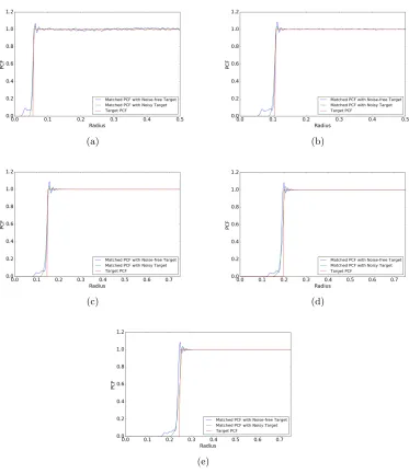
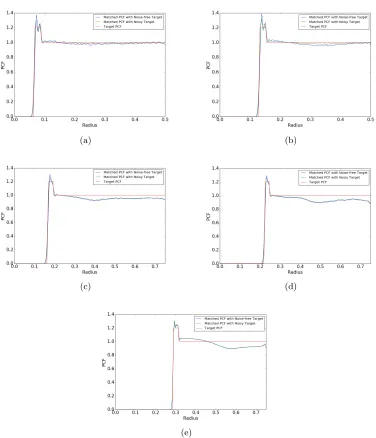
In Figure 10, we compare the behavior of the proposed PCF matching algorithm with and without the one sided PCF smoothing. The target PCF is designed using a Step PCF design with rmin as given in Proposition 10. PCF matching is carried out with varying
sampling budget, N = 100, 200, 400, 600, 800 for d = 2, 3, 4, 5, 6, respectively. The variances of the Gaussian kernel were set at σ2 = 0.0065, 0.007, 0.01, 0.01, 0.01 for
d = 2, 3, 4, 5, 6, respectively and the step size for the gradient descent algorithm was fixed at 0.001. The value of b was obtained using cross-validation. The initial point set was generated randomly (uniform) in the unit hyper-cube and matching was carried for 100 gradient descent iterations. It can be observed that the proposed algorithm produces an accurate fit to the target, and that the smoothing actually leads to improved performance.
In Figure 11, we demonstrate the synthesis of a Stair PCF based spectral design, using parameters P0 = 1.2, δ= 0.025. Similar to the previous case, PCF matching is carried out
(a) (b)
(c) (d)
(e)
Figure 10: Step PCF synthesis using one sided PCF smoothing technique. (a) d = 2 (b)
d= 3 (c)d= 4 (d)d= 5 (e) d= 6.
9. Experiments
al-(a) (b)
(c) (d)
(e)
Figure 11: Stair PCF synthesis using one sided PCF smoothing technique. (a) d= 2 (b)
d= 3 (c)d= 4 (d)d= 5 (e) d= 6.
gorithms difficult in practice. However, the proposed approach can control both N and
rmin simultaneously. For our qualitative comparison, we perform three empirical studies,
Table 1: Impact of different space-filling designs on image reconstruction performance. In all cases, we show the reconstructed images and their PSNR values.
α Sobol Halton LHS MPDS Step Stair
0.001
14.82 dB 15.75 dB 14.29 dB 16.90 dB 16.00 dB 16.46 dB
0.002
12.10 dB 12.34 dB 11.39 dB 13.16 dB 12.58 dB 12.96 dB
0.003
11.22 dB 11.38 dB 10.75 dB 11.88 dB 11.55 dB 11.78 dB
0.004
10.61 dB 10.67 dB 10.34 dB 10.92 dB 10.80 dB 10.90 dB
0.005
9.80 dB 9.70 dB 9.59 dB 9.82 dB 9.83 dB 9.84 dB
0.006
9.09 dB 8.97 dB 8.97 dB 8.96 dB 9.08 dB 9.02 dB
0.007
9.1 Image Reconstruction
In this experiment, we consider the problem of designing sample distributions for image reconstruction. More specifically, we consider the commonly used zone plate test function:
z(r) = (1 + cos(αr2))/2,
with varying levels of complexity (or frequency content) α. Note that we choose the zone plate for our study over natural images, since it shows the response for a wide range of frequencies and aliasing effects that are not masked by image features. For all zone plate renderings in this paper, we have tiled toroidal sets of 1000 2-dimensional points over the image-plane and utilized a Lanczos filter with a support of width 4 for resampling. Further, we also report the peak signal-to-noise ratio (PSNR) as a quantitative error measure:
PSNR = 20 log10 1 MSE,
where MSE is the mean squared error. However, it is well known in the image processing community that PSNR can be a weak surrogate for visual quality (as we will see later) and, therefore, we also show the reconstructed images.
Table 1 illustrates the reconstructions obtained using different space-filling designs, for varying values ofα. It can be observed from the results that the QMC sequences produce a large amount of aliasing artifacts in the high frequency regions, which can be directly linked to the oscillations in their corresponding PCFs. On the other hand, LHS design recovers a small amount of low-frequencies, and maps most of the frequencies to white noise due to its small rmin and near-constant PCF. In contrast, sample designs which attempt to trade-off
between coverage and randomness properties, i.e., MPDS and the proposed spectral space-filling designs (as seen in Figure 3), have superior reconstruction quality. These designs reduce the aliasing artifacts, have cleaner low frequency content (upper left corner)) and map all high frequencies (bottom right corner) to white noise. More interestingly, we see that for low complexity cases, i.e., lower α, the MPDS performs the best followed by the proposed Stair and Step PCF respectively. For moderately complex images, the Stair PCF performs the best followed by the Step and the MPDS. Finally, for highly complex images, the Step PCF performs the best followed by the Stair and the MPDS. These observations corroborate our discussion in Section 5.2 that an increase in rmin (coverage) in the PCF
results in an increase in the range of low frequencies that can be recovered without aliasing, and equivalently reduction in the amount of oscillations (or an increase in randomness) in the PCF leads to reduced oscillations in the PSD, which in turn indicates a systematic mapping of high frequency content to white noise. Note that when α = 0.007, both LHS and Sobol designs have PSNR greater than (or equal to) the PSNR of Step PCF design. However, the quality of the reconstructed image by Step PCF is far superior compared to the one by LHS and Sobol designs. This further corroborates our claim on PSNR being a weak surrogate and justifies the use of reconstructed images itself as a performance metric.
9.2 Regression Modeling for Benchmark Optimization Functions
performance. More specifically, we consider a set of benchmark analytic functions between dimensions 2 and 6, that are commonly used in global optimization tests (Jamil and Yang, 2013). They are chosen due to their diversity in terms of their complexity and shapes. We compare the performance of proposed space-filling spectral designs (Step, Stair) with cov-erage based designs (MPDS), low-discrepancy designs (Halton and Sobol), latin hypercube sampling and random sampling. Appendix A lists the set of functions used in our exper-iments. In each case, we fit a random forest regressor with 30 trees and repeated for 20 independent realizations of sample designs. We evaluate the generalization performance on 106 regular grid based test samples. Finally, we report mean (horizontal lines) and standard deviation (vertical lines) of 3 popular quality metrics (over 20 realizations) to quantify the performance of the resulting regression models: mean squared error (MSE), relative average absolute error (AAE), and the R2-statistic. The metrics are defined as follows:
M SE(y,yˆ) =
PN
i=1(yi−yˆi)2
N , (26)
AAE(y,yˆ) =
PN
i=1|yi−yˆi|
N∗ST D(y) , (27)
R2(y,yˆ) = 1−
PN
i=1(yi−yˆi)2
PN
i=1(yi−M EAN(y))2
(28)
wherey=f(x) are the true function values and ˆy are the predicted values.
Tables 2 through 6 show the performance of different space-filling designs for various analytic functions in dimensions 2 to 6, respectively10. We see that, ford= 2 (Table 2), LHS and Halton sequences perform better compared to the rest of the sample designs on most of the test functions. However, on some functions, e.g., GoldsteinPrice, Stair PCF and MPDS perform better. Therefore, none of the sample designs consistently guarantee superior performance. For d= 3 (Table 3), we see that Stair PCF design and MPDS (followed by Sobol sequences) perform consistently better compared to the rest of the approaches. As we go higher in dimensions, i.e., d > 3, we notice a significant gain in the performance of Stair PCF based space-filling spectral designs. Interesting, the amount of performance gain of Stair PCF based design increases as we go higher in dimensions. The reason for the poor regression performance of QMC sequences and LHS for d > 3 is due to their poor space-filling properties in high dimensions (Wang and Sloan, 2008). In comparison, both space-filling spectral designs and MPDS have good space-filling properties. We found that Stair PCF design and MPDS have similar coverage characteristics (rmin). However,
the difference in their performance can be attributed to the fact that MPDS designs have significantly more oscillations in their PCF compared to an equivalent Stair PCF based space-filling spectral design, i.e. violation of the randomness objective.
Table 2: Impact of sample design on generalization performance of regression models fit to benchmark analytical functions in 2 dimensions. LHS and Halton sequences perform slightly better compared to rest of the sample designs.
Function MSE AAE R2-Statistic
GoldsteinPrice
Chichinadze
Rosenbrock
Cube
9.3 Surrogate Model Design for an Inertial Confinement Fusion (ICF) Simulator
In this subsection, we consider the problem of designing surrogate models for an inertial confinement fusion (ICF) simulator developed at the National Ignition Facility (NIF). The NIF is aimed at demonstrating inertial confinement fusion (ICF), that is, thermonuclear ignition and energy gain in a laboratory setting. The goal is to focus 192 beams of the most energetic laser built so far onto a tiny capsule containing frozen deuterium. Under the right conditions, the resulting pressure will collapse the target to the point of ignition where hydrogen starts to fuse and produce massive amounts of energy, effectively creating a small star which can be harnessed for energy production. Though significant progress has been made, the ultimate goal of “ignition” has not yet been reached.
Table 3: Impact of sample design on generalization performance of regression models fit to benchmark analytical functions in 3 dimensions. While the Stair PCF and MPDS designs are consistently better than the other methods, the amount of performance gain is minimal.
Function MSE AAE R2-Statistic
BoxBetts
Hartmann3
Wolfe
Helical Valley
considered here is a so called engineering or macro-physics simulation ensemble in which an implosion is simulated using different input parameters, such as, laser power, pulse shape etc. From these simulations, scientists extract a set of drivers, physical quantities believed to determine the behavior of the resulting implosion. These drivers are then analyzed with respect to the energy yield to better understand how to optimize future experiments. As one can expect, the success of this pipeline heavily depends on the quality of samples used for post-shot simulations.