Learning Representations of Persistence Barcodes
Christoph D. Hofer [email protected]
Department of Computer Science University of Salzburg
Salzburg, Austria
Roland Kwitt [email protected]
Department of Computer Science University of Salzburg
Salzburg, Austria
Marc Niethammer [email protected]
Department of Computer Science University of North Carolina Chapel Hill, NC, USA
Editor:Michael Mahoney
Abstract
We consider the problem of supervised learning with summary representations of topological features in data. In particular, we focus on persistent homology, the prevalent tool used in topological data analysis. As the summary representations, referred to as barcodes or per-sistence diagrams, come in the unusual format of multi sets, equipped with computationally expensive metrics, they can not readily be processed with conventional learning techniques. While different approaches to address this problem have been proposed, either in the context of kernel-based learning, or via carefully designed vectorization techniques, it remains an open problem how to leverage advances in representation learning via deep neural networks. Appropriately handling topological summaries as input to neural networks would address the disadvantage of previous strategies which handle this type of data in atask-agnostic manner. In particular, we propose an approach that is designed to learn a task-specific representation of barcodes. In other words, we aim to learn a representation that adapts to the learning problem while, at the same time, preserving theoretical properties (such as stability). This is done by projecting barcodes into a finite dimensional vector space using a collection of parametrized functionals, so called structure elements, for which we provide a generic construction scheme. A theoretical analysis of this approach reveals sufficient conditions to preserve stability, and also shows that different choices of structure elements lead to great differences with respect to their suitability for numerical optimization. When implemented as a neural network input layer, our approach demonstrates compelling performance on various types of problems, including graph classification and eigenvalue prediction, the classification of 2D/3D object shapes and recognizing activities from EEG signals.
Keywords: Topological data analysis, persistent homology, topological summary, super-vised learning, deep learning
c
1. Introduction
Over the past decade, concepts from the field of algebraic topology have evolved into computationally efficient algorithms to analyze data. Methods from this field are now succinctly summarized under the term topological data analysis (TDA) (Carlsson, 2009) and have found a broad range of applications, ranging from studying activity patterns of the visual cortex (Singh et al.,2008), breast cancer (Nicolau et al.,2011), the manifold of natural image patches (Carlsson et al., 2008), to analyzing brain artery trees (Bendich et al., 2016), 3D surfaces (Reininghaus et al.,2015; Li et al., 2014;Hofer et al., 2017b), clustering (Chazal et al.,2013b) and the recognition of 2D object shapes (Turner et al., 2014b). Arguably, the most prevalent method used in practice is persistent homology (see Edelsbrunner et al.,
2002;Zomorodian and Carlsson, 2004) which offers a concise summary representation of
topological features in data. In short, persistent homology tracks topological changes as we analyze data at multiple “scales”. As the scale changes, topological features (i.e., connected components, holes, etc.) appear and disappear. Persistent homology associates a lifespan to these features, resulting in a multi set of (birth, death) tuples, typically visualized as a barcode or apersistence diagram. Thesetopological signatures can offer complementary information that is not easily extractable by other methods. This opens up novel pathways to address learning problems based on topological information.
Despite the advantages of TDA in capturing topological invariants of data, the field is still largely disconnected from recent developments in machine learning. With respect to persistent homology, this can be attributed to the unusual data structure underlying topological signatures, that is, multi sets, and the associated (computationally intensive) metrics in that space. In fact,Mileyko et al.(2011) andTurner et al.(2014a) have investigated the theoretical properties of this metric space and shown that it is not easily amenable to statistical computations (for example, there is no unique Fr´echet mean), or machine learning for that matter. Nevertheless, several works (see Section3) have recently shown advances towards bridging the gap between machine learning and TDA; either in the context of kernel-based learning, or via suitable vectorization techniques for persistence diagrams / barcodes, based on algebraic ideas. However, both strategies typically come at the cost of computational complexity. In case of vectorization techniques, computational bottlenecks typically arise when computing the vectorization itself. In case of kernels, it is well-known that kernel-based learning (such as SVMs) scales poorly with sample size and sometimes even the kernel computation itself can be computationally challenging. Importantly, both strategies rely on an a-priorifixed representation of topological signatures.
With respect to the latter issue, the success of deep neural networks in vision (seeKrizhevsky et al., 2012; He et al., 2016; Huang et al., 2017), or natural language processing (see
PH(K, f)
Vθ0
D1 i
Dji
DM i
Vθj
Out:xji ∈RN
VθS
learnable
fixed
In: Multi set
Neural
Net
w
o
rk
(e.g.,
MLP
,
RNN,
etc.)
Θ
Input data objectsoi Point clouds 2D/3D object shape Graphs/Networks . . .
Persistence barcodes Task-specific vectorization
K Simplicial complex of data object
f Filtration function
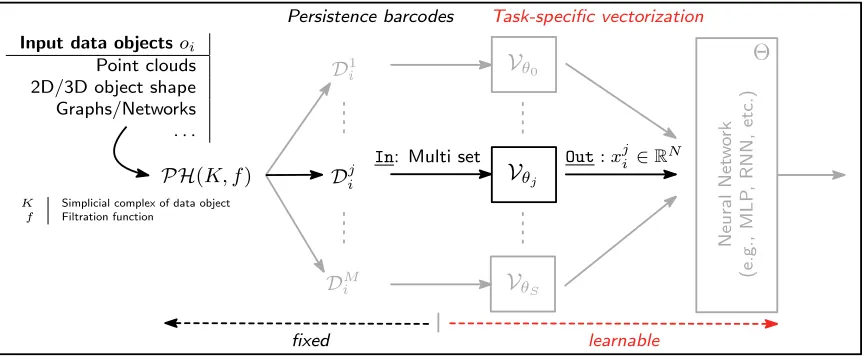
Figure 1: Illustration oflearnable, task-specific vectorizations of barcodes. Inputs are bar-codesDji, obtained by (1) constructing a simplicial complexK from data objectoi
and (2) computing persistent homology (PH) of a filtration ofK. The superscript j inDji denotes that we can have multiple barcodes per oi, e.g., considering
ho-mology groups of different dimension, or from multiple filtrations. Each barcode is amulti set, fed to one (or more) parametrized (by θj) input layers that implement
a mapping Vθj to R
N. These vectorizations are then fed to a neural network
implementing, e.g., a discriminant classifier.
Contributions. This work extends Hofer et al. (2017a), where we introduced a neural network layer that can handle barcodes in a principled manner. The core idea is to project points in a barcode by a collection of parametrized functionals, so called structure elements. The parametrization is learned during training and allows to obtain a task-specific vectorization of barcodes (see Figure1). In this work, we conduct an in-depth theoretical analysis of this approach. In particular, we prove that such a construction leads to an induced mapping of barcodes that is continuous with respect to the p-Wasserstein distance, although it cannot be stable with respect to p-Wasserstein for p > 1. This complements a similar recent result ofReininghaus et al. (2015) in the context of kernels. Further, we show that the original strategy of Hofer et al. (2017a) to enforce the required conditions on structure elements has limitations and present an alternative allowing a broader range of functional families to be considered. This then enables us to introduce new structure elements with desirable properties for learning. Finally, we present experiments on a variety of problems, including graph classification, eigenvalue prediction of (normalized) graph Laplacian matrices, 2D/3D shape recognition and the classification of EEG signals.
2. Background
For brevity, we only provide a brief overview of the mathematical concepts relevant to this work and refer the reader toHatcher (2002) or Edelsbrunner and Harer(2010) for details.
Homology. The key idea of homology theory is to study the properties of some object X by means of (commutative) algebra. In particular, we assign toX a sequence of modules Cn which are connected by homomorphisms∂n, that is,
· · · ∂3
−−−−−→C2
∂2
−−−−−→C1
∂1
−−−−−→C0
∂0
−−−−−→0
with
∂n:Cn→Cn−1 such that im∂n⊆ker∂n−1 .
A structure of this form is called a chain complex and by studying its homology groups
Hn= ker∂n/im∂n+1 we can derive properties ofX.
A prominent example of a homology theory issimplicial homology. Throughout this work, it is the used homology theory and hence we will now concretize the already presented ideas. Let K be a simplicial complex and Kn its n-skeleton. Then, we set Cn(K) as the vector
space generated (freely) byKn overZ/2Z1. The connecting homomorphisms
∂n:Cn(K)→Cn−1(K)
are called boundary operators. For an-simplexσ = [x0, . . . , xn]∈Kn, we define them as
∂n(σ) = n
X
i=0
[x0, . . . , xi−1, xi+1, . . . , xn]
and linearly extend this to Cn(K), that is, ∂n(
P
σi) =
P
∂n(σi).
Persistent homology. LetK be a simplicial complex. A sequence of simplicial complexes, (Ki)m
i=0, such that
∅=K0⊆K1⊆ · · · ⊆Km=K
is called afiltration of K. If we use the extra information provided by the filtration of K, we obtain the following sequence of chain complexes
· · · C1
2 C11 C01 0
· · · C2
2 C12 C02 0
· · · Cm
2 C1m C0m 0
∂3
ι ∂2
ι ∂1
ι ∂0
∂3
ι ∂2
ι ∂1
ι ∂0
∂3 ∂2 ∂1 ∂0
where Ci
n=Cn(Kni), ιdenotes the inclusion and 0 is the trivial group. To illustrate this
more conveniently, we provide a simpleexample:
K1
A B
⊆ K2
C D
E
⊆ K3
F G
H I
v2
v1
v3 v4
The chain groups in this example are as follows:
ForK1
C01 = [[v1],[v2]]Z2
C11 =0 C21 =0
ForK2
C02 = [[v1],[v2],[v3]]Z2 C12 = [[v1, v3],[v2, v3]]Z2
C22 =0
For K3
C03 = [[v1],[v2],[v3],[v4]]Z2 C13 = [[v1, v3],[v2, v3],[v3, v4]]Z2
C23 =0 This then leads to the concept of persistent homology groups, defined by
Hni,j = ker∂ni/(im∂nj+1∩ker∂ni) for i≤j .
The ranks, βni,j = rankHni,j, of these homology groups (that is, the n-th persistent Betti
numbers), capture the number of homological features of dimensionality n (for example, connected components forn= 0, holes for n= 1, etc.) that persist from ito (at least) j. In fact, according to (Edelsbrunner and Harer, 2010, Fundamental Lemma of Persistent Homology), the quantities
µi,jn = (βni,j−1−βni,j)−(βni−1,j−1−βni−1,j) for i < j (1) encode all the information about the persistent Betti numbers of dimensionn. Before we continue to introduce barcodes, we take a short detour and discuss the concept of multi sets, a data structure that appears naturally when encoding information captured by persistent homology.
Multi sets. We focus on multi sets over a fixed domain. Informally, multi sets extend the concept of ordinary sets by allowing elements to occur more than once. For example, in the multi setM ={1,1,2}, the element 1 is contained 2 times. For multi sets over a fixed domain,D, this concept can be formalized by following the idea thatordinary sets over a fixed domain can be represented by their indicator function. Analogously, we can represent a multi set by its multiplicity function. Hence, a multi setM can be interpreted as a function
M :D→N∞0 =N∪ {0,∞} ,
where M(x) =n denotes thatx is contained in M n-times. However, we will write
multM(x) instead of M(x)
Definition 1 Let M, N be multi sets and A an ordinary set over the domainD. We adhere to the following conventions:
(M1) supp(M) = supp(multM) ={x∈D: multM(x)>0} Support
(M2) x∈M ⇔x∈supp(M) Set membership
(M3) |M|=P
x∈supp(M)multM(x) Cardinality
(M4) (M]N)(x) = multM]N(x) = multM(x) + multN(x) Union
(M5) (M∩A)(x) = multM∩A(x) = multM(x)·1A(x) Intersection with set
(M6) (M\A)(x) = multM\A(x) = multM(x)·1D\A(x) Difference to set
(M7) Letf :D→Rn; then, P
x∈M
f(x) = P
x∈supp(M)
multM(x)·f(x) Function evaluation
If necessary, we can always interpret an ordinary set as a multi set, since the characteristic function can be interpreted as a multiplicity function with values in{0,1}.
Topological signatures. A typical way to obtain a filtration of a simplicial complex K is to consider sub level sets of a real valued function,f :K→R , defined on K such that for
ρ∈K and the corresponding boundary operator,∂, it holds that
f(σ)≤f(ρ) for σ ∈∂(ρ) .
Let
a1 <· · ·< am withm=|f(K)|
be the sorted sequence of values of f(K). Then, we obtain (Ki)m
i=0 by setting K0 =∅ and Ki =f−1 (−∞, ai]
for 1≤i≤m .
If we construct a multi set such that, fori < j, the point (ai, aj) is inserted with multiplicity
µi,jn , see Eq. (1), we effectively encode the persistent homology of dimensionnwith respect
to the sub level set filtration induced by f.
Definition 2 (Barcode) Let Ω ={(b, d)∈R2:d > b} the upper-diagonal part of the real plane. A barcode, D, is a multi set, over the domain Ω. We denote by D the set of all barcodes with finite cardinality.
Remark 3 While, in theory, barcodes are not necessarily finite, in any practical setup where data is analyzed, we deal with barcodes of finite cardinality. Thus, in all subsequent parts of this work, we assumeD ∈D.
For a given complexK of dimensionnmax and a functionf (of the discussed form), we can interpret persistent homology (PH) as a mapping
(K, f)7−−→PH (D0, . . . ,Dnmax−1) , where Di is the barcode of dimensioniand n
EquippingDwith a metric structure, allows studying the sensitivity of PHto perturbations
inK orf. Before we can give the definitions of the metrics usually used for this purpose, we have to introduce the concept of relative bijective matchings between two multi sets.
Definition 4 (∆-relative bijective matchings between finite multi sets) LetM, N
be finite multi sets over the domain D. Further, let ∆⊂D such that
supp(M)∩∆ =∅ and supp(N)∩∆ =∅ .
A ∆-relative bijective matching between M, N is a multi set, ϕ, over D×Dsuch that
(C1) supp(ϕ)∩(∆×∆) =∅ ,
(C2) ∀x∈supp(M) : P
(x,y)∈supp(ϕ)
multϕ (x, y)
= multM(x), and
(C3) ∀y∈supp(N) : P
(x,y)∈supp(ϕ)
multϕ (x, y)
= multN(y) .
Intuitively, multϕ (x, y)
=nmeans thatxis matched toy n-times. Condition(C1)ensures that there are no matchings from ∆ to ∆, while(C2) and(C3) ensure thatx, y are used in a matching exactly as often as they are contained inM,N.
Definition 5 (Bottleneck, Wasserstein distance) Let(R2, δ) be a metric space and let
∆ ={(x, y)∈R2 :x=y}
be the diagonal of the real plane. For two barcodes D,E ∈ D, the Bottleneck (wδ∞) and Wasserstein (wδ
p) distances (with respect to the metricδ) are defined by
wδ
∞(D,E) = infϕ sup
(x,y)∈supp(ϕ) δ(x, y)
and
wδp(D,E) = inf
ϕ
X
(x,y)∈supp(ϕ)
multϕ (x, y)
·δ(x, y)p
1 p
withp∈[1,∞) ,
where the infimum is taken over all ∆-relative bijective matchings ϕbetween D and E.
Remark 6 In the case where δ is the metric induced by the q-norm, k · kq, we write w∞ for wk·k∞
∞ and wqp for w k·kq
p .
We also remark that introducing the Wasserstein distances as in Definition 5, using ∆-relative bijective matchings, deviates from the original formulation inCohen-Steiner et al.
(2007). However, this variant simplifies any of our subsequent analyses of stability/continuity properties involving those metrics. We refer the reader to (Cohen-Steiner et al., 2007, 2010;
Chazal et al., 2009) for a selection of existing stability results in a broader context and further details.
Remark 7 By setting µi,n∞ = βni,m−βni−1,m, we extend Eq. (1) to features which never
{(b, d)∈R×(R∪ {∞}) :d > b}. However, if the filtration of K is defined by the sub level sets of a function f, a more pragmatic way of handling essential features is to map their death time to the maximum of the function f. In many cases, for example height filtrations, this has a more natural interpretation (see Section6.3).
3. Related work
In order to deal with the practical inconveniences associated to a (direct) handling of barcodes in machine learning problems, several strategies have been proposed over the last couple of years. On a high level, these approaches can be categorized into (1) kernel-based
techniques and (2) approaches that aim for a vectorization. Next, we summarize these techniques, draw connections between them, and elaborate on how they relate to our work. We additionally discuss related research on learning with (multi) set data structures and highlight important differences to our approach.
Kernel-based techniques. In short, the idea of kernel-based learning techniques (Sch¨olkopf and Smola, 2001) is to rely on a positive-definitekernel function k:X × X →Rthat realizes
an inner producthφ(x), φ(y)iG =k(x, y), forx, y∈ X, in a Hilbert spaceGfor some (possibly unknown) feature mapping φ:X → G. A kernel can either be constructed by (1) defining a functionk that captures some notion of similarity between two input objects and showing its positive-definiteness, or (2) by explicitly constructingφand using the inner product inG
as a kernel (that is positive-definite by construction). Both strategies have found application in the context of kernel-based learning with topological signatures.
As a representative of the latter strategy,Reininghaus et al.(2015) introduced thepersistence scale-space (PSS) kernel. The construction is based on first representing a diagram as a sum of Dirac deltas and then using this representation as the initial condition of a heat-diffusion process with a Dirichlet boundary condition on the diagonal ∆. The solution of this partial differential equation (at timet) resides in L2(Ω) and serves as an explicit feature mapping. The inner-product in L2(Ω) is then used as a kernel function. A different, yet conceptually similar approach is taken by Bubenik (2015) to construct persistence landscapes, that is, functions of the formλ:N×R→R∪ {+∞,−∞}. Upon the definition of a suitable norm k·kp onN×R, landscapes map barcodes into a (separable) Banach spaceLp(N×R). Notably,
forp= 2, we get the Hilbert spaceL2(
N×R) which then facilitates to use the inner-product
again to define a kernel. InKwitt et al. (2015), it is further shown that under some mild restrictions on the barcodes (that is, birth-death boundedness and an upper-bound on the multiplicities of points), an exponentiated version of the persistence scale-space kernel is universal2 (Steinwart and Christmann,2008, Def. 4.52). A similar argumentation would give a universal kernel constructed from persistence landscapes, forp= 2. When working in this setting, statistical computations (seeGretton et al., 2012) become feasible, although, for landscapes many theoretical properties for statistics have already been developed (Chazal et al.,2013a,2014;Fasy et al.,2014).
A different kernel-based technique is introduced by Kusano et al. (2016), where the authors leverage the theory of reproducing kernel Hilbert space (RKHS) embeddings of probability measures (see Berlinet and Thomas-Agnan,2004). Different to Reininghaus et al.(2015), a diagram is represented as a weighted measure, that is, a weighted sum of Dirac deltas, centered at each point of the diagram. The weighting function accounts for the different persistence of each point. Notably, the authors show stability of the kernel-induced distance between barcodes with respect to the Hausdorff distance (for two compact metric spaces embedded in the same metric space). Essentially, this is achieved via the aforementioned weighting function. Contrary to that,Reininghaus et al.(2015) achieve stability by enforcing the Dirichlet boundary condition on the diagonal. In the latter case, this only leads to stability of the kernel-induced distance with respect to wq1 and it is shown that no kernel for which k(F ] G,D) =k(F,D) +k(G,D) holds (with F,G,D ∈D), is stable with respect to
wqp forp >1.
The recently proposed kernel approach of Carri´ere et al. (2017) follows the strategy of directly defining k, instead of explicitly constructing a feature mapφ. While there is strong indication (via counterexamples) that the negative of the wqp distance cannot be used in a
construction of the form k(F,G) = exp(−wqp(F,G)), as wqp is not negative semi-definite, the
authors circumvent this problem by introducing the sliced Wasserstein distance which can be shown to be negative semi-definite. The distance induced by the resulting kernel, termed thesliced Wasserstein kernel, is strongly equivalent to w∞1 .
Vectorization techniques. A conceptually different line of developments is to “coordina-tize” the barcode space which allows vectorization. In (Adcock et al.,2016), for example, the authors define a ring of algebraic functions on the space of barcodes. A similar approach with appealing properties is based on tropical algebraic geometry (Kali˘snik Verov˘sek, 2018). In particular, the coordinatizations in the latter work are stable with respect to wqp and
w∞ (which is not the case for the approach by Adcock et al. (2016)) and facilitates the
development of sufficient statistics for barcodes (Monod et al.,2017). While this presents a promising approach, the challenge is to construct suitable polynomials in a computationally efficient manner.
Another instance of a vectorization technique is presented inAdams et al. (2017), where barcodes are mapped to so-calledpersistence surfaces. This is done by computing a weighted sum of normalized (isotropic) Gaussians, evaluated at each point in the diagram. Upon discretization of this persistence surface, one obtains thepersistence image that can then be vectorized and fed to, for example, a linear SVM. Notably, a similar approach, motivated from a statistical point of view, was introduced by Chen et al. (2015) based on earlier ideas presented in Edelsbrunner et al.(2012). Similar to Kusano et al. (2016), stability of persistence images (with respect to w∞1 ) is achieved via a continuous piecewise-differentiable weighting function that evaluates to zero on the diagonal ∆. By taking a measure-theoretic point of view,Chazal and Divol(2018) have recently shown that, in a wide range of situations, the persistence surface is a kernel density estimator for the expected barcode.
example, PCA, or a discriminant classifier. However, it is unclear how the hyper-parameter N should be chosen appropriately, a choice that will most likely depend on the application.
In summary, most vectorization and kernel-based techniques retain certain stability properties of persistence diagrams / barcodes with respect to the common metrics in the field of persistent homology. Yet, they also share one common drawback: the mapping of the topological signatures to a representation that is compatible with existing learning techniques ispre-defined. While this is, a-priori, not a disadvantage for statistical computations, it can be undesirable for learning, as the representation isagnosticto the learning task. In fact, the success of deep neural networks (seeKrizhevsky et al., 2012; He et al.,2016) has shown that
learning representations is a preferable approach. It is worth pointing out that algebraic constructions (Adcock et al.,2016;Kali˘snik Verov˘sek,2018;Monod et al.,2017) might be amenable to learning task-specific representations, but it is unclear if this is computationally feasible. Furthermore, techniques based on kernels, such as (Reininghaus et al., 2015; Kwitt et al.,2015;Kusano et al.,2016;Carri´ere et al.,2017), additionally suffer scalability issues as training kernel SVMs scales poorly with the number of samples (Chapelle,2007) and even evaluating the kernel function itself can be computationally challenging. In the spirit of end-to-end training, we therefore aim for a computationally efficient approach that allows to learn a task-specific representation.
Learning with sets. As mentioned earlier, learning with barcodes requires to appropriately handle multi sets and to respect the topology induced by the metrics. In the context of deep learning, using multi sets as input has gained limited attention so far, except for approaches where the multi set is the prediction target (Welleck et al., 2017). On the other hand, learning with sets as input to neural networks has spawned considerable research interest recently. InQi et al.(2017a,b), for instance, the authors primarily focus on handling point clouds in a way that is permutation invariant with respect to the points. Zaheer et al.
(2017) present a characterization theorem for valid set functions that allow the design of appropriate neural networks layers. In particular, it is shown that if set elements are from a countable domain, a necessary condition for a function to be a valid set function is to have a decomposition of the form ρ(P
x∈Sφ(x)), for a suitable choice of ρ andφ. In the
uncountable case, this was only shown to hold for sets of fixed size, but it is conjectured that the previous characterization holds even for sets of arbitrary size. In this work, we are exactly in the latter setting, as we consider multi sets over an uncountable subset ofR2 as
input. Moreover, the fact that we are dealing with multi sets and a topology induced by the metrics in Definition5is crucial. It is, for example, straightforward to show (see Section4.2) that blind application of the approach in Zaheer et al.(2017) does neither lead to a stable representation, nor is it clear how to appropriately handle points with higher multiplicities. Our construction scheme is specifically designed to avoid these problems.
4. Learning vectorizations of barcodes
insight into the core ideas that motivate the construction scheme which we then introduce and analyze in the second part.
Motivation. As mentioned in Section 2, barcodes are multi sets residing over the upper diagonal part of the real plane, Ω. From both a computational and an implementation perspective, the handling of (multi) sets poses considerable challenges, simply because there is no notion of order.
While many previous works have resorted to a mapping of barcodes to function spaces (with linear structure) in order to facilitate learning techniques, our strategy is to construct a learnable vectorization V :D→RN which operates on (finite) barcodes and respects the
topology induced by the metrics in Definition 5.
4.1. Vectorization of multi sets
We start with a rather basic strategy to handle multi sets and then refine this idea through an analysis of the desired properties in the context of barcodes. First, consider a multi set M over some fixed domain D. Then, a natural finite vectorization is to fix a finite subset of D, say{µ1, . . . , µN}, and set
V(M) = multM(µ1), . . . ,multM(µN)
.
While possible, such a strategy is undesirable for multiple reasons. First, it is a rather strict representation, as for a multi setM where M∩ {µ1, . . . , µN}=∅, we would obviously
getV(M) = (0, . . . ,0). Second, and possibly more fundamental, such a mapping would be inherently discontinuous, as it can not capture continuous changes of the points in M (ifD is equipped with a topology). This is easy to see by considering the example ofD=R. In
that case, we have
V({µ1, µ1+ε}) = (1,0, . . . ,0) forε >0 if (µ1+ε)∈ {/ µ1, . . . , µN}, however,
V({µ1, µ1}) = (2,0, . . . ,0) .
At first sight, given the obvious drawbacks of V, continuing along this direction does not seem promising. However, the basic problem essentially resides in the (rigorously local) way of how elements of the multi set are represented by the multiplicity function. It is therefore interesting, to study a relaxed (that is, less local) version of this idea. In particular, consider a functional such that, for some metricδ residing onD,
sµi :D→[0,1] , sµi(µi) = 1 and lim
δ(µi,x)→∞
sµi(x) = 0 (2)
for 1 ≤ i≤ N. Under this functional, we get multM(µi) = Px∈Msµi(x) as a boundary
case. By further requiring thatsµi is continuous with respect to δ and by controlling the
convergence speed of
we can reformulate a relaxed, butcontinuous3 version ofV as
V(M) = X
x∈M
sµ1(x), . . . , X
x∈M
sµN(x) !
. (4)
Revisiting our initial example, we now obtain a more reasonable mapping of{µ1, µ1}and
{µ1, µ1+ε} as
V({µ1, µ1}) = (2, ε2, . . . , εN) for εi>0
and
V({µ1, µ1+ε}) = (2−ε10, ε02, . . . , ε0N) for ε0i>0 ,
respectively4. In other words, the mapping changes continuously with respect to the points in M. However, this comes at the cost of precision with respect to the multiplicity function.
4.2. From multi sets to barcodes
So far, we have introduced a first strategy for vectorizing multi sets which could already be applied to barcodes. However, Dis not simply a collection of multi sets, but ametric space
(with respect to, for example, wδ
∞ or wδp) and hence has a topological structure. By keeping
in mind that typical stability results in persistent homology are formulated with respect to those metrics, it seems imperative that the mapping V should be stable to at least a selection of those metrics. To highlight this, consider the following sequence of barcodes
Dj ={xj} withxj ∈Ω and lim
j→∞xj ∈∆ .
For every choice of the proposed barcode distances, the empty barcode, ∅, is the limit of this sequence. A vectorization,V, of the proposed form and continuous with respect to the metrical structure of the barcodes,D, should yield
V(Dj)→(0, . . . ,0) =V(∅) for j → ∞ .
Hence, in addition to continuity ofs on Ω∪∆, we should demand that
s(x) = 0 for x∈∆ .
Remark 8 As mentioned in Section 3, a similar (multi) set vectorization method is intro-duced in the “deep sets” approach of Zaheer et al. (2017) by setting5
V(M) = X
x∈M
φ(x) for M ⊂Rm ,
whereφ:Rm→Rn is a mapping implemented by a neural network (possibly through multiple layers). We highlight that this approach does not intrinsically respect the topological structure of D. The reason is that φ is not constrained (or constructed) to vanish on the diagonal
∆. Hence, we have no guarantee that the vectorization is continuous with respect to the introduced metrics.
3. Continuity, at this point, is meant as continuity in the points ofM. 4. For simplicity, we assume that the limit process in Eq. (3) is monotone. 5. In detail, we would haveρ(P
4.3. Learnable vectorizations
Until now, we have developed a first idea how afixed vectorization V could be constructed. However, most of the progress in supervised learning over the last years can be attributed to the fact that state-of-the-art approaches (such as deep neural networks) do not rely on fixed representations. Instead, they operate on afamily of representations and aim to find a task-specific one for the problem at hand. This is achieved by back-propagating the error under a suitable loss function and adjusting the representation parameters to minimize the loss. The sought-for vectorizationV (as introduced in the previous section) can be interpreted as such a representation. Hence, it seems beneficial to define a family of mappings, Vθ, and let the learner determine a suitable parametrizationθ. When learning
via gradient descent, this demands (sub-)differentiability in the parametersθ. If θ= (θi) for
a defined set of (real) parameters, we have to put an additional constraint on a practically useful vectorization, that is, the existence of the partial (sub-)derivative with respect toθi,
∂ ∂θi
sθ(D)
forD ∈D .
4.4. Construction & Theoretical analysis
We propose a construction, based on parametrized functionals on Ω∪∆, for a vectorization that possesses the properties outlined in Sections 4.1 to 4.3. Our two main results, in Theorems12 and13, establish sufficient conditions such that the induced vectorization is (1) Lipschitz continuous with respect to wδ
1 (that is,stable in the sense ofCohen-Steiner et al. (2010)) and (2)continuous with respect to wδ
p. Further, we show that stability with respect
to wδ
p forp >1 is not possible. We begin by defining the notion of astructure element.
Definition 9 (Structure element) Letsbe a family of continuous functionals, parametrized over some parameter spaceΘ⊂Rd, that is,
Θ3θ7→s sθ
such that
sθ : Ω∪∆→Rwith sθ(x) = 0 for x∈∆ .
We call sθ a structure element over the parameter space Θ.
Now, we introduce a mapping of barcodes with respect tosθ.
Definition 10 (Induced mapping of barcodes) Let sbe a family of functionals as in Definition 9. Then, for each sθ, we define by
sθ :D→R D 7→ X
x∈D
sθ(x)
the sθ-induced mapping of barcodes.
Lemma 11 Let D,E ∈ D and let ϕ be a ∆-relative bijective matching between D and E. Further, let f : Ω∪∆→Rwith f(x) = 0 for x∈∆. Then,
X
x∈D
f(x)−X y∈E
f(y) = X (x,y)∈supp(ϕ)
multϕ (x, y)
f(x)−f(y)
.
Proof see Appendix B.1
Theorem 12 (wδ1 stability of the induced mapping) Let sbe a family of functionals as in Definition 9 and sθ such that
sθ is Lipschitz continuous w.r.t. δ and constant Ksθ .
Then, for two barcodes D,E ∈D, it holds that
|sθ(D)−sθ(E)| ≤Ksθ ·w
δ
1(D,E) . (5)
Proof Let ϕbe a ∆-relative bijective matching betweenD andE, realizing wδ
1(D,E). As
D,E are assumed to be of finite cardinality it holds that|supp(ϕ)|<∞. Thus,
|sθ(D)−sθ(E)|=
X x∈D
sθ(x)−
X
y∈E
sθ(y)
= X
(x,y)∈supp(ϕ)
multϕ (x, y)
· sθ(x)−sθ(y)
(by Lemma11)
≤ X
(x,y)∈supp(ϕ)
multϕ (x, y)
·
sθ(x)−sθ(y)
(by the triangle inequality)
≤Ksθ ·
X
(x,y)∈supp(ϕ)
multϕ (x, y)
·δ(x, y) (by Lipschitz continuity of sθ)
=Ksθ ·w
δ
1(D,E) .
Next, we show that the mapping induced by a structure elementsθ can not achieve stability
for wδ
p with p >1 (including p =∞, that is, Bottleneck stability). Our argumentation is
similar to Reininghaus et al.(2015, Theorem 3), where the authors characterize kernels on barcodes that cannot be stable with respect to wqp forp >1. To this end, letsθbe non-trivial,
that is, there is somex∈Ω such thatsθ(x)>0 and define a sequence of barcodes based on D={x} by
Dj = j
]
i=1
D withj≥1 .
Now consider
|sθ(Dj)−sθ(∅)|=
X
x∈Dj
sθ(x)−0
=j· X x∈D
sθ(x)
and observe that
wδp(Dj,∅) =
√pj ·wδ
p(D1,∅), p <∞,
1·w∞(D1,∅), p=∞ . (7) As we can see from Eq. (6), the order of growth is linear. For Eq. (7), this only holds in case p= 1. Hence, forp >1, we cannot find a constant such that Eq. (6) is bounded from above by Eq. (7). In particular,
|sθ(Dj)−sθ(∅)|> K·wδp(Dj,∅)
for K ∈ R and j sufficiently large. While this is obviously a negative result, it does not
necessarily mean that this adversely effects us in a learning setting . Nevertheless, although we cannot guarantee stability for p > 1, we can find sufficient conditions for a weaker property, namely continuity with respect to wδ
p.
Theorem 13 (wδp continuity of the induced barcode mapping) Let sbe a family of functionals as in Definition 9 such that sθ satisfies the growth condition
|sθ(x)| ≤κsθ·δ(x, y)
p for x∈Ω, y∈∆and κ
sθ >0 . (8)
Then, the induced barcode mapping is continuous with respect to wδ p.
Proof Let D ∈ D be arbitrary but fixed. Consider a sequence of barcodes, (Dj) ∈ D,
converging toD, that is,
lim
j→∞w δ
p(D,Dj) = 0 .
We have to show thatsθ(Dj)→sθ(D) forj→ ∞. Letϕj be a ∆-relative bijective matching
that realizes wδ
p(D,Dj). We get
lim
j→∞w δ
p(D,Dj)p= lim j→∞
X
(xj,yj)∈supp(ϕj)
multϕj (xj, yj)
·δ(xj, yj)p = 0 . (9)
Thus, for (xj, yj)∈supp(ϕj), δ(xj, yj) converges to 0 forj→ ∞. In the following, we show
that forε >0 it holds that|sθ(D)−sθ(Dj)| ≤ε. In particular, consider
|sθ(D)−sθ(Dj)|=
X x∈D
sθ(x)−
X
y∈Dj
sθ(y)
= X
(xj,yj)∈supp(ϕj)
multϕj (xj, yj)
· sθ(xj)−sθ(yj)
(by Lemma11)
≤ X
(xj,yj)∈supp(ϕj)
multϕj (xj, yj)
·
sθ(xj)−sθ(yj)
(triangle inequality)
=Cj .
To proceed, we split the matching ϕj into two disjoint parts, that is,
Aj = supp(ϕj)∩ Ω×(Ω∪∆)
and Bj = supp(ϕj)∩ ∆×(Ω∪∆)
Aj contains the matchings from D to either points in Dj or ∆, while Bj contains the
remaining matchings from ∆ toDj. This allows us to represent Cj by Aj and Bj, that is,
Cj =
X
(xj,yj)∈Aj
multϕj (xj, yj)
·
sθ(xj)−sθ(yj)
| {z }
Dj
+
X
(xj,yj)∈Bj
multϕj (xj, yj)
·
sθ(xj)−sθ(yj)
| {z }
Ej
.
First, we see that
Dj ≤
X
(xj,yj)∈Aj
multϕj (xj, yj)
· max
(xj,yj)∈Aj
sθ(xj)−sθ(yj)
=|D| · max
(xj,yj)∈Aj
sθ(xj)−sθ(yj)
(by(C2) of Definition4)
≤ε/2
for j sufficiently large, asδ(xj, yj)→0 and sθ is continuous on Ω (Definition 9). Second, to
boundEj, we observe the following: it holds that
Ej =
X
(xj,yj)∈Bj
multϕj (xj, yj)
·
0−sθ(yj)
(asxj ∈∆)
≤ X
(xj,yj)∈Bj
multϕj (xj, yj)
·κsθ ·δ(xj, yj)
p (by Eq. (8))
≤κsθ ·
X
(xj,yj)∈supp(ϕj)
multϕj (xj, yj)
·δ(xj, yj)p (asBj ⊂supp(ϕj))
=κsθ ·w
δ
p(D,Dj)p (by Definition5)
≤ε/2 (by Eq. (9))
forj sufficiently large. Overall, we get
|sθ(D)−sθ(Dj)| ≤Dj +Ej ≤ε
forj sufficiently large, which concludes the proof.
Definition 14 (Neural network input layer) Let sbe a family of functionals over the parameter space Θand θ= (θ1, . . . , θN) a vector of parameter realizations in ΘN. Then,
Vs: ΘN → {f :D→RN}
θ7→ Vs,θ
with
Vs,θ :D→RN
D 7→ sθ1(D), . . . , sθN(D)
gives a mapping that is implementable as a neural network (input) layer.
Notably, Lipschitz continuity of the input layerVs,θwith respect to wδ1is a simple consequence of Theorem 12.
In the following part of the paper, we take a closer look at the practical aspects of the proposed construction scheme.
5. From theory to practice
In addition to the conditions on the structure elements, we now additionally require that the elements are (sub-)differentiable in their parameter space to facilitate numerical optimization in a gradient descent manner (see Section4.3). In the context of neural networks, this allows to learn a task-specific representation of barcodes via error backpropagation. Taking this into consideration and setting δ=k · kq, we arrive at the following conditions for a practical
structure element sθ:
(P1) sθ(x) = 0 for x∈∆
(P2) sθ is Lipschitz continuous with respect to k · kq
(P3) ForD ∈D, we requiresθ(D), θ∈Θ, to be differentiable on the parameter space Θ
As shown in the previous section, conditions(P1)and(P2)suffice to guarantee that mapping
Vs,θ, stated in Definition 14, is stable6 with respect to wq1. To develop structure elements and to verify the conditions, it will be helpful to rearrange and transform the coordinate axes of the barcode. We introduce this next.
5.1. Birth-lifetime coordinates
The intention of rearranging the coordinate axes to a birth-lifetime coordinate frame is to facilitate a straightforward analytic construction of structure elements that fulfill requirements (P1)to(P3). First, note that in the traditional notation we have (x0, x1)∈∆⇔x0 =x1.
Hence, the predicate for (x0, x1) to be contained in ∆ depends on both x0 andx1. Shifting the coordinate system such that (x0
0, x01) lies in the shifted version of ∆⇔x01 =x1−x0= 0
1 2 3 4 5 6
−2
−1 1 2 3 4 5 6
x1, x1∈[ν,∞) 2ν−ν2
x1, x1∈(0, ν) −∞, x1= 0
Lifetimex1
Lifetime (stretched)
(a)
1 2 3 4 5 6
−2
−1 1 2 3 4 5 6
x1, x1∈[ν,∞) logν
x1
ν+ν, x1∈(0, ν) −∞, x1= 0
Lifetimex1
Lifetime (stretched)
(b)
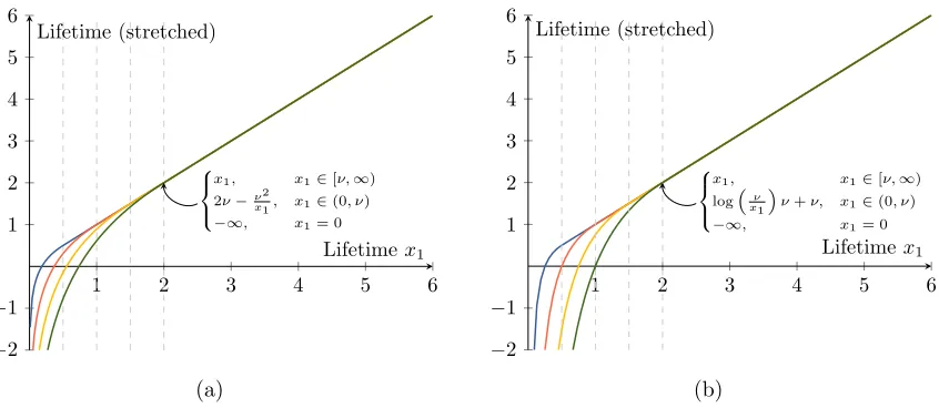
Figure 2: Stretching the lifetime axis of a birth-lifetime transformed (cf. Def.15) barcode via (a) the transform proposed in Eq. (10) and (b) the log-stretching previously proposed byHofer et al.(2017a). Different values ofν are marked by dashed lines. While, the differences appear subtle, the stretching as in (a) allows to guarantee Lipschitz continuity ofall proposed structure elements (Section5.4), whereas (b) only works for exponential structure elements (Section5.4.1).
results in a notable simplification. We summarize this step in the following definition of a
birth-lifetime coordinate transform, similar to (Adams et al.,2017).
Definition 15 (Birth-lifetime coordinate transform) We define
ρ: Ω∪∆→R×[0,∞) (b, d)7→(b, d−b) .
as the birth-lifetime coordinate transform of a barcode.
The transform ρ enables representing barcodes as multi sets over the upper half-plane of R2.
5.2. Rationally stretched birth-lifetime coordinates
Second, we introduce a transform, τ, on top ofρ, such that we can represent barcodes as multi sets overR×(R∪ {−∞}). We use the convention that for some functionf :R→R,
f(−∞) = limx→−∞f(x), if the limit exists and it is not defined otherwise.
The advantage of splitting the structure element into a composition of ρ,τ andtθ is that
is allows to use parametrized functionalstθ defined onR×Ras a starting point and then
require thattθ vanishes onR× {−∞}=τ◦ρ(∆). For example, most continuous probability
density functions are subject to this constraint. As a consequence, we can use the rich pool of such functions to find possible candidates fort.
Definition 16 (Rationally stretched birth-lifetime transform) For 0< ν, we define the birth-lifetime transform
by
τν((x0, x1)) =
(x0, x1), x1 ∈[ν,∞), (x0,2ν−ν
2
x1), x1 ∈(0, ν),
(x0,−∞), x1 = 0 .
(10)
Note thatτν is continuous onR2 as
lim
x→νx=ν = limx→ν2ν−
ν2 x .
As a consequence, we can define a parametrized functional, say
t: Θ→ {f :R×(R∪ {−∞})→R} θ7→tθ ,
on R×(R∪ {−∞}) such that
s=t◦τν◦ρ: Θ→ {f : Ω∪∆→R} θ7→sθ =tθ◦τν ◦ρ
is a structure element iff t (x0,−∞)
= 0. A visualization of the proposed birth-lifetime transform is shown in Figure2b, in comparison to the original (but limited) variant introduced inHofer et al.(2017a).
5.3. Lipschitz continuity
As we are especially interested in a stability preserving vectorization, we want to construct structure elements which are Lipschitz continuous, see Section 4. While the transform τν ◦ρ facilitates the selection of t, it also comes at a price. A closer examination reveals
that τν is not continuous on ∆ and hence not Lipschitz continuous. As a consequence,
Lipschitz continuity of some functionaltis not enough to guarantee thatt◦τν◦ρis Lipschitz
continuous. The core of the problem is that τν◦ρ diverges for (x0, x1)→(x0,0). In order to preserve Lipschitz continuity, a chosen functional t has to converge rapidly enough to dominate this divergence. In the following, we provide the essential argumentation to verify the Lipschitz condition fort◦τν ◦ρ. We start with two remarks to recall some properties of
Lipschitz continuous functions.
Remark 17 To show that a multivariate functionf :RN →R is Lipschitz continuous with respect tok·kq,1≤q ≤ ∞, it is sufficient that Lipschitz continuity with respect tok·kq holds
in each coordinate. The reason is that coordinate-wise Lipschitz continuity with respect tok·kq
leads to Lipschitz continuity with respect to k · k1 by taking the maximum of the
coordinate-wise Lipschitz constants. As all q-norms are equivalent, that is, ck · kq0 ≤ k · kq≤Ck · kq0
Our strategy to verify that a construction of the formt◦ρν◦τ is Lipschitz continuous will
be as follows: First, let ν >0 andt:R×R→Rbe Lipschitz continuous. Then, it suffices
to verify Lipschitz continuity of t◦τν onR×[0,∞), as ρ is trivially Lipschitz continuous. Second, for all following variants oft in Section 5.4, it will be clear that R×[ε,∞), ε >0
poses no problem and it remains to study the behavior of t◦τν onR×[0, ε). Now, as all
variants oft will also be Lipschitz continuous in the first coordinate,x0, only the second coordinate,x1, needs to be considered (Remark 17) and our strategy boils down to show
∂ ∂x1
t◦τν
< C ∈R on [0, ε) .
In all of the following cases, this will be equivalent to
lim
x→0
∂ ∂x1
t◦τν
(x)
< C ∈R ,
as the partial derivative of t◦τν will be continuous on (0, ε).
5.4. Structure elements
Next, we use the previous ideas to introduce (radial) structure elements which result in wq1 stable vectorizations. In particular, we start with a structure element based on the exponential function, analyze its properties, and then successively refine this element by switching to rational functions for better numerical stability and compatibility of the parameter gradients. Our main motivation is, to build structure elements that integrate well into a deep learning framework.
Remark 18 This section iteratively refines the structure element originally proposed by Hofer et al. (2017a), eventually resulting in the rational hat structure element of Section 5, Definition 23. We choose this type of presentation, as it elucidates certain design choices. However, those (intermediate) steps are not necessary to understand the final form of the refined version and may be skipped.
5.4.1. Exponential structure element(s)
Exponential functions have been previously used by Reininghaus et al. (2015), Kusano et al.(2016) and Adams et al.(2017) to weight points in barcodes. In (Reininghaus et al.,
2015), the exponential function arises as the solution of a heat-diffusion problem, whereas in (Kusano et al.,2016) this is motivated by the idea of embedding measures into a reproducing kernel Hilbert space. The crucial difference to these approaches is that our structure elements
are not at fixed locations (that is, one element per point of the particular barcode), but their locations and scales are adjustable.
Definition 19 (Exponential structure element) We set Θ =R2×R2 with
((µ0, µ1),(σ0, σ1)) = (µ, σ)∈Θand define texp : Θ
→ {f :R×(R∪ {−∞})→R+}
Figure 3: Illustration of anexponential structure element, centered atµ= (1,2).
with
texp(µ,σ):R×(R∪ {−∞})→R+
(x0, x1)7→e−(σ
2
0(µ0−x0)2+σ12(µ1−x1)2) . We call sexpµ,σ =texpµ,σ◦τν◦ρ an exponential structure element.
Note thatsexpµ,σ is well-defined, that is, it is a structure element in the sense of Definition9.
This is obvious, as
sexp
µ,σ(∆) =texpµ,σ ◦τν◦ρ(∆) =texpµ,σ ◦τν(R× {0}) =texpµ,σ(R× {−∞}) ={0}
holds by design. An illustration of an exponential structure element, centered at µ= (1,2) is shown in Figure 3. The following lemma establishes Lipschitz continuity of this element.
Lemma 20 sexp(µ,σ) is Lipschitz continuous with respect tok · kq on Ω∪∆.
Proof see Appendix B.2
With respect to the differentiability ofsexp(µ,σ), it is easy to see thattexp(µ,σ)(x) is differentiable in Θ for x ∈ R2. Therefore, so is sexp(µ,σ)(x) forx ∈ Ω∪∆. As the differential operator is
additive, it follows that the induced barcode mapping,P
x∈Ds
exp
(µ,σ)(x), is differentiable.
5.4.2. Rational structure element(s)
The second structure element is inspired by rational functions of the form (1 +x)−n. Our
main intention is to simplifysexp such that we circumvent the exponential dependency of the diagram points. This is desirable in terms of numerical stability.
Definition 21 (Rational structure element) We set Θ =R2×R2×[1,∞) with
((µ0, µ1),(σ0, σ1), α) = (µ, σ, α)∈Θ and define trat : Θ→ {f :
R×(R∪ {−∞})→R+}
(µ, σ)7→trat
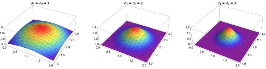
Figure 4: Illustration of arational structure element for σ0,1 = 1 and various choices ofα.
with
trat
(µ,σ,α):R×(R∪ {−∞})→R (x0, x1)7→
1
1 +|σ0| · |x0−µ0|+|σ1| · |x1−µ1|
α .
We call srat
(µ,σ,α)=t
rat
(µ,σ,α)◦τν◦ρ a rational structure element. Lemma 22 srat
(µ,σ,α) is Lipschitz continuous with respect tok · kq. Proof see Appendix B.3
An illustration of a rational structure element, centered at location µ= (1,2) is shown in Figure 4. Similar to the exponential structure element, we see thatsrat
(µ,σ,α) is differentiable inµi and σi fori= 1,2. However, in case of α, we have to introduce a slight restriction as
srat
(µ,σ,α) is only differentiable forα∈(1,∞). Regarding the partial derivatives, it is worth pointing out that
∂ ∂αs
rat
(µ,σ,α)(x) and ∂ ∂θs
rat
(µ,σ,α)(x) forθ∈ {σ0, σ1, µ0, µ1}
are scaled differently. More precisely, letf(µ, σ, x) denote the denominator, that is,
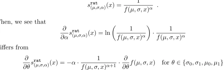
srat
(µ,σ,α)(x) = 1 f(µ, σ, x)α .
Then, we see that
∂ ∂αs
rat
(µ,σ,α)(x) = ln
1 f(µ, σ, x)α
· 1
f(µ, σ, x)α
differs from
∂ ∂θs
rat
(µ,σ,α)(x) =−α·
1
f(µ, σ, x)α+1 · ∂
∂θf(µ, σ, x) forθ∈ {σ0, σ1, µ0, µ1}
5.4.3. Rational hat structure element(s)
A closer look at srat reveals that the purpose of the parametersσ andα is to control the slope ofsrat
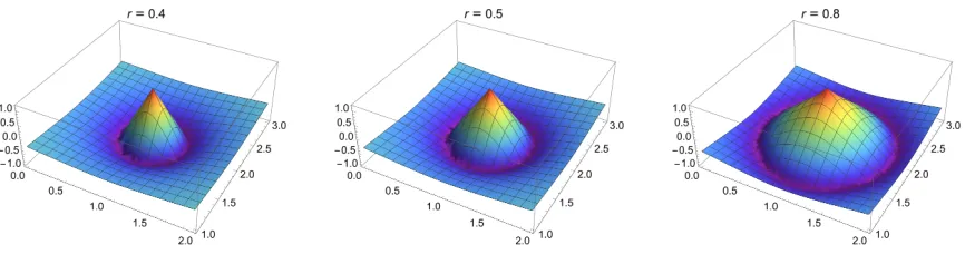
(µ,σ,α) aroundµ. To obtain a similar effect and to reduce the number of parameters, we gather this functionality into a single parameter r. We will see that this strategy yields a more balanced gradient scaling behavior. In detail, the idea is to use a uniformly scaled rational structure element and to subtract an antipode whose maximum is reached when the distance of a point to µis exactly r. This leads to the following definition.
Definition 23 (Rational hat structure element) We set Θ =R2×R×Nwith
((µ0, µ1), r, q) = (µ, r, q)∈Θ,x= (x0, x1)∈R×(R∪ {−∞}) and define
trat hat : Θ
→ {f :R×(R∪ {−∞})→R}
(µ, r, q)7→trat hat
(µ,r,q)
with
trat hat
(µ,r,q) :R×(R∪ {−∞})→R x7→ 1
1 +kx−µkq −
1
1 +| |r| − kx−µkq|
.
We call srat hat
(µ,σ,α) =trat hat(µ,σ,α) ◦τν◦ρ rational hat structure element.
To see that this structure element has the desired gradient behavior, lets consider the partial derivatives with respect to r and µi, that is,
∂ ∂r
trat hat (µ,r,q) (x)
(r) = sgn(|r| − kx−µkq|) (1 +| |r| − kx−µkq|)2 ·
sgn(r)
and
∂ ∂µi
trat hat (µ,r,q) (x)
(µi) = (−1)·
1
(1+kx−µkq)2 −
sgn(|r|−kx−µkq|) (1+| |r|−kx−µkq|)2
· ∂
∂µi(kx−µkq)(µi) .
We observe that both terms have similar order of growth in r andµi, respectively. However,
this comes at the price that we no longer have srat hat
(µ,σ,α)(µ) = 1. While this could be repaired by a multiplicative scaling factor
cr=
1 +|r| |r| , a closer look at
∂
∂rcr(r) =− sgn(r)
|r|2
reveals that this should be avoided, as it would lead to an undesirable quadratic dependency of the denominator with respect to r.
Lemma 24 trat hat
Figure 5: Illustration of a rational hat structure element fork·k2 and various choices ofr.
We omit the proof for brevity, but note that it is similar to the proof of Lemma 22. Furthermore,srat hat
(µ,σ,α)(D) is differentiable in its parameters. An illustration of this structure element, centered atµ= (1,2), for different parameter settings is shown in Figure5.
Overall, the advantages of srat hat over sexp and srat in terms of (1) the scaling of the derivatives and (2) its straightforward implementation, are particularly appealing for learning in the context of neural networks. Consequently, we use this element in all experiments that follow.
6. Experiments
We present a diverse set of experiments for supervised learning with different types of data objects. In particular, we show results for 2D/3D shape recognition and the classification of social network graphs, evaluated on standard benchmark data sets. Additionally, we present twoexploratory experiments for the problems of predicting the eigenvalue distribution of normalized graph Laplacian matrices and activity recognition from EEG signals. These experiments demonstrate the versatility and predictive power of persistent homology. Our goal is not to necessarily outperform approaches that are specifically tailored to a problem, but to demonstrate that persistent homology combined with deep learning delivers competitive performance in a very generic setup.
All experiments were implemented in PyTorch7, using DIPHA8 (Bauer et al., 2014) and
Perseus9 (Mischaikow and Nanda, 2013) for persistent homology computations. Source
code to fully reproduce the experiments is publicly-available10.
6.1. Network architecture
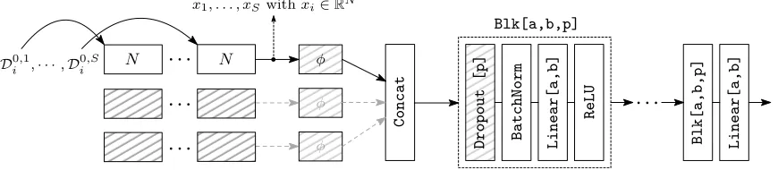
We focus on a generic neural network architecture, shown in Figure 6, that only needs to be slightly adjusted per experiment.
7.https://github.com/pytorch/pytorch
8.https://bitbucket.org/dipha/dipha
9.http://people.maths.ox.ac.uk/nanda/perseus
Blk[a,b,p]
Dropout
[p]
BatchNorm
Linear[a,b]
ReLU
Blk[a,b,p] Linear[a,b]
Concat
φ x1, . . . , xS withxi∈RN
N Di0,1,· · ·,D0i,S
φ
φ N
Figure 6: Illustration of our generic network architecture. Building blocks that are hatched are optional. One processing path (solid arrows) for handling S barcodes
Di0,1, . . . ,D
0,S
i fromone input objectoi are shown. In particular,D0i,j denotes the
S-th 0-dimensional barcode foroi. Handling homology groups of higher dimension
simply requires more input layers. The hyperparameterN denotes the number of structure elements per input layer.
For each filtration and homology dimension, we need one input layer. In Figure 6, an example with S 0-dimensional barcodes, Di0,1, . . . ,D
0,S
i , obtained from one input object oi,
is illustrated. Each input layer can have a varying number,N, of structure elements. We use the rational hat structure element (see Definition23) for the following reasons: First, we only need to learn two parameters per structure element, that is, µandr. Second, the gradients with respect to (µ, r) only differ by a linear term which we consider beneficial for learning. Third, commonly used building blocks of neural networks, for instance, batch normalization or rectified linear units (ReLU), expect both negative and positive inputs which is a property that only the rational hat element possesses. Overall, the output of one input layer is a vectorization in RN that is then concatenated with the output of
other input layers and fed into a multilayer perceptron (MLP). For optimization, we use stochastic gradient descent (SGD) with momentum and cross-entropy loss (if not mentioned otherwise). We additionally include a non-linearity φ:R→R(in our case φ= tanh) after
the input layer(s) to squash values in situations where points occur with high multiplicity; otherwise, φ = id. The parameter ν for the birth-lifetime transform of Definition 16 is fixed to 0.01 over all experiments11. We refer the reader to Table6 for a full specification of the network configurations. Regarding initialization of the structure elements, we run k-means++ (Arthur and Vassilvitskii,2007) clustering on all points from diagrams in the training portion of each dataset withk=N. TheN cluster centers are then used to initialize the position of the structure elements. The parameter r is set to 1/4 of the maximum lifetime of barcode elements in the training corpus. Different initializations ofr (within a reasonable range) only had a negligible impact on our results.
6.2. Baselines & Competitors
In all experiments onbenchmark data (Sections6.3 to6.5), we compare against two baselines.
First, we include a straightforward vectorization approach, followingBendich et al.(2016).
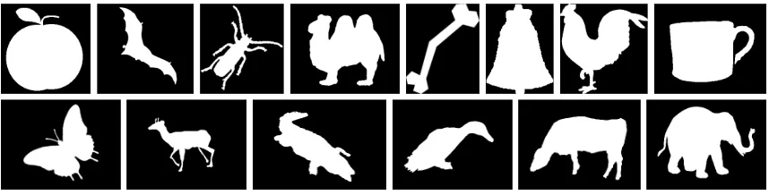
Figure 7: Some examples from the MPEG-7(top) and Animal(bottom) 2D shape datasets.
For each point (b, d) in a barcode D, we calculate its persistence d−b, sort the calculated persistences by magnitude from high to low and take the first N values. Hence, for each barcode, a vector of dimensionN (if|D \∆|< N, we pad with zero) is obtained. Then, a linear SVM (denoted as SVMlin) is trained withN determined by cross-validation on the training portion of each dataset (we denote this asBaseline in all experiments). Second, we include a baseline-like approach where the parametrization of the structure elements in our approach isonly initialized via k-means++ and then frozen during optimization. This allows to assess the impact of learning the parametrization of the structure elements.
We additionally compare against the persistence images approach from Adams et al. (2017) in two different variants. In its first incarnation, persistence images are computed on a 20×20 grid, vectorized (as originally suggested) and fed to a linear SVM. We use Gaussians centered at each point with the standard deviation determined via cross-validation (over σ∈ {0.1,0.5,1.0}). In its second incarnation, we compute persistence images for the three choices ofσ listed above and then use these images as amulti-channel input (that is, eachσ yields an input channel) to a convolutional neural network (NN) with one convolution layer (using 3×3 kernels and a stride of 2), followed by two fully-connected layers (interleaved with ReLUs). This setup is similar to Cang and Wei(2017) where barcodes are vectorized and fed to a 1D convolutional neural network. We use Adam (Kingma and Ba,2014) for optimization, train for 100 epochs with a batch size of 32, and use a learning rate of 0.01 (dropping to 0.001 after 50 epochs). This establishes a strong baseline and closely resembles our approach. For fair comparison, the number of (trainable) parameters in this network is comparable to the number of parameters in our architecture. We also found that including additional convolution layers did not further improve the results (in fact, unlike natural images, persistence images do not possess a compositional structure which would justify multiple convolution layers).
a0 a1 a2
a3 c0
c1
c2
c3
∆ ∆
(a0, a3)
(a1, a2)
(c0, c3)
(c1, c2)
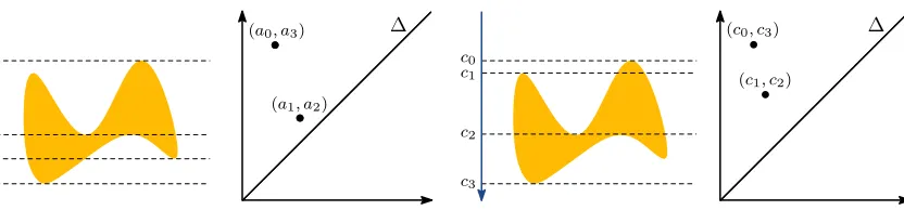
Figure 8: Height function filtration of a 2D shape from two directions, that is,ξ = (0,1) (left) and ξ0= (0,−1) (right), with their corresponding 0-dimensional barcodes (visualized as persistence diagrams).
grid) version of the PSS kernel feature map (or multiple feature maps, computed with varying PSS kernel scale parameter).
6.3. Recognition of 2D shapes
We first test our approach on two different datasets of 2D object shape recognition: (1) the Animaldataset, introduced byBai et al.(2009), which consists of 20 different animal classes, 100 samples each, and (2) theMPEG-7dataset which consists of 70 classes of different object/animal shapes, 20 samples each; see Latecki et al. (2000) for more details. For illustration, Figure 7 shows a selection of 2D object shapes from both datasets.
Filtration. The requirements to use persistent homology on 2D shapes are twofold: First, we need to assign a simplicial complex to each shape;second, we need to appropriately filter the complex. While, in principle, we could analyze contour features, such as curvature, and compute a sub level set filtration, such a strategy requires substantial preprocessing of the discrete data (for example, smoothing). Instead, we choose to work with the raw pixel data and leverage the persistent homology transform, introduced by Turner et al.
(2014b). The filtration in that case is based on sub level sets of theheight function, computed from multiple directions, illustrated in Figure 8. Practically, this means that we directly construct a simplicial complex from the binary image. We set K0 as the set of all pixels which are contained in the object. A 1-simplex [p0, p1] is in the 1-skeletonK1 iffp0 and p1 are 4–neighbors on the pixel grid. To filter the complex, we denote by β the barycenter of the object and by r the radius of its bounding circle around β. For [p]∈K0 andξ∈S1, the
filtration function is then given by
f([p]) = 1
r · hp−β, ξi ,
where h·,·i denotes the inner product in R2. The filtration is lifted to K1 by taking the maximum over the two vertices of each edge. Lettingξi denote 16 equidistantly distributed
directions in S1, starting from (1,0), we get a vector of barcodes (D0,j)16j=1. Here,D0,j is the barcode for 0-dimensional homology groups, obtained by filtration along ξj. As most
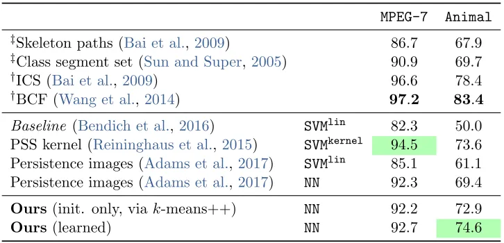
MPEG-7 Animal
‡Skeleton paths (Bai et al.,2009) 86.7 67.9 ‡Class segment set (Sun and Super,2005) 90.9 69.7 †ICS (Bai et al.,2009) 96.6 78.4 †BCF (Wang et al.,2014) 97.2 83.4
Baseline (Bendich et al.,2016) SVMlin 82.3 50.0
PSS kernel (Reininghaus et al.,2015) SVMkernel 94.5 73.6 Persistence images (Adams et al.,2017) SVMlin 85.1 61.1 Persistence images (Adams et al.,2017) NN 92.3 69.4
Ours (init. only, viak-means++) NN 92.2 72.9
Ours (learned) NN 92.7 74.6
Table 1: Average cross-validation accuracies (in %) on theAnimaland MPEG-7benchmark datasets, compared to the two best (†) and two worst (‡) results reported inWang et al. (2014), as well as different approaches that use persistent homology: our baselines from Section6.2 and the PSS kernel fromReininghaus et al. (2015).
all objects only have one connected component. For practical reasons, the death time of those essential points is set to the maximum filtration value of the corresponding direction. This has a natural geometric interpretation, as the persistence of these essential points is the diameter of the object along a direction.
Network configuration/training. We use the architecture of Figure 6 with φ= id and train with an initial learning rate of 0.01, a momentum of 0.9 and a batch size of 100 for 200 epochs. The learning rate is halved every 40-th epoch.
Results. Table1 lists the average cross-validation accuracies over 10 random 90/10 splits. Regarding approaches that also leverage information from persistent homology, we include the approaches of Section 6.2, as well as the PSS kernel from Reininghaus et al. (2015). For the PSS kernel, we train a kernel SVM using the averaged kernel matrices obtained for each filtration direction. In case of persistence images, multiple filtration directions simply increase the dimensionality of the vectorized input to the linear SVM, or the number of input channels in the neural network variant, respectively. When using SVMs, the cost parameter C is also determined via cross-validation on the training portion of each random split. Regarding non-topological strategies, we report the two best (†) and two worst (‡) results fromWang et al.(2014). While using topological signatures is below the top result on both datasets, we remark that no specific data preprocessing is required. This is in contrast to BCF or ICS which require contour extraction and are tailored to this type of data. Notably, in case of MPEG-7, the PSS kernel actually performs better than our approach. This can be
25 50 75 100 125 150 N
77.5 80.0 82.5 85.0 87.5 90.0 92.5
Avg. accuracy [%]
Learned (k-means) Learned (random) Frozen (k-means) Frozen (random)
0.0 0.2 0.4 0.6 0.8 0.00
0.25 0.50 0.75 1.00 1.25 1.50
(initialization) (learned)
0 50 100 150 200
Epochs 1.00
2.00 3.00 4.00
Loss
Train Test
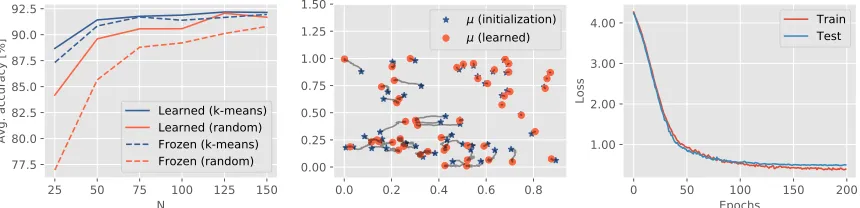
Figure 9: Left: Comparison, in terms of average cross-validation accuracy, of different initialization schemes, as a function of the number of structure elements,N, for two scenarios: (1) freezing the initial parameters and (2) learning the parametrization.
Middle: Example of the change in location of the rational hat structure elements during training (forN = 25) andrandom initialization. Right: Trainingvs. testing loss over the training epochs for the same setup.
combined with a convolutional neural network, perform better than simple vectorization combined with a linear SVM. Also, initialization viak-means++ exhibits good performance on MPEG-7, but is inferior to learning the parametrization of the input layer on theAnimal
dataset.
6.3.1. Effect of learning a task-specific vectorization
OnMPEG-7, we conduct a more detailed study on the impact oflearning the parametrization of the proposed input layer vs. different initialization schemes and no learning. This means that we compare against a parametrization that is only initialized, frozen during training, and only the classification part (that is, everything after the Concat layer in Figure 6) of the network is trained. Notably, by construction, even a random initialization outputs a vectorization that is 1-Wasserstein stable, however it is not optimized for the learning task. We experimented with different numbers of structure elementsN, as well as two initialization schemes: (1) random initialization and (2) initialization viak-means++ clustering (our default choice withk=N) of the points from all training diagrams. Figure9 (left) shows the average cross-validation accuracy onMPEG-7as a function of the number
Figure 10: 3D surface meshes for one example object from theSHREC14evaluation benchmark (Pickup, D. et al.,2014). Vertices x are colored by the heat-distributionh(x, t) at increasing values of t(fromleft to right). This relates to the scalar curvature ofx at scalet.
6.4. Recognition of 3D shapes
In this experiment, we consider the problem of 3D object recognition, based on features of the object’s surface mesh. We use the real watertight 3D surface meshes that are part of theSHREC14 benchmark and replicate the evaluation setup ofReininghaus et al. (2015). In
particular, this data set contains 400 watertight meshes, split into 40 classes with 10 samples per class. Each class represents one human in different poses.
Filtration. For each mesh, we compute the heat-kernel signature (HKS) ofSun et al.(2009) at 10 discrete time points ti, which captures the local heat distribution h(x, ti) at mesh
vertexx at scale ti. Figure 10illustrates the heat-distribution for one example object of
the SHREC14benchmark asti increases (fromleft toright). Similar to Section 6.5, we lift
the heat-distribution function to higher-dimensional simplices by taking the maximum over all faces and compute persistent homology of the sub level set filtration. Notably, in the kernel-based approach of Reininghaus et al.(2015), the optimal choice ofti is determined
via cross-validation and only diagrams for homology groups of dimension 0 are used12. In contrast, we use 0-and 1-dimensional homology and process the diagrams for eachti directly
via 20 parallel input layers (that is, 10 for dimension 0 and 10 for dimension 1). This is a natural choice and allows the network to focus on information relevant to the learning task.
Network configuration/training. We use the generic architecture of Figure6withφ= id and 20 input branches, that is, two input branches per HKS scale ti. The network is trained
for 300 epochs with a batch size of 20 and an initial learning rate of 0.5. The learning rate is halved every 20-th epoch.
Results. Table 2 lists cross-validation accuracies in comparison to specifically-tailored approaches, reported in Pickup, D. et al. (2014). We remark that results listed as APT,
supDLtrainRandR-BiHDM-s are obtained in a leave-one-out cross-validation setup using a
1-nearest neighbor classifier, due to the fact that Pickup, D. et al.(2014) assess retrieval