Variance-based Regularization with Convex Objectives
John Duchi [email protected]
Department of Statistics and Electrical Engineering Stanford University
Stanford, CA 94305, USA
Hongseok Namkoong [email protected]
Department of Management Science and Engineering Stanford University
Stanford, CA 94305, USA
Editor:Alexander Rakhlin
Abstract
We develop an approach to risk minimization and stochastic optimization that provides a convex surrogate for variance, allowing near-optimal and computationally efficient trading between approximation and estimation error. Our approach builds off of techniques for distributionally robust optimization and Owen’s empirical likelihood, and we provide a number of finite-sample and asymptotic results characterizing the theoretical performance of the estimator. In particular, we show that our procedure comes with certificates of optimality, achieving (in some scenarios) faster rates of convergence than empirical risk minimization by virtue of automatically balancing bias and variance. We give corroborating empirical evidence showing that in practice, the estimator indeed trades between variance and absolute performance on a training sample, improving out-of-sample (test) performance over standard empirical risk minimization for a number of classification problems.
Keywords: variance regularization, robust optimization, empirical likelihood
1. Introduction
We propose and study a new approach to risk minimization that automatically trades between bias—or approximation error—and variance—or estimation error. Let X be a sample space, P0 a distribution on X, and Θ a parameter space. For a loss function
`: Θ× X →R, consider the problem of findingθ∈Θ minimizing the risk
R(θ) :=E[`(θ, X)] =
Z
`(θ, x)dP(x) (1)
given a sample {X1, . . . , Xn} drawn i.i.d. according to the distribution P. Under appro-priate conditions on the loss `, parameter space Θ, and random variables X, a number of researchers (Bartlett et al., 2005, 2006; Boucheron et al., 2005; Koltchinskii, 2006) have shown results of the form that with high probability,
R(θ)≤ 1
n
n X
i=1
`(θ, Xi) +C1 r
Var(`(θ, X))
n +
C2
n for all θ∈Θ (2)
c
where C1 and C2 depend on the parameters of problem (1) and the desired confidence guarantee. Such bounds justify empirical risk minimization (ERM), which chooses θbn to minimize 1nPn
i=1`(θ, Xi) over θ ∈Θ. Further, these bounds showcase a tradeoff between bias and variance, where we identify the bias (or approximation error) with the empirical risk n1 Pn
i=1`(θ, Xi), while the variance arises from the second term in the bound.
Given bounds of the form above and heuristically considering the classical “bias-variance” tradeoff in estimation and statistical learning, it is natural to instead choose θ to directly minimize a quantity trading between approximation and estimation error, say of the form
1
n
n X
i=1
`(θ, Xi) +C
s Var
b
Pn(`(θ, X))
n , (3)
where Var
b
Pn denotes the empirical variance of its argument. Maurer and Pontil (2009)
considered precisely this idea, giving a number of guarantees on the convergence and good performance of such a procedure. Unfortunately, even when the loss`is convex inθ, the for-mulation (3) is in general non-convex, yielding computationally intractable problems, which has limited the applicability of procedures that minimize the variance-corrected empirical risk (3). In this paper, we develop an approach that provides a tractableconvex formulation whenever the loss ` is convex and very closely approximates the penalized risk (3). Our approach is based on Owen’s empirical likelihood (Owen, 2001) and ideas from distribu-tionally robust optimization (Ben-Tal et al., 2009; Bertsimas et al., 2014; Ben-Tal et al., 2015). Below, we give a number of theoretical guarantees and empirical evidence for its performance.
Before summarizing our contributions, we first describe our approach. Let φ:R+→R
be a convex function with φ(1) = 0. Then theφ-divergence between distributions P andQ
defined on a spaceX is
Dφ(P||Q) = Z
φ
dP dQ
dQ=
Z
X φ
p(x)
q(x)
q(x)dµ(x),
whereµ is any measure for which P, Qµ, andp= dPdµ,q = dQdµ. Throughout this paper, we use φ(t) = 12(t−1)2, which gives the χ2-divergence (Tsybakov, 2009). Given φ and a sampleX1, . . . , Xn, we define thelocal neighborhood of the empirical distribution with radius
ρ by
Pn:= n
distributionsP such thatDφ
P||Pbn
≤ ρ
n
o
,
wherePbndenotes the empirical distribution of the sample, and our choice ofφ(t) = 12(t−1)2 means thatPnconsists of discrete distributions supported on the sample{Xi}ni=1. We then define therobustly regularized risk
Rn(θ,Pn) := sup P∈PnEP
[`(θ, X)] = sup P
n
EP[`(θ, X)] :Dφ(P||Pbn)≤
ρ n
o
. (4)
As it is the supremum of a family of convex functions, the robust risk θ 7→ Rn(θ,Pn) is convex inθwhenever `is convex, no matter the value ofρ≥0. Given the robust empirical risk (4), our proposed estimation procedure is to choose a parameter θbnrob by minimizing
Let us now discuss a few of the properties of procedures minimizing the robust empirical risk (4). Our first main technical result, which we show in Section 2, is that for bounded loss functions, the robust riskRn(θ,Pn) is a good approximation to the variance-regularized quantity (3). That is,
Rn(θ,Pn) =EPbn[`(θ, X)] +
s 2ρVar
b
Pn(`(θ, X))
n +εn(θ), (5)
where εn(θ) ≤ 0 and is OP(1/n) uniformly in θ. We show specifically that whenever
`(θ, X) has suitably large variance, with high probability we have εn = 0. From variance expansions of the form (5) and empirical Bernstein inequality (2), we see that Rn(θ,Pn) is a O(1/n)-approximation to the population risk R(θ), in contrast to the cruder O(1/√n )-approximation that the empirical risk EPbn[`(θ;X)] provides. Based on this intuition that
the robustly regularized risk Rn(θ;Pn) is a tighter approximation to the population risk
R(θ), we show a number of finite-sample convergence guarantees for the estimator
b
θnrob ∈argmin θ∈Θ
sup
P n
EP[`(θ, X)] :Dφ
P||Pbn
≤ ρ
n
o
(6)
that are often tighter than those available for ERM (see Section 3). The above problem is a convex optimization problem when the original loss `(·;X) is convex and Θ is a convex set.
Based on the expansion (5), solutionsθbnrob of problem (6) enjoy automatic finite sample optimality certificates: forρ≥0, with probability at least 1−C1exp(−ρ) we have
R(θbnrob) =E[`(θbnrob;X)]≤Rn(θbnrob;Pn) +
C2ρ
n = infθ∈ΘRn(θ,Pn) +
C2ρ
n
where C1, C2 are constants (which we specify) that depend on the loss ` and domain Θ. That is, with high probability the robust solution has risk no worse than the optimal finite sample robust objective up to an O(ρ/n) error term. To guarantee a desired level of risk performance with probability 1−δ, we may specify the robustness penalty ρ=O(log1δ).
Secondly, we show that the procedure (6) allows us to automatically and near-optimally trade between approximation and estimation error (bias and variance), so that
R(θbnrob) =E[`(θbnrob;X)]≤ inf θ∈Θ
(
E[`(θ;X)] + 2
r 2ρ
nVar(`(θ;X))
) + Cρ
n (7)
Bounds that trade between risk and variance are known in a number of cases in the em-pirical risk minimization literature (Mammen and Tsybakov, 1999; Tsybakov, 2004; Bartlett et al., 2005; Boucheron et al., 2005; Bartlett et al., 2006; Boucheron et al., 2013; Koltchinskii, 2006), which is relevant when one wishes to achieve “fast rates” of convergence for statistical learning algorithms (that is, faster than theO(1/√n) guaranteed by a number of uniform convergence results (Bartlett and Mendelson, 2002; Boucheron et al., 2005, 2013)). In many cases, however, such tradeoffs require either conditions such as the Mammen and Tsybakov’s noise condition (Mammen and Tsybakov, 1999; Boucheron et al., 2005) or localization re-sults made possible by curvature conditions that relate the loss/risk and variance (Bartlett et al., 2006, 2005; Mendelson, 2014). The robust solutions (6) enjoy a different tradeoff between variance and risk than that in this literature, but essentially without conditions except compactness of Θ.
In proposing any new estimator, it is essential to understand the limits of the pro-posed procedure and identify situations in which its performance may be worse than ex-isting estimators. There are indeed situations in which minimizing the robust-regularized risk (4) yields some inefficiency (for example, in classical statistical estimation problems with correctly specified model). To understand limits of the inefficiency induced by using the distributionally-robustified estimator (6), in Section 4 we study explicit finite sample properties of the robust estimator for general stochastic optimization problems, and we also provide asymptotic normality results in classical problems. There are a number of situations, based on growth conditions on the population risk R, when convergence rates faster than 1/√n(or even 1/n) are attainable (see Shapiro et al. (2009, Chapter 5)). We show that under these conditions, the robust procedure (6) still enjoys (near-optimal) fast rates of convergence, similar to empirical risk minimization (also known as sample average approximation in the stochastic programming literature). Our study of asymptotics makes precise the asymptotic efficiency loss of the robust procedure over minimizing the standard (asymptotically optimal) empirical expectation: there is a bias term that scales as pρ/n
in the limiting distribution ofθbnrob, though its variance is optimal. o
We complement our theoretical results in Section 5, where we conclude by providing three experiments comparing empirical risk minimization strategies to robustly-regularized risk minimization (6). These results validate our theoretical predictions, showing that the robust solutions are a practical alternative to empirical risk minimization. In particular, we observe that the robust solutions outperform their ERM counterparts on “harder” instances with higher variance. In classification problems, for example, the robustly regularized es-timators exhibit an interesting tradeoff, where they improve performance on rare classes (where ERM usually sacrifices performance to improve the common cases—increasing vari-ance slightly) at minor cost in performvari-ance on common classes.
Related Work
5) for an overview in the case of classification, and Shapiro et al. (2009, Chapter 5.3) for more general stochastic optimization problems). Vapnik and Chervonenkis (1971, 1974) first provided such results in the context of {0,1}-valued losses for classification (see also (An-thony and Shawe-Taylor, 1993)), where the expectation of the loss always upper bounds its variance, so that if there exists a perfect classifier the convergence rates of empirical risk minimization procedures are O(1/n). Mammen and Tsybakov (Mammen and Tsybakov, 1999; Tsybakov, 2004) give low noise conditions for binary classification substantially gener-alizing these results, which yield a spectrum of fast rates. Under related conditions, Bartlett, Jordan, and McAuliffe (2006) show similar fast rates of convergence for convex risk mini-mization under appropriate curvature conditions on the loss. The robust procedure (6), on the other hand, is guaranteed to provide an at most O(1/n) over-estimate of the popula-tion risk and a small increase of its variance regularized populapopula-tion counterpart. It may be the case that the variance-regularized risk infθ{R(θ) +
p
Var(`(θ, X))/n} decreases to
R(θ?) more slowly than 1/n. As we note above and detail in Section 4, however, in stochas-tic optimization problems the variance-regularized approach (6) suffers limited degradation with respect to empirical risk minimization strategies, even under convexity and curvature properties that allow faster rates of convergence than those achievable in classical regimes, as detailed by (Shapiro et al., 2009, Chapter 5.3).
Most related to our work is that of Maurer and Pontil (2009), who propose directly regularizing empirical risk minimization by variance, providing guarantees similar to ours and giving a natural foundation off of which many of our results build. In their setting, however—as they carefully note—it is unclear how to actually solve the variance-regularized problem, as it is generally non-convex. Shivaswamy and Jebara (2010, 2011) build on this and develop an elegant approach for boosting binary classifiers based on a variance penalty applied to the exponential loss; as it is a boosting approach, their approach provides a coordinate-wise strategy for decreasing the loss, but it is not guaranteed to converge to a global minimizer and applies to classification-like problems. Our approach, handling general stochastic optimization problems, removes these obstructions.
The robust procedure (6) is based on distributionally robust optimization ideas that many researchers have developed (Ben-Tal et al., 2013; Bertsimas et al., 2014; Lam and Zhou, 2015), where the goal (as in robust optimization more broadly (Ben-Tal et al., 2009)) is to protect against all deviations from a nominal data model. In the optimization literature, there is substantial work on tractability of the problem (6), including that of Ben-Tal et al. (2013), who show that the dual of (4) often admits a standard form (such as a second-order cone problem) to which standard polynomial-time interior point methods can be applied. Namkoong and Duchi (2016) develop stochastic-gradient-like procedures for solving the problem (6), which efficiently provide low accuracy solutions (which are still sufficient for statistical tasks). Work on the statistical analysis of such procedures is nascent; Bertsimas, Gupta, and Kallus (2014) and Lam and Zhou (2015) provide confidence intervals for solution quality under various conditions, and Duchi et al. (2016) give asymptotics showing that the optimal robust risk Rn(θbnrob;Pn) is a calibrated upper confidence bound for infθ∈ΘE[`(θ;X)]. They and Gotoh et al. (2015) also provide a number of asymptotic
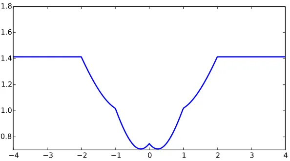
−4 −3 −2 −1 0 1 2 3 4 0.8
1.0 1.2 1.4 1.6 1.8
Figure 1. Plot ofθ7→p
Var(`(θ, X)) for`(θ;X) =|θ−X|whereX∼Uni({−2,−1,0,1,2}). The function is non-convex, with multiple local minima, inflection points, and does not grow asθ→ ±∞.
Notation We collect our notation here. We let B denote a unit norm ball in Rd, B =
{θ ∈Rd :kθk ≤ 1}, where dand k·kare generally clear from context. Given sets A ⊂Rd
and B ⊂ Rd, we let A+B = {a+b : a ∈ A, b ∈ B} denote Minkowski addition. For a convex function f, the subgradient set ∂f(x) of f at x is ∂f(x) = {g : f(y) ≥ f(x) +
g>(y −x) for all y}. For a function h : Rd → R, we let h∗ denote its Fenchel (convex)
conjugate, h∗(y) = supx{y>x−h(x)}. For sequences an, bn, we let an . bn denote that there is a numerical constantC <∞such thatan≤Cbnfor alln. For a sequence of random vectors X1, X2, . . ., we letXn
d
→X∞ denote thatXn converges in distribution toX∞. For
a nonegative sequence a1, a2, . . ., we say Xn =OP(an) if limc→∞supnP(kXnk ≥can) = 0, and we sayXn=oP(an) if limc→0lim supnP(kXnk ≥can) = 0.
2. Variance Expansion
We begin our study of the robust regularized empirical riskRn(θ,Pn) by showing that it is a good approximation to the empirical risk plus a variance term, that is, studying the variance expansion (5). Although the variance of the loss is in general non-convex (see Figure 1 for a simple example), the robust formulation (6) is a convex optimization problem for variance regularization whenever the loss function is convex (the supremum of convex functions is convex (Hiriart-Urruty and Lemar´echal, 1993, Prop. 2.1.2.)).
2.1. Variance expansion for a single variable
To gain intuition for the variance expansion that follows, we begin with a slightly simpler problem, which is to study the quadratically constrained linear maximization problem
maximize p
n X
i=1
pizi subject to p∈ Pn=
p∈Rn+: 1
2knp−1k 2
2≤ρ,h1, pi= 1
where z ∈ Rn is a vector. For simplicity, let s2
n = n1kzk 2
2−(z)2 = n1kz−zk 2
2 denote the empirical “variance” of the vector z, where z = n1 h1, zi is the mean value of z. Then by introducing the variableu=p−1
n1, the objective in problem (8) satisfieshp, zi=z+hu, zi=
z+hu, z−zi becausehu,1i= 0. Thus problem (8) is equivalent to solving
maximize u∈Rn
z+hu, z−zi subject to kuk22≤ 2ρ
n2, h1, ui= 0, u≥ −
1
n.
Notably, by the Cauchy-Schwarz inequality, we havehu, z−zi ≤√2ρkz−zk2/n=p2ρs2 n/n, and equality is attained if and only if
ui =
√
2ρ(zi−z)
nkz−zk2 =
√
2ρ(zi−z)
npns2
n
.
It is possible to choose such ui while satisfying the constraint ui≥ −1/n if and only if
min i∈[n]
√
2ρ(zi−z) p
ns2 n
≥ −1. (9)
Thus, if inequality (9) holds for the vector z—that is, there is enough variance in z—we have
sup p∈Pn
hp, zi=z+ r
2ρs2 n
n .
For losses `(θ, X) with enough variance relative to `(θ, Xi)−EPbn[`(θ, Xi)], that is, those
satisfying inequality (9), then, we have
Rn(θ,Pn) =EPbn[`(θ, X)] +
s 2ρVar
b
Pn(`(θ, X))
n .
A slight elaboration of this argument, coupled with the application of a few concentration inequalities, yields the next theorem. The theorem as stated applies only to bounded random variables, but in subsequent sections we relax this assumption by applying the characterization (9) of the exact expansion. As usual, we assume that φ(t) = 12(t−1)2 in our definition of the φ-divergence.
Theorem 1 Let Z be a random variable taking values in [0, M]. Let σ2 = Var(Z) and
s2n=EPbn[Z
2]−
EPbn[Z]
2 denote the population and sample variance of Z, respectively. Fix
ρ≥0. Then
r 2ρ
ns
2 n−
2M ρ n
!
+ ≤sup
P n
EP[Z] :Dφ(P||Pbn)≤
ρ n
o −E
b
Pn[Z]≤
r 2ρ
ns
2
n. (10)
Moreover, for n≥maxn2,Mσ22max{8σ,44}
o
, with probability at least 1−exp−3nσ2 5M2
sup P:Dφ(P||Pbn)≤nρ
EP[Z] =EPbn[Z] +
r 2ρ
ns
2
See Section A for the proof of Theorem 1.
Inequality (10) and the exact expansion (11) show that, at least for bounded loss func-tions `, the robustly regularized risk (4) is a natural (and convex) surrogate for empirical risk plus standard deviation of the loss, and the robust formulation approximates exact variance regularization with a convex penalty. In the sequel, we leverage this result to provide sharp guarantees for a number of stochastic risk minimization problems.
2.2. Uniform variance expansions
We now turn to a more uniform variant of Theorem 1, which depends on familiar notions of function complexity based on Rademacher averages. For a sample x1, . . . , xn and i.i.d. random signsεi∈ {−1,1}, independent of thexi, the empirical Rademacher complexity of the class F is
Rn(F) :=E "
sup f∈F
1
n
n X
i=1
εif(xi) #
.
The worst-case Rademacher complexity (Srebro et al., 2010) is
Rsupn (F) := sup x1,...,xn∈X
E
" sup f∈F
1
n
n X
i=1
εif(xi) #
.
For example, when F is a class of functions bounded by M with VC-subgraph dimension
d, we have the inequalitiesE[Rn(F)]≤Rsupn (F).M q
d
n. See van der Vaart and Wellner (1996, Chapter 2) and Bartlett and Mendelson (2002) for other bounds.
With this definition, we provide a result showing that the variance expansion (5) holds uniformly for all functions withenough variance.
Theorem 2 LetF be a collection of bounded functionsf :X →[0, M], andM ≤n. There exists a universal constant C such that if τ2>0 satisfies
τ2 ≥ 4ρM
2
n +C
Rsupn (F)2log3n+M 2
n (t+ log logn)
.
Then with probability at least 1−3e−t
sup P:Dφ(P||Pbn)≤ρn
EP[f(X)] =EPbn[f(X)] +
r 2ρ
nVarPbn(f(X)) (12)
for all f ∈ F such thatVar(f)≥τ2.
2.2.1. Linear and margin-based losses
Consider a standard margin-based classification problem (Bartlett and Mendelson, 2002), where we have data pairs (x, y) ∈ X × {−1,1}, and X ⊂ Rd. Let Θ ⊂ Rd be a norm
ball of radius r(Θ), Θ = {θ ∈ Rd | kθk ≤ r}, and let k·k
∗ be the associated dual norm,
assuming also that X ⊂ {x∈Rd| kxk
∗ ≤r(X)}. We may then consider the standard loss
minimization setting, where for some non-increasing and 1-Lipschitz loss ` :R → R+, we
have the risk
R(θ) :=E[`(Y hθ, Xi)],
so that `(yhx, θi) is the loss suffered by making prediction hθ, xi when the label is y. By taking the function classF={(x, y)7→`(yhx, θi)−`(0)|θ∈Θ}, in this case, an application of the Ledoux-Talagrand contraction inequality (Ledoux and Talagrand, 1991) implies for any y1, x1, . . . , yn, xn that
E
" sup θ∈Θ n X i=1
εi[`(yihθ, xii)−`(0)] # ≤E " sup θ∈Θ n X i=1
εihθ, xii #
≤r(Θ)E
" n X i=1
εixi ∗ # . (13)
Example 1 (Euclidean norms) In the above context, suppose that normk·kis the stan-dard `2 Euclidean norm so thatΘ is contained in an`2-ball of radius r(Θ), andX ⊂Rd in
an`2 ball of radius r(X). Then Jensen’s inequality and independence ofεi’s give the bound
E[k
n X
i=1
εixik]≤ v u u tE d X j=1 n X i=1
εixij !2
≤r(X)√n.
Then, inequality (13) and Theorem 1 imply that
sup P:Dφ(P||Pbn)≤nρ
EP[`(Y hθ, Xi)] =EPbn[`(Yhθ, Xi)] +
r 2ρ
nVarPbn(`(Y hθ, Xi))
for all θ satisfying
Var(`(Y hθ, Xi))≥ r(X) 2r(Θ)2
n
4ρ+Clog3n+Ct
,
with probability at least 1−e−t.
Example 2 (High-dimensional problems) In high dimensional problems, the Euclidean scaling of Example 1 may be problematic, so that using`1-constraints is preferred (B¨uhlmann and van de Geer, 2011). Thus, taking the normk·kin the preceding to be the`1 norm, so that Θ⊂ {θ∈ Rd | kθk1 ≤r1(Θ)} and k·k∗ =k·k∞, then E[k
Pn
i=1εixik∞] ≤r(X) p
nlog(2d), where r∞(X) denotes the `∞-radius of X ⊂ Rd. Thus, if we take the loss class F =
{`(hθ,·i)−`(0)|θ∈Θ}, we obtain
Rsupn (F). sup x1,...,xn∈X
r1(Θ)
n E " n X i=1
εixi ∞
#
≤r1(Θ)r∞(X)
r
log(2d)
n .
Then the exact variance expansion (12)holds with probability at least1−e−tuniformly over
θ satisfying Var(`(Y hθ, Xi))≥ r1(Θ)2r∞(X)2
n [4ρ+Clogd·log
2.2.2. Covering number guarantees
It is also possible to provide guarantees on the exact variance expansion using standard cov-ering numbers, though careful arguments based on Rademacher complexity can be tighter. We begin by recalling the appropriate notions from approximation theory. LetV be a vector space and V ⊂ V be any collection of vectors in V. Let k·kbe a (semi)norm onV. We say a collection v1, . . . , vN ⊂ V is an -cover of V if for each v ∈ V, there exists vi such that kv−vik ≤. The covering number of V with respect to k·kis then
N(V, ,k·k) := inf{N ∈N: there is an -cover ofV with respect to k·k}.
Now, letF be a collection of functions f :X →R, and define theL∞(X) norm onf by
kf −gkL∞(X):= sup x∈X
|f(x)−g(x)|.
We also relax our covering number requirements to empirical `∞-covering numbers as
fol-lows. Define F(x) = {(f(x1), . . . , f(xn)) : f ∈ F } for x ∈ Xn, and define the empirical
`∞-covering numbers
N∞(F, , n) = sup
x∈Xn
N(F(x), ,k·k∞),
which bound the number of `∞-balls of radius required to cover F(x). Note that we
always have N∞(F, , n) ≤ N(F, ,k·kL∞(X)) by definition. The classical Dudley entropy integral (Dudley, 1999; van der Vaart and Wellner, 1996) shows that, ifPndenotes the point masses onx1, . . . , xn and k·kL2(P
n) the empirical L
2-norm on functions f :X →[−M, M], then
E
" 1
nfsup∈F
n X
i=1
εif(xi) #
.inf δ≥0
δ+√1
n
Z M
δ q
logN(F, ,k·kL2(P
n))d
≤inf δ≥0
δ+√1
n
Z M
δ p
logN∞(F, , n)d
. (14)
Our main (essentially standard (van der Vaart and Wellner, 1996)) motivating example is that of Lipschitz loss functions for a parametric set Θ, as follows.
Example 3 Let Θ ⊂ Rd and assume that ` : Θ× X → [0, M] is L-Lipschitz in θ with respect to the `2-norm for all x ∈ X, meaning that |`(θ, x)−`(θ0, x)| ≤Lkθ−θ0k2. Then taking F = {`(θ,·) : θ ∈Θ}, any -covering {θ1, . . . , θN} of Θ in `2-norm guarantees that mini|`(θ, x)−`(θi, x)| ≤L for allθ, x. That is,
N(F, ,k·kL∞(X))≤N(Θ, /L,k·k2)≤
1 +diam(Θ)L
d
,
where diam(Θ) = supθ,θ0∈Θkθ−θ0k2. Thus `2-covering numbers of Θ control L∞-covering numbers of the family F, and we have by the entropy integral (14) that
Rsupn (F). r
d n
Z diam(Θ)L 0
r
logdiam(Θ)L
d.diam(Θ)L
r
d n.
3. Optimization by Minimizing the Robust Loss
Based on the precise variance expansions in the preceding section, it is natural to expect that the robust solution (6) automatically trades between approximation and estimation error. This intuition is accurate, and we show that the robustly regularized objective
Rn(θ;Pn) overestimates the population riskR(θ) by at mostO(1/n). By virtue of optimiz-ing this tighter approximation—as opposed to the usual O(1/√n)-approximation given by the empirical risk EPbn[`(θ;X)]—the robustly regularized solution (6) enjoys a number of
favorable finite-sample properties, which are not always comparable to those for empirical risk minimization (ERM).
In Section 3.1, we present two versions of our main result that depend on covering numbers and discuss their consequences, and we provide an example where the robustly regularized solution θbnrob achieves a tighter excess risk bound compared to those that a straightforward application of localized Rademacher complexities (Bartlett et al., 2005) show that the ERM solution θbnerm achieves. As evidenced by the substantial work on Rademacher- and Gaussian-complexity and symmetrization, in some instances covering-number-based arguments do not provide the sharpest scaling (Bartlett and Mendelson, 2002; Bartlett et al., 2005; Srebro et al., 2010); thus, in Section 3.2 we present a version of our main result that depends on localized Rademacher complexities, which can allow more refined uniform concentration bounds than covering numbers. We also provide a concrete (but admittedly somewhat contrived) example where our robustly regularized procedure (6) achievesR(θbnrob)−infθ∈ΘR(θ). lognn, while empirical risk minimization suffers R(θbnerm)− infθ∈ΘR(θ)& √1n, in Section 3.3. The robust “regularizer” has invariance properties other regularization procedures do not, and we mention these briefly in Section 3.4.
3.1. Covering arguments
Our first guarantee depends on the covering numbers of the function classF as we describe in Section 2.2.2. While we state our results abstractly, in the loss minimization setting we typically consider the function classF :={`(θ,·) :θ∈Θ}parameterized byθ. We have the following theorem, where as usual, we let F be a collection of functions f :X → [M0, M1] withM =M1−M0.
Theorem 3 Let n≥8M2/t, t≥log 12, >0, and ρ ≥9t. Then with probability at least 1−2(3N∞(F, ,2n) + 1)e−t,
E[f(X)]≤ sup
P:Dφ(P||Pbn)≤ρn
EP[f(X)] + 11
3
M ρ
n + 2 + 4
r 2t
n
!
(15)
for all f ∈ F. Defining the empirical minimizer
b
f ∈argmin f∈F
sup
P n
EP[f(X)] :Dφ(P||Pbn)≤
ρ n
o
we have with the same probability that
E[fb(X)]≤ inf f∈F
(
E[f] + 2
r 2ρ
nVar(f)
)
+19M ρ
3n + 2 + 4
r 2t
n
!
See Section C for a proof of the theorem. Because uniform L∞-covering numbers upper bound empiricalL∞-covering numbers, it is immediate that coveringFink·kL∞(X)provides an identical result.
3.1.1. Covering bounds: corollaries
We turn to a number of corollaries that expand on Theorem 3 to investigate its consequences. Our first corollary shows that Theorem 3 applies to standard Vapnik-Chervonenkis (VC) classes. As VC dimension is preserved through composition, this result also extends to the procedure (6) in typical empirical risk minimization scenarios.
Corollary 4 In addition to the conditions of Theorem 3, let F have finite VC-dimension VC(F). Then for a numerical constantc <∞, the bounds (15)and (16)hold with probability at least
1− cVC(F)
16M ne
VC(F)−1 + 2
!
e−t.
Proof LetkfkL1(Q):=
R
|f(x)|dQ(x) denote the L1-norm onF for the probability distri-bution Q. Then by Theorem 2.6.7 of van der Vaart and Wellner (1996), we have
sup Q
N(F, ,k·kL1(Q))≤cVC(F)
8M e
VC(F)−1
for a numerical constant c. Because kxk∞ ≤ kxk1, taking Q to be uniform on x ∈ X2n yieldsN(F(x), ,k·k∞)≤N(F,2n ,k·kL1(Q)). The result is immediate.
Next, we focus more explicitly on the estimator bθnrob defined by minimizing the robust regularized risk (6). Let us assume that Θ⊂Rd, and that we have a typical linear modeling situation, where a loss h is applied to an inner product, that is, `(θ, x) =h(θ>x). In this case, by making the substitution that the classF ={`(θ,·) :θ∈Θ}in Corollary 4, we have
VC(F)≤d, and we obtain the following corollary. In the corollary, recall the definition (1) of the population riskR(θ) =E[`(θ, X)], and the uncertainty setPn={P :Dφ(P||Pbn)≤ ρn}, and that Rn(θ,Pn) = supP∈PnEP[`(θ, X)]. By setting =M/n in Corollary 4, we obtain the following result.
Corollary 5 Let the conditions of the previous paragraph hold and letbθnrob ∈argminθ∈ΘRn(θ,Pn).
Assume also that `(θ, x)∈[0, M]for all θ∈Θ, x∈ X. Then if n≥ρ≥9 log 12,
R(θbnrob)≤Rn(θbnrob,Pn) + 11M ρ
3n +
2M n
1 +
r
ρ n
≤ inf
θ∈Θ (
R(θ) + 2 r
2ρ
nVar(`(θ;X))
)
+11M ρ
n
with probability at least 1 −2 exp(c1dlogn−c2ρ), where ci are universal constants with
c2 ≥1/9.
forδ >0, we define
ρ= log2
δ +dlog(2nDL). (17)
Settingt=ρand= n1 in Theorem 3 and assuming thatδ.1/n,D.nk andL.nk for a numerical constantk, choosingδ = n1 we obtain that with probability at least 1−δ= 1−1/n,
E[`(θbnrob;X)] =R(θbnrob)≤ inf θ∈Θ
(
R(θ) +C
r
dVar(`(θ, X))
n logn
)
+CdLDlogn
n (18)
whereC is a numerical constant.
3.1.2. Examples and heuristic discussion
Unpacking Theorem 3, the first result (15) (and its Corollary 5) provides a high-probability guarantee that the true expectation E[fb] cannot be more than O(1/n) worse than its robustly-regularized empirical counterpart. The second result (16) (and inequality (18)) guarantees convergence of the empirical minimizer to a parameter with risk at mostO(logn/n) larger than the best possible variance-corrected risk.
To illustriate how variance regularization can yield tighter guarantees than empirical risk minimization by optimizing a O(1/n) upper bound on the risk, we now compare the second bound (16) with an analogous result for empirical risk minimization (ERM). We first give a heuristic version, making it more precise in a coming example. For the ERM solution
b
θnerm∈argminθ∈ΘEPbn[`(θ;X)], one common assumption is an upper bound of the variance
by the risk; for example, when the losses take values in [0, M], one has Var(`(θ, X)) ≤
M R(θ). In such cases, there is typically some complexity measure Compn associated with the class of functions being learned, and it is possible to achieve bounds of the form
R(bθnerm)≤R(θ?) +C r
CompnM R(θ?)
n +C
CompnM
n (19)
whereθ?∈argminθ∈ΘR(θ), a type of result common for bounded nonnegative losses (Boucheron et al., 2005; Vapnik and Chervonenkis, 1971; Vapnik, 1998). For example, for classes of functions of VC-dimension d, we typically have Compn.dlognd. In this caricature, when Var(`(θ?, X))M R(θ?) and ρ&Compn, the optimality guarantee (16) for variance regu-larization can be tighter than its ERM counterpart (19). This bound is certainly not always sharp, but yields minimax optimal rates in some cases.
Example 4 (Well-specified least-absolute-deviation regression) For the least-absolute-deviation (LAD) regression, we compare rates of convergence for the ERM solution given by the localized Rademacher complexity against those for the robust solution. LetZ = (X, Y)∈
Rd×R, where X ∈ {x ∈Rd | kxk2 ≤L}, and let D:= diam(Θ) be the `2-diameter of Θ. The LAD loss is `(θ; (x, y)) :=|y− hθ, xi |, where we assume that Y =hθ?, Xi+for some
θ? ∈Θ, and random noise ∈ [−B, B] independent of X. We then have the global bound
`(θ; (X, Y)) ≤ DL+B =: M. Suppose for simplicity that is uniform on [−B, B]; then
θ? = argminθ∈ΘR(θ) and R(θ?) =E[`(θ?;Z)] = 12B. In this case, Var (`(θ?;Z)) = B
2 12 ≤
1
2(DL+B)B =ME[`(θ
Using that the loss is 1-Lipschitz, the L∞ covering numbers for the set of functions F := {fθ(x, y) = | hθ, xi −y| | θ ∈ Θ} satisfy logN(F, ,k·kL∞(X)) . dlogDL , and so applying the bound (18)for the robustly regularized solutionθbnrob with=DL/n, we obtain
R(θbnrob)≤R(θ?) +C r
dlogn
n B
2+Cd(LD+B) logn
n
with probability at least1−1/n. On the other hand, even an “optimistic” (but naive) ERM bound, achieved by taking Compn.1 in the bound (19), yields
R(θbnerm)≤R(θ?) +C r
logn
n (BDL+B
2) +C(LD+B) logn
n
with probability at least1−1/n. We see that leading term for the robustly regularized solution
b
θnrob only depends on the noise-level B2 while the corresponding term for the ERM solution
b
θnerm depends on global information like the size of the parameter space D, and a uniform bound over covariatesL. For typical VC and other d-dimensional classes, the bound Compn
scales linearly in d(cf. (Bartlett et al., 2005, Corollary 3.7), in which case the bound (19) scales as R(θ?) +Cpd(BDL+B2) logn/n+O(logn/n), which is worse.
Example 5 (A hard median estimation problem) To give a bit more insight into the behavior of the robust estimator, consider the simple 1-dimensional median problem, where
`(θ;x) = |θ−x|, and assume that x ∈ {−B, B} with P(X = B) = 1+δ2 for some δ > 0,
so that θ? = argminR(θ) = B and R(θ?) = (1−δ)B. In this case, taking θ0 = 0 yields Var(`(θ;X)) = 0andR(θ0)−R(θ?) =δB. Forδsmall (on the order of1/
√
n), with constant probability the empirical risk minimizer isθbnerm =−B, yielding riskR(θbnerm)−R(θ?) = 2δB.
On the other hand, with high probability θbnrob ≥0 (because Var(`(θ0;X)) = 0 as `(0;X)≡
B), and so R(θbnrob)−R(θ?)≤δB. This gap is of course small, but it shows that the robust
solution is more conservative: it chooses θbnrob so that large losses (of scale 2B) are less
frequent.
When the population problem is “easy”, it is often possible to achieve faster rates of convergence than the usual O(1/√n) rate. The simplest scenario where this occurs is if the problem is realizable R(θ?) = 0, in which case θbnerm has excess risk of the order
O(logn/n); see the bound (19). The robustly regularized solution bθnrob enjoys the same faster rates of convergence under the more general condition that Var(`(θ?;X)) is small. As a concrete instance of this, let `(θ;X) ∈ [0, M] and assume that `(θ;X) satisfies the conditions of the first part of Example 3, and let the problem be realizable R(θ?) = 0. Since Var(`(θ;X))≤M R(θ), we have from the bounds (18) and (19) that
R(θbnerm)≤
CdDLlogn
n and R(θb
rob n )≤
CdDLlogn
n .
For example, Var(`(θ;X)) = 0 allows for the existence of someθ0∈Θ such that`(θ0;X)<
3.2. Localized Rademacher Complexity
A somewhat more sophisticated approach to concentration inequalities and generalization bounds is based on localization ideas, motivated by the fact that near the optimum of an empirical risk, the complexity of the function class may be smaller than over the entire (global) class (van der Vaart and Wellner, 1996; Bartlett et al., 2005). With this in mind, we now present a refined version of Theorem 3 that depends on localized Rademacher averages. The starting point for this approach is a notion of localized Rademacher complexity (we give a slightly less general notion than Bartlett et al. (2005), as it is sufficient for our derivations). For a function class F of functions f : X → R, the localized Rademacher complexity at levelr is
ERn
cf |f ∈ F, c∈[0,1],E[c2f2≤r] .
In addition, we require a few analytic notions, beginning withsub-root functions, where we recall (Bartlett et al., 2005) that a function ψ :R+ → R+ is sub-root if it is nonnegative, nondecreasing, andr 7→ψ(r)/√r is nonincreasing for allr >0. Any non-constant sub-root functionψ is continuous and has a unique positive fixed point r? =ψ(r?), where r ≥ψ(r) for allr≥r?. Lastly, we consider upper boundsψ
n:R+→R+on the localized Rademacher complexity satisfying
ψn(r)≥E[Rn({cf :f ∈ F, c∈[0,1],E[c2f2]≤r})], (20)
where ψn is sub-root. (The localized Rademacher complexity itself is sub-root.) Roots of
ψnplay a fundamental role in providing uniform convergence guarantees, and Bartlett et al. (2005) and Koltchinskii (2006) provide careful analyses of localized Rademacher complexi-ties, with typical results as follows. For a class of functionsf with range bounded by 1, for any root rn? of ψn, with probability at least 1−e−t we have
E[f]≤EPbn[f] +
1
ηEPbn[f] +C(1 +η)
r?n+ 1
n
+ t
n for all f ∈ F and η≥0.
As an example, when F is a bounded VC-class, we have r?n VC(F) log(n/n VC(F)) (Bartlett et al., 2005, Corollary 3.7).
With this motivation, we have the following theorem.
Theorem 6 For M ≥ 1, let F be a collection of functions f : X → [0, M], let ψn be a sub-root function bounding the localized complexity (20), and let r?n≥ψn(rn?). Let t > 0 be arbitrary and assume that ρ satisfies
ρ
n ≥8
45M
n
t+ log l
logn
t
m
+ 18rn?
. (21)
Then with probability at least 1−e−t,
E[f]≤ 1 + 2
r 2ρ
n
!
sup P:Dφ(P||Pbn)≤ρn
EP[f] + 13 + 4 r
2ρ n
!
M ρ
Additionally, iffbminimizessupP:D
φ(P||Pbn)≤ρ/nEP[f], then with probability at least1−3e −t,
E[fb]≤ 1 + 2 r
2ρ n
! inf
f∈F E[f] +
r 91ρ
45nVar(f)
!
+ 14 + 6 r
2ρ n
!
M(3ρ+t)
n . (23)
We provide the proof of Theorem 6 in Appendix D. It builds off of and parallels many of the techniques developed by Bartlett, Bousquet, and Mendelson (2005), but we require a bit of care to develop the precise variance bounds we provide.
Let us consider the additional q
ρ
n factors in Theorem 6 (as compared to Theorem 3). In general, these terms are negligible to the extent that the variance of f dominates the first moment of the function f—heuristically, in situations in which we expect penalizing the variance to improve performance. Let us make this more precise in a regime wherenis large. Letting f ∈ F, we see that we have the inequality
(1 +pρ/n)
E[f] +
r
ρ
nVar(f)
≤E[f] +C
r
ρ
nVar(f)
(for a constantC >1 +pρ/n) if and only if (C−1−pρ/n)2Var(f)≥E[f]2. Equivalently,
as n gets large, this occurs roughly when E[f2] ≥ C
2−2C+2
C2−2C+1E[f]2, which holds for large enoughC whenever Var(f)>0.
In some scenarios, we can obtain substantially tighter bounds by using localized Rademacher averages instead of the covering number arguments considered in Section 3.1. (Recall also the discussion following Theorem 2.) To illustriate this point, we consider the case whereF is a bounded subset of a reproducing kernel Hilbert space generated by some sufficiently nice kernel K; even for the Gaussian kernelK(x, z) = exp(−12kx−zk2), log covering numbers for such function spaces grow at least exponentially in the dimension (Zhou, 2003; K¨uhn, 2011).
Example 6 (Reproducing kernels and least-absolute-deviation regression) We now give an example using a non-parametric class of functionals in which covering number ar-guments do not apply, as the covering numbers of the associated classes are too large. Let H be a reproducing kernel Hilbert space (RKHS) with norm k·kH and associated kernel (representer of evaluation) K : X × X → R. Letting P be a distribution on X,
Mer-cer’s theorem (e.g. Cristianini and Shawe-Taylor, 2004) implies that the integral opera-tor TK : L2(X, P) → L2(X, P) defined by TK(f)(x) =
R
K(x, z)dP(z) is compact, and
K(x, x0) =P∞
j=1λjφj(x)φj(z) whereλj are the eigenvalues ofT in decreasing order and φj form an orthonormal decomposition of L2(X, P).
Consider now the least absolute deviation (LAD) loss function `(h;x, y) = |h(x)−y|, defined for h ∈ H, and let BH be the unit k·kH-ball of H. Assume additionally that the
model is well-specified, and thaty=h?(x) +ξfor some random variableξ withE[ξ |X] = 0, E[ξ2]≤σ2, and h? ∈BH. Let the function class
{`◦ H}≤r :=
(x, y)7→c`(h(x), y)|c∈[0,1], c2E[`(h(X), Y)2]≤r .
Based on inequality (20), we consider the localized complexity
Rn({`◦ H}≤r) =E
" 1
nh∈BH,csup∈[0,1] X
εic`(h(xi), yi)|E[`(h(X), Y)2]≤r/c2
#
We claim that
Rn({`◦ H}≤r). p r/n+ 1 n ∞ X j=1
min{λj, r}
1 2
. (24)
As this claim is not central to our development—but does show a slightly different localization result based on Gaussian comparison inequalities than available, for example, in Mendelson (2003)—we provide its proof in Appendix G.1.
Let us use inequality (24). To apply Theorem 3, we must find a bound on the fixed point of the localized complexity. To give this bound, we require some knowledge on the eigenvalues λj, for which there exists a body of work. For example (Mendelson, 2003), the Gaussian kernel K(x, x0) = exp(−12kx−x0k22) generates a class of smooth functions for which the eigenvalues λj decay exponentially, as λj . e−j
2
. Kernel operators underlying Sobolev spaces with different smoothness orders (Birman and Solomjak, 1967; Gu, 2002) typically have eigenvalues scaling asλj .j−2α for someα > 12. As a concrete example, the first-order Sobolev (min) kernel K(x, x0) = 1 + min{x, x0} generates an RKHS of Lipschitz functions with α= 1. In the former case of λj .e−j
2 , rn? =
√ logn n 1 n ∞ X j=1 min
e−j2,logn n 1 2 ≈ 1 n √ logn X j=1 √ logn n + 1 n Z ∞ √ logn
e−t2dt
1 2 . √ logn
n =r
? n.
In the latter case of polynomially decaying eigenvalues λj .j−2α, we have j−2α =r when
r−21α =j, so
∞
X
j=1
min{j−2α, r} ≈r2α2−α1 +
Z ∞
r−1/2α
t−2αdtr2α2α−1.
Solving for nr=r2α2−α1, we find the fixed point (r?
n) 2α−1
4α =r?
n √
n yields rn? =n−2α2α+1. Ignoring constants, the above analysis shows that in the case that the kernel eigenvalues scale as λj .e−j
2
, as soon as ρ&√lognwe have
E[`(h(X), Y)]≤(1+2
p
2ρ/n) EPbn[`(h(X), Y)] +
r 2ρ
nVarPbn(`(h(X), Y))
! +Cρ
n for allh∈BH
with high probability. In the case of polynomial eigenvalues, if bh minimizes the robust
empirical loss supP:D
φ(P||Pbn)≤ρ/nEP[`(h(X), Y)] andρn
1− 2α
2α+1, then
E
h
`(bh(X), Y) i
≤1 +Cn−2αα+1
inf h∈BH
E[`(h(X), Y)] +Cn−
α
2α+1pVar(`(h(X), Y))
+Cn−2α2α+1.
This rate of convergence holds without any assumptions on the smoothness of the distribution of the noise ξ.
3.3. Beating empirical risk minimization
performance degradation to show that the formulation (6) in general loses little over empir-ical risk minimization. For intuition in this section, consider the (admittedly contrived) set-ting in which we replace the loss`(θ, X) with`(θ, X)−`(θ?, X), whereθ?∈argminθ∈ΘR(θ). Then in this case, by takingθ=θ? in Corollary 5, we haveR(θbnrob)≤R(θ?) +O(1/n) with high probability. More broadly, we expect the robustly regularized approach to offer per-formance benefits in situations in which the empirical risk minimizer is highly sensitive to noise, say, because the losses are piecewise linear, and slight under- or over-estimates of slope may significantly degrade solution quality.
With this in mind, we construct a concrete 1-dimensional example—estimating the median of a discrete distribution supported on X = {−1,0,1}—in which the robustly regularized estimator has convergence rate logn/n, while empirical risk minimization is at best 1/√n. Define the loss `(θ;x) =|θ−x| − |x|, and for δ ∈(0,1) let the distributionP
be defined by
P(X= 1) = 1−δ
2 , P(X=−1) = 1−δ
2 , P(X= 0) =δ. (25)
Then for θ∈R, the risk of the loss is
R(θ) =δ|θ|+1−δ
2 |θ−1|+ 1−δ
2 |θ+ 1| −(1−δ).
By symmetry, it is clear thatθ?:= argminθR(θ) = 0, which satisfiesR(θ?) = 0. (Note also that `(θ, x) =`(θ, x)−`(θ?, x).) Without loss of generality, we assume that Θ = [−1,1] in this problem.
Now, consider a sample X1, . . . , Xn drawn i.i.d. from the distribution P, let Pbn denote its empirical distribution, and define the empirical risk minimizer
b
θnerm := argmin θ∈R
EPbn[`(θ, X)] = argmin
θ∈[−1,1]
EPbn[|θ−X|].
If too many of the observations satisfyXi= 1 or too many satisfyXi =−1, thenθbnermwill be either 1 or−1; for smallδ, such events become reasonably probable, as the following lemma makes precise. In the lemma, Φ(x) = √1
2π Rx
−∞e −12t2
dtdenotes the standard Gaussian CDF. (See Section G.2 for a proof.)
Lemma 7 Let the loss`(θ;x) =|θ−x| − |x|, δ∈[0,1], and X follow the distribution (25). Then R(bθnerm)−R(θ?)≥δ with probability at least
2Φ − r
nδ2 1−δ2
!
−(1−δ2)n2
r 8
πn.
On the other hand, we certainly have`(θ?;x) = 0 for allx∈ X, so that Var(`(θ?;X)) = 0. Now, consider the bound in Theorem 3. We see that logN({`(θ,·) :θ∈Θ}, ,k·kL∞(X))≤ 2 log1, and taking= n1, we have that ifθbnrob∈argminθ∈ΘRn(θ,Pn), then
R(θbnrob)≤R(θ?) + 15ρ
In particular, takingρ= 3 logn, we see that
R(θbnrob)≤R(θ?) +
45 logn
n with probability at least 1−
4
n.
The risk for the empirical risk minimizer, as Lemma 7 shows, may be substantially higher; taking δ = 1/√n we see that with probability at least 2Φ(−q n
n−1) − 2 √
2/√πen ≥ 2Φ(−q n
n−1)−n
−1 2,
R(θbnerm)≥R(θ?) +n−
1 2.
(For n ≥ 20, the probability of this event is ≥ .088.) For this (specially constructed) example, there is a gap of nearly n12 in order of convergence.
3.4. Invariance properties
The robust regularization (4) technique enjoys a number of invariance properties. Standard regularization techniques (such as `1- and `2-regularization), which generally regularize a parameter toward a particular point in the parameter space, do not. While we leave deeper discussion of these issues to future work, we make two observations, which apply when Θ =Rdis unconstrained. Throughout, we letθbnrob ∈argminθRn(θ,Pn) denote the robustly regularized empirical solution.
First, consider a location estimation problem in which we wish to estimate the minimizer of the expectation of a loss of the form `(θ, X) = h(θ−X), where h :Rd → R is convex
and symmetric about zero. Then the robust solution is by inspection shift invariant, as
`(θ+c, X+c) =`(θ, X) for any vectorc∈Rd. Concretely, in the example of the previous section,`1- or`2-regularization achieve better convergence guarantees than ERM does, but if we shift all datax7→x+c, then non-invariant regularization techniques lose efficiency (while the robust regularization technique does not). Second, we may consider a generalized linear modeling problem, in which data comes in pairs (x, y)∈ X × Y and`(θ,(x, y)) =h(y, θ>x) for a function h:Y ×R→Rthat is convex in its second argument. Thenθbnrob is invariant to invertible linear transformations, in the sense that for any invertibleA∈Rd×d,
argmin θ
n
sup P:Dφ(P||Pbn)≤ρn
EP[`(θ,(X, Y))] o
= argmin θ
n
sup P:Dφ(P||Pbn)≤nρ
EP[`(A−1θ,(AX, Y))] o
=θbnrob.
Our results in this section do not precisely apply as we require unbounded θ, however, the next section shows that localization approaches can address this.
4. Robust regularization cannot be too bad
respect to ERM, considering two scenarios. The first is in stochastic (convex) optimization problems, where we investigate the finite-sample convergence rates of the robust solution to the population optimal risk. We show that the robust solution θbnrob enjoys fast rates of convergence in cases in which the risk has substantial curvature—precisely as with empirical risk minimization. The second is to consider the asymptotics of the robust solution θbnrob, where we show that in classical statistical scenarios the robust solution is nearly efficient, though there is an asymptotic bias of order 1/√nthat scales with the confidence ρ.
4.1. Fast Rates
In cases in which the risk R has curvature, empirical risk minimization often enjoys faster rates of convergence (Boucheron et al., 2005; Shapiro et al., 2009). The robust solutionθbnrob similarly attains faster rates of convergence in such cases, even with approximate minimizers of Rn(θ,Pn). For the riskR and ≥0, let
S?:=
θ∈Θ :R(θ)≤ inf
θ?∈ΘR(θ
?) +
denote the -sub-optimal (solution) set, and similarly let
b
S? :=
θ∈Θ :Rn(θ,Pn)≤ inf
θ0∈ΘRn(θ
0,P
n) +
.
For a vectorθ∈Θ, letπS?(θ) = argminθ?∈S?kθ?−θk2 denote the Euclidean projection ofθ onto the setS?; this projection operator is very useful for showing faster rates of convergence in stochastic optimization (see Shapiro et al. (2009), whose techniques we closely follow). In the statement of the result, forA⊂Θ, we letRn(A) denote the Rademacher complexity of the localized process {x 7→ `(θ;x)−`(πS?(θ);x) :θ ∈ A}. We then have the following
result, whose proof we provide in Section E.
Theorem 8 Let Θ be convex and let `(·;x) be convex and L-Lipshitz in its first argument for all x∈ X. For constants λ >0,γ >1, andr >0, assume the risk R satisfies
R(θ)− inf
θ∈ΘR(θ)≥λdist(θ, S?)
γ for allθ such that dist(θ, S?)≤r. (26)
Let t >0. If 0≤≤ 1
2λr
γ satisfies
≥
28
γLγ
λ
1
γ−1 ρ
n
γ
2(γ−1)
and
2 ≥2E[Rn(S 2 ? )] +L
2
λ
1
γ r2t
n, (27)
thenP(Sb?⊂S?2)≥1−e−t,
Corollary 9 In addition to the conditions of Theorem 8, assume that S? ={θ?} is a single point and Θ⊂Rd. Then for any ≤ 12λrγ, we have P(Sb? ⊂S?2)≥1−e−t for
&
Lγ λ
γ−11
d
nlog
n
d+
t
n +
ρ n
2(γγ−1)
.
So long as ρ.dlognd, this rate of convergence is as good as that enjoyed by standard empirical risk minimization approaches (Shapiro et al., 2009, Ch. 5) under these types of growth conditions. The case that γ = 2 corresponds (roughly) to strong convexity, and in this case we get the approximate rate of convergence of Lλ2dlog
n d
n , the familiar rate of convergence under these conditions. Of course, if there is too much variance penalization (i.e. ρ is too large), then the rates of convergence may be slower.
Proof That S? is a singleton implies that S?2 ⊂ {θ | kθ−θ?k ≤ (2/λ) 1
γ}. Moreover, in
this case we also have that
EPbn[`(θ;X)−`(θ
?;X)]−
EPbn[`(θ 0
;X)−`(θ?;X)] ≤L
θ−θ0
,
so that an /L-cover of {θ | kθ−θ?k ≤ (2/λ)1γ} is an -cover of the function class F =
{f(x) =`(θ;x)−`(θ?;x)|θ∈S?2} ink·kL2(P
n) norm. Thus, the standard Dudley entropy
integral (Dudley, 1999; van der Vaart and Wellner, 1996) yields
E[Rn(S?2)]. 1 √
n
Z ∞
0 q
logN(F, δ,k·kL2(P
n))dδ
. √1
n
Z L(2/λ)
1
γ
0
r
dlogL
δdδ≤L
r
d n
2
λ
γ1 s 1 +1
γ log
λ
2Lγ
where we have used that R0ε q
logLδdδ ≤ ε
q
1 + logLε. Solving for in the localization inequality (27) then yields the corollary, showing that the specified choice of is sufficient for all the conditions (27) to hold.
4.2. Asymptotics
It is important to understand the precise limiting behavior of the robust estimator in addi-tion to its finite sample properties—this allows us to more precisely characterize when there may bedegradation relative to classical risk minimization strategies. With that in mind, in this section we provide asymptotic results for the robust solution (6) to better understand the consequences of penalizing the variance of the loss itself. In particular, we would like to understand efficiency losses relative to (say) maximum likelihood in situations in which maximum likelihood is efficient. Before stating the results, we make a few standard assump-tions on the riskR(θ), the loss `, and the moments of` and its derivatives. Concretely, we assume that
θ? := argmin θ
that is, the risk functional has strictly positive definite Hessian atθ?, which is thus unique. Additionally, we have the following smoothness assumptions on the loss function, which are satisfied by common loss functions, including the negative log-likelihood for any exponential family or generalized linear model (Lehmann and Casella, 1998). In the assumption, we let
Bdenote the `2-ball of radius 1 in Rd.
Assumption A For some >0, there exists a function L:X →R+ satisfying |`(θ, x)−`(θ0, x)| ≤L(x)θ−θ0
2 for θ, θ
0 ∈θ?+
B
and E[L(X)2] ≤ L(P) < ∞. Additionally, there is a function H such that the function
θ7→`(θ, x)has H(x)-Lipschitz continuous Hessian (with respect to the Frobenius norm) on
θ?+B, where E[H(X)2]<∞.
Then, recalling the robust estimator (6) as the minimizer of Rn(θ,Pn), we have the following theorem, which we prove in Section F.
Theorem 10 Let Assumption A hold, and let the sequence θbnrob be defined by bθnrob ∈ argminθRn(θ,Pn). Define
b(θ?) := Cov(∇θ`(θ
?, X), `(θ?, X))
p
Var(`(θ?, X)) and Σ(θ
?) = ∇2R(θ?)−1
Cov(∇`(θ?, X)) ∇2R(θ?)−1.
Then θbnrob a.s.
→ θ? and √
n(θbnrob−θ?) d →N
−p2ρ b(θ?),Σ(θ?)
The asymptotic variance Σ(θ?) in Theorem 10 is generally unimprovable, as made ap-parent by Le Cam’s local asymptotic normality theory and the H´ajek-Le Cam local minimax theorems (van der Vaart and Wellner, 1996). Thus, Theorem 10 shows that the robust reg-ularized estimator (6) has some efficiency loss, but it is only in the bias term. We explore this a bit more in the context of the risk ofθbnrob. LettingW ∼N(0,Σ(θ?)), as an immediate corollary to this theorem, the delta-method implies that
nhR(θbnrob)−R(θ?) i d
→ 1 2
p
2ρ b(θ?) +W
2
∇2R(θ?), (28)
where we recall that kxk2A = x>Ax. This follows from a Taylor expansion, because ∇R(θ?) = 0 and so R(θ)−R(θ?) = 12(θ−θ?)>∇2R(θ?)(θ−θ?) +o(kθ−θ?k2), or
n(R(θbnrob)−R(θ?)) =n
1 2(θb
rob n −θ?)
>∇2R(θ?)( b
θnrob−θ?) +o(kθbnrob−θ?k2)
= 1 2
√
n(θbnrob−θ?) >
∇2R(θ?) √
n(θbnrob−θ?)
+oP(1)
d → 1
2( p
2ρ b(θ?) +W)>∇2R(θ?)(p
2ρ b(θ?) +W)
The limiting random variable in expression (28) has expectation
1 2E[k
p
2ρb(θ?) +Wk2∇2R(θ?)] =ρb(θ?)>∇2R(θ?)b(θ?) +
1 2tr(∇
2R(θ?)−1Cov(`(θ?, X)),
while the classical empirical risk minimization procedure (standardM-estimation) (Lehmann and Casella, 1998; van der Vaart and Wellner, 1996) has limiting mean-squared error
1 2tr(∇
2R(θ?)−1Cov(`(θ?, X))). Thus there is an additionalρkb(θ?)k2
∇2R(θ?) penalty in the
asymptotic risk (at a rate of 1/n) for the robustly-regularized estimator. An inspection of the proof of Theorem 10 reveals thatb(θ?) =∇θp
Var(`(θ?, X)); if the variance of the loss is stable near θ?, so that moving to a parameter θ = θ? + ∆ for some small ∆ has little effect on the variance, then the standard loss terms dominate, and robust regularization has asymptotically little effect. On the other hand, highly unstable loss functions for which ∇θp
Var(`(θ?, X)) is large yield substantial bias.
We conclude our study of the asymptotics with a (to us) somewhat surprising example. Consider the classical linear regression setting in which y =x>θ?+ε, where ε∼N(0, σ2). Using the standard squared error loss`(θ,(x, y)) = 12(θ>x−y)2, we obtain that
∇`(θ?,(x, y)) = (x>θ?−y)x= (x>θ?−x>θ?−ε)x=−εx,
while `(θ?,(x, y)) = 12ε2. The covariance Cov(εX, ε2) =E[εX(ε2−σ2)] = 0 by symmetry
of the error distribution, and so—in the special classical case of correctly specified linear regression—the bias term b(θ?) = 0 for linear regression in Theorem 10. That is, the robustly regularized estimator (6) is asymptotically efficient.
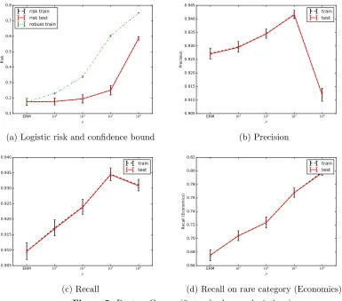
5. Experiments
We present three experiments in this section. The first is a small simulation example, which serves as a proof of concept allowing careful comparison of standard empirical risk minimization (ERM) strategies to our variance-regularized approach. The latter two are classification problems on real datasets; for both of these we compare performance of robust solution (6) to its ERM counterpart.
5.1. Minimizing the robust objective
As a first step, we give a brief description of our (essentially standard) method for solving the robust risk problem. Our work in this paper focuses mainly on the properties of the robust objective (4) and its minimizers (6), so we only briefly describe the algorithm we use; we leave developing faster and more accurate specialized methods to further work. To solve the robust problem, we use a gradient descent-based procedure, and we focus on the case in which the empirical sampled losses{`(θ, Xi)}ni=1 have non-zero variance for all parameters
θ∈Θ, which is the case for all of our experiments.
Recall the definition of the subdifferential∂f(θ) ={g∈Rd:f(θ0)≥f(θ)+hg, θ0−θi for allθ0},
which is simply the gradient for differentiable functionsf. A standard result in convex anal-ysis (Hiriart-Urruty and Lemar´echal, 1993, Theorem VI.4.4.2) is that if the vectorp∗ ∈Rn
achieving the supremum in the definition (4) of the robust risk is unique, then
∂θRn(θ,Pn) =∂θ sup
P∈PnEP
[`(θ;X)] = n X
i=1
p∗i∂θ`(θ;Xi),
where the final summation is the standard Minkowski sum of sets. As this maximizing vectorpis indeed unique whenever Var
b
Pn(`(θ;X))6= 0, we see that for all our problems, so
long as `is differentiable, so too isRn(θ,Pn) and
∇θRn(θ,Pn) = n X
i=1
p∗i∇θ`(θ;Xi) where p∗= argmax p∈Pn
n X
i=1
pi`(θ;Xi)
. (29)
In order to perform gradient descent on the risk Rn(θ,Pn), then, by equation (29) we require only the computation of the worst-case distribution p∗. By taking the dual of the maximization (29), this is an efficiently solvable convex problem; for completeness, we provide a procedure for this computation in Section H that requires time O(nlogn+ log1 logn) to compute an-accurate solution to the maximization (29). As all our examples have smooth objectives, we perform gradient descent on the robust risk Rn(·,Pn), with stepsizes chosen by a backtracking (Armijo) line search (Boyd and Vandenberghe, 2004, Chapter 9.2).
5.2. Simulation experiment
For our simulation experiment, we use a quadratic loss with linear perturbation. For
v, x ∈ Rd, define the loss `(θ;x) = 1
2kθ−vk 2 2 +x
>(θ −v). We set d = 50 and take X ∼ Uni({−B, B}d), varying B in the experiment. For concreteness, we let the domain Θ = {θ ∈ Rd :kθk2 ≤ r} and set v = 2√rd1, so that v ∈int Θ; we take r = 10. Notably,
standard regularization strategies, such as`1 or`2-regularization, pullθtoward 0, while the variance of `(θ;X) is minimized by θ =v (thus naturally advantaging the variance-based regularization we consider, asR(v) = infθR(θ) = 0). Moreover, asX is pure noise, this is an example where we expect variance regularization to be particularly useful. We choose
δ = .05 and set ρ as in Eq. (17) (using that ` is (3r+√dB)-Lipschitz) to obtain robust coverage with probability at least 1−δ. In our experiments, we obtained 100% coverage in the sense of (15), as the high probability bound is conservative.
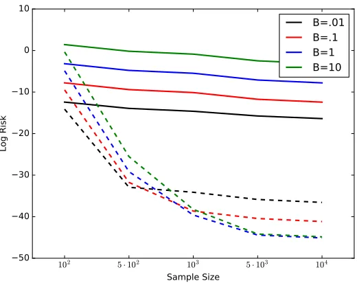
Figure 2 summarizes the results. The robust solutionθbnrob = argminθ∈ΘRn(θ,Pn) always outperforms the empirical risk minimizerbθnerm = argminθ∈ΘE
b
Pn[`(θ, X)] in terms of the true
riskE[`(θ, X)] = 21kθ−vk22. Each experiment consists of 1,200 independent replications for
102 5 · 102 103 5 · 103 104 Sample Size
−50 −40 −30 −20 −10 0 10
Lo
g R
isk
B=.01
B=.1
B=1
B=10
Figure 2. Simulation experiment. logE[R(bθnerm)] is the solid lines, in decreasing order from
B = 10 (top) to B =.01 (bottom). logE[R(bθnrob)] is the dashed line, in the same vertical ordering at sample sizen= 102.
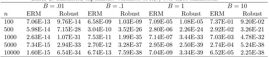
Table 1: Simulation experiment: Mean risks over 1,200 simulations
B =.01 B =.1 B = 1 B= 10
n R(θbnerm) R(θbnrob) R(θbnerm) R(θbnrob) R(θbnerm) R(θbnrob) R(bθnerm) R(θbnrob) 100 4.06E-06 7.42E-07 4.17E-04 7.65E-05 4.20E-02 7.64E-03 4.15E+00 7.12E-01 500 8.91E-07 5.01E-15 8.22E-05 1.63E-14 8.36E-03 2.19E-13 8.41E-01 8.21E-12 1000 4.47E-07 1.52E-15 4.02E-05 1.64E-17 4.20E-03 6.32E-18 4.19E-01 2.45E-17 5000 1.44E-07 2.68E-16 8.00E-06 2.74E-18 8.27E-04 5.09E-20 8.38E-02 6.55E-20 10000 7.64E-08 1.32E-16 4.02E-06 1.32E-18 4.13E-04 2.57E-20 4.18E-02 3.34E-20
5.3. Protease cleavage experiments
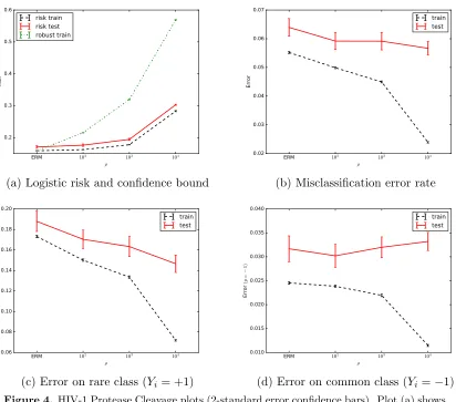
For our second experiment, we compare our robust regularization procedure to other regu-larizers using the HIV-1 protease cleavage dataset from the UCI ML-repository (Lichman, 2013). In this binary classification task, one is given a string of amino acids (a protein) and a featurized representation of the string of dimension d= 50960, and the goal is to predict whether the HIV-1 virus will cleave the amino acid sequence in its central position. We have a sample ofn= 6590 observations of this process, where the class labels are somewhat skewed: there are 1360 examples with label Y = +1 (HIV-1 cleaves) and 5230 examples withY =−1 (does not cleave).
We use the logistic loss`(θ; (x, y)) = log(1+exp(−yθ>x)). We compare the performance of different constraint sets Θ by taking
Θ = n
θ∈Rd:a1kθk1+a2kθk2 ≤r o