MRI Phase Mismapping Image Artifact Correction
Ashraf A. Abdallah1,*, Mawia A. Hassan2
1Medical Engineering Department, University of Science and Technology, Omdurman, Sudan 2Biomedical Engineering Department, Sudan University of Science and Technology, Khartoum, Sudan
Abstract
MRI machine one of the most significant diagnostic modalities. The only restriction that affects the MRI image is that imaging procedure take very long time comparing with CT scan and other diagnostic modalities, thus old patient, children and the illness people cannot stay without movement inside the magnet therefore artifact (phase mismaping artifact) will affect the MRI image and several miss analysis may occur especially in the neuroanatomical measurements. Many procedure has been use to solve this problem for example before during and after the MRI image reconstruction. In this study the effectiveness of a new retrospective motion correction technique has been applied and tested. Three different section MRI image (coronal, sagittal and axial) were used and given different correction results. That was by develop algorithm to correct the motion blur in the MRI image that corrupted by patient rigid motion. Wiener filter was used as the main restoration procedure by means of angle and length estimation of the motion blur. Motion blur angle and length were estimated using Hough transformer. The technique was applied and tested several time, it gave acceptable correction result in the sagittal image compare with the coronal one but the technique was result in the least motion blur correction in the axial image. Signal to noise ratio was calculated for every image to figure out the degree of the correction technique according to the different estimated angle and length. Signal to noise ratio values were to be through with correction result.Keywords
MRI, Motion estimation, Motion correction, S/N calculation, Motion artifacts (Phase Mismapping)1. Introduction
Magnetic resonance imaging (MRI) is an imaging technique used primarily in medical settings to produce high quality images of the inside of the human body. MRI is based on the principles of nuclear magnetic resonance (NMR), a spectroscopic technique used by scientists to obtain microscopic chemical and physical information about molecules. The technique was called magnetic resonance imaging rather than nuclear magnetic resonance imaging (NMRI) because of the negative connotations associated with the word nuclear. [1]. Artifacts caused by head and body motion pose a significant problem for the in vivo magnetic resonance imaging (MRI) of the human brain. Motion artifacts adversely affect the ability to accurately characterize the size, shape, and tissue properties of brain structures in both research subjects and clinical patients. In cognitive neuroscience applications, cross-sectional and longitudinal effects in neuroanatomical measurements are relatively small, making them easily obscured by distortions arising from patient and subject movement. Image quality is often degraded by motion artifacts, including image blurring and ghosting [1]. A number of techniques are employed to help in get rid of these problems: one is to prevent the motion
* Corresponding author:
[email protected] (Ashraf A. Abdallah) Published online at http://journal.sapub.org/ajbe
Copyright © 2016 Scientific & Academic Publishing. All Rights Reserved
occurring using sedation or physical restraints. Sedation involves risk [2] and also adds complication to the scan. Physically restraining patients is only partially effective. The objectives of this Thesis first is to develop algorithm to correct the motion blur in the MRI image that corrupted by patient rigid motion. Depend on the estimated angle and length and it’s important to develop an algorithm which can be estimate the angle and the length of motion blur MRI image finally determine the suitable angle and length which result in the maximum correction.
2. Correction Method
2.1. The Methodology Proceeds as Follows
First Appling Hough transformer function to the motion blurred image (Ifbl), to prepare motion angle estimation by building up the accumulator array.
Second Estimate the motion blur angle (THETA) using function that takes image as input and returns a collection of possible blur angles using step2 and other functions.
Third Estimate the length of the motion blur (LEN) which is the number of pixels by which the image is blurred the estimation depend on step2 beside other functions.
Forth Prepare the wiener filter algorithm using the estimation of angle and length of the motion blur and SNR as parameters.
wiener filter validation in motion blur correction.
2.2. Motion Blur Angle Estimation Algorithm
a) Performing Median Filter before restoring the blurred image and Display the input image.
b) Converting image from spatial domain to frequency domain.
c) Compute the log spectrum of F (u, v).
d) Convert the image to Cestrum (spectrum (IFT)) domain Compute the inverse Fourier transform of log spectrum.
e) Finding the edge map of the image in cepstral domain of step d.
f) Let theta min and the theta max be the minimum and maximum values of the motion blur angle.
g) Calling Hough transform to initialized the accumulator array.
h) Finding first maximum in the accumulator.
a) Performing Median Filter before restoring the blurred image and Display the input image.
b) Converting image from spatial domain to frequency domain.
c) Compute the log spectrum of F (u, v).
d) Convert the image to Cepstrum (spectrum (IFT)) domain Compute the inverse Fourier transform of log spectrum.
e) Rotate the cepstral by the estimated angle in the inverse direction.
f) Convert the 2-D matrix of step e to 1-D by taking the averages of columns.
g) Find the distance of first negative peak from the origin which is corresponding to motion length.
h) If Zero Crossing found then return it as the blur length i) If Zero Crossing not found then find the lowest peak
Calculating the blur length using Lowest Peak
Block Diagram 2. Illustrate motion Blur Angle Estimation Algorithm
transform was used in line detection, ten different expected angles and length of motion blur were estimated.
According to the different measured angles and lengths motion correction was applied by wiener filter ten times, the resulted images were treated by sharpening filters and SNR were measured for all corrected image in order to compare which estimated angle and length were result a better a
image has been illustrated following the coronal image figures, different angle and length for motion blur images has been estimated and accordingly different result was observed.
3.1. Coronal Sections
(a) (b) (c)
(d) (e) (f)
(j) (k)
Figure 1. (a) original image, (b,c,d,e,f,g,h,i,j,k) describe the motion blur correction images according to the following estimated angles and lengths as demonstrated in the table
The following table includes the estimated SNR for coronal corrected image in different angles and lengths comparing with the motion blurred image.
Table 1. Comparison between SNR of motion image and corrected image (coronal image)
Estimated angle (degree) & length(mm) Motion blurred image SNR corrected image SNR
(b) length: 11, angle: 112 -2.4619 -0.81093
(c) length: 11, angle: 99 -2.4619 -0.69318
(d) length: 5, angle: 173 -2.4619 -2.3216
(e) length: 13, angle: 179 -2.4619 -1.4268
(f) length: 7, angle: 2 -2.4619 -2.1138
(g) length: 7, angle: 16 -2.4619 -1.9739
(h) length: 4, angle: 62 -2.4619 -2.1776
(i) length: 9, angle: 131 -2.4619 -1.4626
(j) length: 7, angle: 145 -2.4619 -1.8852
(k) length: 4, angle: 124 -2.4619 -2.2321
Coronal sections discussion
By the visual inspection and consultation of radiologist and senior technologist comparing the original motion blurred image and motion corrected image. There is some anatomical structure were going to be diagnosable and clear more than before correction specially in angle 99° fig (5.2) and angle 112° fig (5.1) with the same length 11.
(a) (b) (c)
(d) (e) (f)
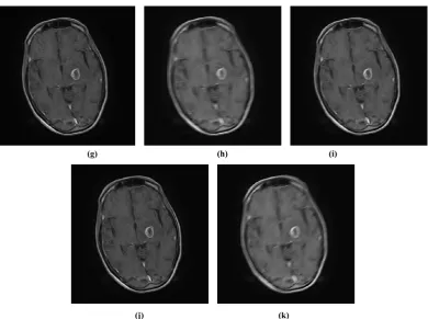
(g) (h) (i)
(j) (k)
The following table include the estimated SNR for sagittal corrected image in different angles and lengths comparing with the motion blurred image.
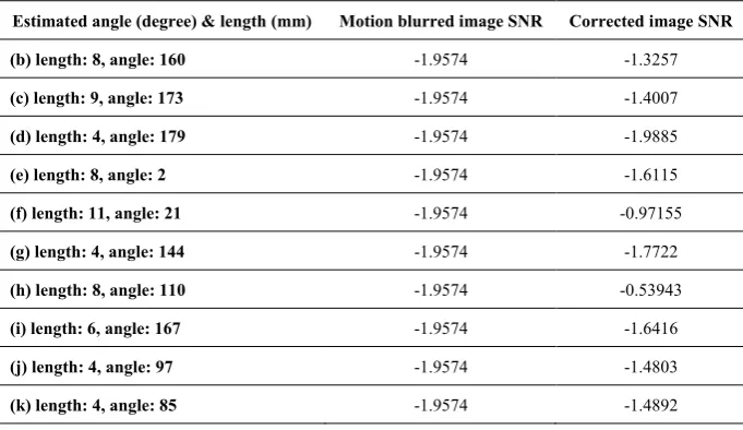
Table 2. Comparison between SNR of motion image and corrected image (sagittal image)
Estimated angle (degree) & length (mm) Motion blurred image SNR Corrected image SNR
(b) length: 8, angle: 160 -1.9574 -1.3257
(c) length: 9, angle: 173 -1.9574 -1.4007
(d) length: 4, angle: 179 -1.9574 -1.9885
(e) length: 8, angle: 2 -1.9574 -1.6115
(f) length: 11, angle: 21 -1.9574 -0.97155
(g) length: 4, angle: 144 -1.9574 -1.7722
(h) length: 8, angle: 110 -1.9574 -0.53943
(i) length: 6, angle: 167 -1.9574 -1.6416
(j) length: 4, angle: 97 -1.9574 -1.4803
(k) length: 4, angle: 85 -1.9574 -1.4892
Sagittal sections discussion
Also in the sagittal image the visual inspection and consultation of radiologist and senior technologist comparing the original motion blurred image and motion corrected image. There is some anatomical structure were going to be diagnosable and clear more than before correction specially in image (c) angle 173°, and image (e) with angle 2°, image (f) with angle 21°
and image (h) with angle 110°. The table (2) above contain the ten corrected image with their angles, lengths and SNR. Angle 21° image (f) and angle 110° image (h) had the maximum SNR value in the table which determine that it has the better motion blur correction even by the visual inspection the correction was clear and given clear result in the sagittal brain MRI image. For the remaining corrected image they gave some degrees of correction but different values of motion distortion was remained in the image and that is why the correction algorithm take different value of expected angles and lengths.
3.3. Axial Sections
(a) (b) (c)
(g) (h) (i)
(j) (k)
Figure 3. (a) original image, (b,c,d,e,f,g,h,i,j,k) describe the motion blur correction images according to the following estimated angles and lengths as demonstrated in the table
The following table include the estimated SNR for sagittal corrected image in different angles and lengths comparing with the motion blurred image.
Table 3. Comparison between SNR of motion image and corrected image (axial image)
Estimated angle (degree) & length (mm) Motion blurred image SNR corrected image SNR
(b) length: 10, angle: 172 -1.9394 -1.042
(c) length: 7, angle: 178 -1.9394 -1.5781
(d) length: 6, angle: 4 -1.9394 -1.6497
(e) length: 14, angle: 30 -1.9394 0.79873
(f), length: 7, angle: 110 -1.9394 -0.62628
(g) length: 4, angle: 162 -1.9394 -1.8385
(h) length: 14, angle: 11 -1.9394 -0.2526
(i) length: 6, angle: 23 -1.9394 -1.3499
(j) length: 3, angle: 145 -1.9394 -1.9133
(k) length: 7, angle: 116 -1.9394 -0.64491
Axial sections discussion
Finally in the axial corrupted image also by visual inspection and consultation of radiologist and senior technologist comparing the original motion blurred image and motion corrected image. There is some anatomical structure were going to be diagnosable and clear more than before correction specially in image (b) angle 172°, and image (c) with angle 178°, fig (5.15). The table (3) above contain the ten corrected image with their angles, lengths and SNR. For the remaining corrected image they gave some
degrees of correction but different values of motion distortion was remained in the image and that is why the correction algorithm take different value of expected angles and lengths.
4. Conclusions
Wiener filter was taken as the main algorithm in the correction procedure. According to ten different angles and lengths estimated before starting the correcting procedure. The correction algorithm achieved the best results which lead to clear appearance in anatomical brain feature and remove the motion blur which can obscure very important details. Although the corrected image by wiener filter gave a best result, it suffering some degree of unsharpeness, application of sharpening filter was needed and it gave better results. Motion blur in sagittal image result in highly degree of correction by the algorithm in the research. Since more than five images according to the different degree of angle and length estimation was totally corrected.
REFERENCES
[1] Google Internet, “General views”, Copy right J.P-Horn. [2] Liang Z-P, Lauterbur PC,” Principles of magnetic resonance
imaging: a signal processing perspective”, New York, Vol.4, No.16, 2000.
[3] Mohamed Abdullah, A., “the working principle of MRI lecture/Class”, University of medical science and technology, Vol.3, NO.6, 2008.
[4] Rskhandpur, “Hand book of bio medical instrumentation”, second edition, http://books.google.com/books.
[5] Wikipedia, “Hardware of MRI”, http://en.wikipedia.org/wiki/mri.
[6] Perry sprawls, Jr, Ph.D., FACR, “Physical principles of medical Imaging”, printed in United State of America, Vol.54, No.5, 2008.
[7] Mohamed Abdullah, A, “Hardware of MRI”, University of medical science and technology, Vol.12, No.3, 2008. [8] Perry sprawls, Ph.D., FACR, FAAPM, “Magnetic resonance
imaging”, Department of radiology mory university, Vol.23, No.7, 2009.
[9] Mohamed Abdullah, A, “Artifact of MRI”, University of medical science and technology, Vol.55, No.11, 2008. [10] Atkinson D,” Magnetic Resonance Imaging II”, Magnetic
Resonance in Medicine, Vol.44, No.9, 2012.
[11] Matthias Schlogl,” Motion Correction in MRI”, Magnetic Resonance in Medicine, Vol.13, NO.5, 2013.
[12] Mark Jenkinson, Peter Bannister, “Improved Optimization for the Robust and Accurate Linear Registration and Motion Correction of Brain Images”, Elsevier Science (USA), Vol.17, No.10, 2002.
[13] Stefan Thesen, Oliver Heid,” Prospective Acquisition Correction for Head Motion with Image-based Tracking for Real-Time fMRI”, Computer methods in Biomechanics and Biomedical engineering,Vol.30, No.11, 2009.
[14] Timothy T. Brown, Joshua M. Kuperman, “Prospective motion correction of high-resolution magnetic resonance imaging data in children”, journal homepage: www.elsevier.com/locate/ynimg, Vol.53, No.2, 2010.
[15] Gary H. Glover, Tie-Qiang Li, “Image-Based Method for Retrospective Correction of Physiological Motion Effects in fMRI: RETROICOR”, Magnetic Resonance in Medicine, Vol.44, No.8, 2000.
[16] Peter Kochunov, Jack L. Lancaster, “Retrospective Motion Correction Protocol for High-Resolution Anatomical MRI”, Human Brain Mapping, Vol.27, No.11, 2006.
[17] Alexander Loktyushin, Hannes Nickisch, “Blind Retrospective Motion Correction of MR Images”, Medical Imaging, Vol.55, No.7, 2007.
[18] James G. Pipe, “Periodically Rotated Overlapping ParallEL Lines with Enhanced Reconstruction (PROPELLER) MRI; Application to Motion Correction”, Proceedings of the International Society for Magnetic Resonance in Medicine Sixth Scientific Meeting and Exhibition Sydney, V0l.22, NO.5, 2011.
[19] Belma Dogdas, Quanzheng Li, “Motion Correction with Propeller MRI: Application to Head Motion”, International Journal of Electrical, Electronics and Computer Systems, Vol.26, No.12, 2010.
[20] Julian Maclaren, Michael Herbst, “Prospective Motion Correction in Brain Imaging: A Review”, Suffix Indicating a Corporation, Vol.23, No.6, 2012.
[21] Shamik Tiwari, V. P. Shukla, “Review of Motion Blur Estimation Techniques”, Image and Graphics, Vol.1, No.4, 2013.
[22] R. C. Gonzalez and R. E. Woods, “Digital Image Processing”, Prentice Hall, Vol.33, No.4, 2007.