PhD Dissertation
International Doctoral School in Information and Communication Technology
DISI - University of Trento
M
ACHINE
L
EARNING FOR
T
RACT
S
EGMENTATION IN D
MRI
DATA
Nguyen Thien Bao
Advisor:
Prof. Paolo Avesani
Co-Advisor:
Dr. Emanuele Olivetti
Universit`a degli Studi di Trento
Abstract
to the vector of distances from prototypes. Second, an algorithm is proposed to find the correspondence/mapping between streamlines in tractographies among two different samples, without requiring any transformation as the traditional tractography registration usually does. In other words, we try to find a map-ping between the tractographies. Mapping is very useful for studying tractog-raphy data across subjects. Last but not least, by exploring the mapping in the context of dissimilarity representation, we also propose the algorithmic solution to build the common vectorial representation of streamlines across subject. The core of the proposed solution combines two state-of-the-art elements: first using the recently proposed tractography mapping approach to align the prototypes across subjects; then applying the dissimilarity representation to build the com-mon vectorial representation for streamline. Preliminary results of applying our methods in clinical use-cases show evidence that our proposed algorithm is greatly beneficial (in terms of time efficiency, easiness.etc.) for the study of white matter tractography in clinical applications.
Keywords
Machine Learning, Tract Segmentation, Brain Connectivity, dMRI Data, Neuro Imaging
Acknowledgements
I wish to express my sincere appreciation and thanks to my advisor professor Dr. Paolo Avesani, for the excellent guidance and advice dur-ing the entire course of my PhD. His wise academic advice and ideas have played an extremely important role in the work presented in this thesis. Without Prof. Paolo’s support, this thesis would not have been possible. I also would like to be indebted the help of my co-advisor Dr. Emanuele Olivetti. His research suggestions and encouragement have been endless source of inspiration and support for my work.
I am also grateful to professor Dr. Lauren O‘Donnell at Harvard Uni-versity, for being so welcoming during my stay in the United States. Your advice on both research as well as daily life have been priceless. I would furthermore like to thank Dr. Eleftherios Garyfallidis for all his patience when explaining the basics of dMRI data, tractography, etc, at my very early step to work in this field. His constant availability for questions both in general theory and detail techique has been a great support for finishing this dissertation.
A big thank you to Nivedita Agarwal, Neuroradiologist at S. Maria del Carmine Hospital, and Assistant Professor of Neuroradiology, School of Medicine, who helped me with designing and collecting the dMRI data sets used in this work.
I would like to thank my friends and colleagues in NiLab - in partic-ular, Dr. Sandro Vega Pons, and Dr. Vittorio Lacovella for their inspira-tions and discussions.
A special thank to ICT, Doctoral School and CiMec of Trento Univer-sity, especially two secretaries of ICT, for their assistance during the past three years I stay in Italy.
My great acknowledgement to my master Ching Hai, for her
Finally, I would like to thank my family for their everlasting love and support. I want to give this dissertation as a present to my Father who always looks after my steps in life.
Nguyen Thien Bao Trento, 20 Feb. 2016
Publications
[1] Emanuele Olivetti,Thien B. Nguyen, and Eleftherios Garyfallidis. The approximation of the dissimilarity projection. The 2nd IEEE Interna-tional Workshop on Pattern Recognition in NeuroImaging, 0:8588, 2012. [2] Emanuele Olivetti, Thien B. Nguyen, and Paolo Avesani. Fast Clustering for Interactive Tractography Segmentation. The 3rd IEEE Inter-national Workshop on Pattern Recognition in NeuroImaging, 2013.
[3]Thien B. Nguyen, Emanuele Olivetti, and Paolo Avesani. Multiple-Scale visualization of large data based on hierarchical clustering. International Journal of Computer and Electrical Engineering, 6(2):7782, 2014.
[4]Thien B. Nguyen, Emanuele Olivetti, and Paolo Avesani. Mapping Tractography Across Subjects. NIPS Workshop on Machine Learning and Interpretation in Neuroimaging, MLINI 2014.
[5] Diana Porro-Munoz, Emanuele Olivetti, Nusrat Sharmin, Thien Bao Nguyen, Eleftherios Garyfallidis, and Paolo Avesani. Tractome: A Visual Data Mining Too for Brain Connectivity Analysis. International Jour-nal of Data Mining and Knowledge Discovery (DAMI), 2014.
[6] Paolo Avesani,Thien Bao Nguyen, Nivedita Agarwal, Mark Bromberg, Lubdha Shah, and Emanuele Olivetti. Tractography Mapping for Dissimi-larity Space Across Subjects. The 5th IEEE International Workshop on Pat-tern Recognition in NeuroImaging (PRNI 2015), June 10-12 2015, Stan-ford University, CA, USA.
Posters
[1] Eleftherios Garyfallidis, Stephan Gerhard, Paolo Avesani, Thien B. Nguyen, Vassilis Tsiaras, Ian Nimmo-Smith, and Emanuele Olivetti. A software application for real-time, clustering-based exploration of tractogra-phies. In 18th Annual Meeting of the Organization for Human Brain Mapping (OHBM), 2012.
In 20th Annual Meeting of the Organization for Human Brain Mapping (OHBM) 2014, pages 1858, June 2014.
[3] Paolo Avesani, Emanuele Olivetti, Thien Bao Nguyen, Nusrat Sharmin, and Nivedita Agarwal. White-Matter Alignment Across Subjects by Tractography Mapping. In 21th Annual Meeting of the Organization for Human Brain Mapping (HBM 2015).
Software
Tractome: A Visual Data Mining Tool for Brain Connectivity Analysis
http://tractome.org/
https://github.com/FBK-NILab/tractome
Contents
1 Introduction 1
1.1 The Context . . . 1
1.2 The Problem . . . 4
1.3 The Solution . . . 6
1.4 Innovative Aspects . . . 8
1.5 Structure of the Thesis . . . 9
2 State of the Art 13 2.1 Diffusion magnetic resonance imaging (dMRI) data and deterministic tractography . . . 14
2.1.1 From raw data to NIfTI format . . . 14
2.1.2 Reconstruction . . . 16
2.1.3 Tracking . . . 18
2.2 Tractography segmentation . . . 21
2.3 Tractography registration . . . 26
2.4 Notation . . . 32
3 Dissimilarity Representation for Tractography 35 3.1 Introduction . . . 36
3.2 Methods . . . 37
3.2.1 The dissimilarity projection . . . 38
3.2.2 A measure of approximation . . . 38
3.3.1 Simulated data . . . 42
3.3.2 Tractography data . . . 43
3.3.3 Dissimilarity for fast clustering tractography . . . . 46
3.4 Discussion . . . 52
4 Mapping Tractography Across Subjects 55 4.1 Introduction . . . 56
4.2 Methods . . . 59
4.2.1 Tractography mapping . . . 59
4.2.2 Common vectorial representation across subjects . 63 4.3 Experiments . . . 65
4.3.1 Data and preprocessing . . . 66
4.3.2 Design experiments . . . 67
4.3.3 Results . . . 69
4.4 Discussion and Conclusion . . . 76
5 An Interactive Visual Tool for Tractography Segmentation 79 5.1 Introduction . . . 80
5.2 Basic Concepts and Related Works . . . 85
5.3 Tractome: A Visual Data Mining tool for tractography analysis . . . 87
5.3.1 Dissimilarity Representation . . . 90
5.3.2 Clustering . . . 94
5.3.3 Data Visualization and Interaction . . . 96
5.3.4 Limitations and potentialities of Tractome . . . 99
5.4 Software Architecture . . . 101
5.4.1 Presentation layer . . . 102
5.4.2 Application layer . . . 103
5.4.3 Data layer . . . 105
5.5 Experiments . . . 106
5.5.1 Dissimilarity Representation and Prototype Selec-tion . . . 108
5.5.2 Tractography exploration example . . . 111
5.5.3 Clustering analysis . . . 112
5.6 Case Study . . . 114
5.6.1 Corticospincal Tract segmentation for ALS disease analysis . . . 115
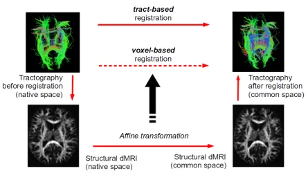
5.6.2 Comparison between voxel-based and tract-based registration . . . 118
5.7 Conclusions . . . 127
6 Conclusion 129 6.1 Summary . . . 129
6.2 Future works . . . 132
Bibliography 135
List of Tables
3.1 The average timings of the clustering algorithms using
mini-batch kmeans and dissimilarity representation . . . . 52
4.1 Data description: for each subject, the size of CST and
CST+ are reported, both as number of streamlines (the third and fourth column), and number of voxels (the last
column). . . 69
4.2 The result of mapping v.s three registration methods
(voxel-based FLIRT, tract-(voxel-based ODON [72], and tract-(voxel-based GARY [30]) on one subject . . . 73
4.3 The comparison of mapping with voxel-based and
tract-based registration method . . . 74
4.4 The performance of exploring the dissimilarity
represen-tation based on mapping . . . 76
4.5 The average of the performance when combining the
map-ping with dissimilarity for common vectorial representation 77
4.6 Average mean and standard deviation of true positive rate (TPR) and false discovery rate (FDR) for the four com-pared methods: FLIRT, ODON [72], GARY [30] and DMAP (dissimilarity + mapping). Results are aggregated in two
groups, according to the size of source and target tracts. . . 78
compute the clustering with k-means and MBKM is re-ported in the 3rd and 4th columns, respectively. The size (b) of the mini-batches for MBKM is in the 5th column. The time to compute the medoids from the centroids is in
the 6th column. . . 114 5.2 The average of the performance of the SVM CST classifier
over all subjects, in two atlas coordinate systems . . . 127
List of Figures
1.1 An example of streamlines, tractography, and tract . . . 2 1.2 The structural image of the brain with different type of
views . . . 3
2.1 An example of the DICOM image file . . . 15 2.2 Image acquired orthogonal to scanner bore . . . 16 2.3 An example of the dMRI data after doing brain extraction 18 2.4 Two approaches are usually used to simplify the visual
representation of 3D diffusion data . . . 19 2.5 Tracking from tensor direction information . . . 20 2.6 Two type of tracking algorithms: deterministic and
prob-abilistic algorithm. . . 21 2.7 Tractography registration: voxel based method and
tract-based method . . . 29 2.8 Streamline structural distances . . . 33
3.1 A set of 100 streamlines, i.e. an example of prototypes,
from a full tractography . . . 37 3.2 Example of points and prototype in 2D . . . 42 3.3 The dissimilarity projection of the simulated dataset and
prototypes . . . 43 3.4 The correlation distance between d and ∆dΠ in 2D with
random prototype selection policcy . . . 44
prototype selection policies and different numbers of
pro-totypes. . . 44 3.6 The correlation between of d and ∆dΠ over a 103
stream-lines tractography for different prototype selection policies. 46 3.7 The correlation between of d and ∆dΠ for a full
tractogra-phy of3×105 streamlines with random, and SFFprototype
selection policies. . . 47
4.1 The visualization of CST and CST extension from a whole
tractography . . . 70 4.2 Plots of the normalized loss (Lnorm = |CSTL
A|) as a function of number of iterations with simulated annealing in
map-ping . . . 71 4.3 The visualization of source, target and result of mapping
from source to target . . . 71 4.4 The visualization of the volume in voxel unit of CST
be-fore and after mapping . . . 72 4.5 Visualization of the result when the left CST of subject 204
is obtained from the left CST from subject 202: (A) FLIRT registration, (B) ODON [72], (C) GARY [30], (D) DMAP, dissimilarity and mapping. Blue color denotes the cor-rectly aligned streamlines, while the yellow color the
in-correct ones. . . 75
5.1 An example of streamlines and tractography . . . 81 5.2 The structural image of the brain with different type of
views . . . 81 5.3 Workflow of the Visual Data Mining tool for analysis of
tractography data. . . 88
5.4 Set of minimum distances (dotted lines) between each point of two streamlines sA and sB (solid lines). . . 92
5.5 Analyse First and Show Important. (A) Whole tractogra-phy. Streamlines are colored by following the Direction-ally Encoded Color convention [81]. (B) Visualization of
summary of the data by medoids of clusters. . . 97
5.6 Filtering. (A) Selected clusters (in white) (B) Only selected
clusters are shown. The rest were removed from the view. 98
5.7 Zooming. Streamlines belonging to the selected clusters are shown in the view, with a different line thickness and
colors. . . 98
5.8 The architecture of Tractome software in three-layer pattern.102
5.9 The graphic user interface (GUI) of Tractome software . . . 104
5.10 The list of functions of each class in Tractome software. . . 107
5.11 Average correlation between d and ∆dΠ across the differ-ent prototype selection policies and differdiffer-ent numbers of
prototypes. Each figure corresponds to a different subject. 110
5.12 The segmentation process. (A) Full tractography≈5×10⁵ streamlines; (B) Computation of 150 clusters (C) Selection of 11 clusters (in white); (D) ≈ 35000 streamlines corre-sponding to previous selection; (E) Computation of 50 clusters (F) Selection of 15 clusters; (G)≈ 9600streamlines corresponding to the previous selection; (H) Computation of 50 clusters (I) Selection of 15 clusters; (J)≈ 2000 stream-lines corresponding to the previous selection; (K) Compu-tation of 50 clusters (L) Selection of 25 clusters; (M) ≈650 streamlines corresponding to previous selection and
rep-resenting the segmented CST. . . 113
with487streamlines . . . 116 5.14 An example of the atlas after registration using tract-based
method . . . 121 5.15 The visualization of tracts from alll subjects in MNI space,
and in tract-based atlas . . . 122 5.16 An example of the input CST from controls and patients . 125 5.17 An example of the result of CST segmentation in one subject126
List of Algorithms
1 Mini-batch k-Means algorithm . . . 50 2 Common vectorial representation . . . 65
Chapter 1
Introduction
1.1
The Context
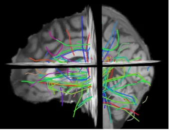
The brain, the central part of the nervous system, consists of the grey matter, known as cerebral cortex, and the white matter. Its core compo-nents are the neurons (nerve cells), that are in-charge of all the commu-nication and processing within the brain. Neurons are divided into three main parts: cell body, dendrites and axons. The grey matter is composed of dense concentrations of the cell bodies and dendrites of these neu-rons and all the processing of the brain takes place here. On the other hand, the white matter works as the brain’s connective cabling. It is composed of billions of myelinated axons that connect, i.e. transmit sig-nals between neurons in different regions of the brain [25]. The patterns and structures of these anatomical links between regions in the brain are known as anatomical connectivity [55] [17] of white matter. Anatomical connectivity can vary among people if, for example, they have mental disorders, neurologic or neuropsychiatric diseases. Therefore, research about the anatomical connectivity of the white matter hence becomes essential in neuroscience and is also the main focus of this work.
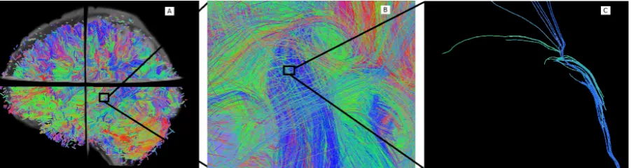
Figure 1.1: (A) Tractography overlaid with the structural image (only 10% of the streamlines are shown). The colour encodes the orientation of the mid-segment of every streamlines using a colour map based on [23]. (B) Amplifying an area of the tractography. (C) Small subset of streamlines.
The Context 3
Figure 1.2: The structural image of the brain with different type of views. The 2D views: (A) coronal, (B) sagittal, (C) axial
The exploration of tractography data sets has hence become very use-ful to neuroanatomists. Information like the shape of streamlines, their spatial location and the relation with each other, allows to identify and study the subsets of streamlines related to specific function(s). From there, it can be also determined if there is (or the status of) an ongoing neurodegenerative process.
ex-ploration i.e. shape recognition, spatial localization, quite difficult. See for example, in Figure 1.1.A, where only a 10% of the total amount of streamlines is shown, it is still difficult to visually understand the data.
1.2
The Problem
Recently, the literature about machine learning techniques to apply for analyzing and studying the white matter tractography is increasing. Al-though it has gained some encouraging results, but these results are still under the satisfactory of medical practitioners. In this work, we want improve the support of machine learning techniques for studying the white matter tractography. We want to help the medical practitioners to analyse the white matter tractography data more easily and more accu-rately based on machine learning techniques. The things that we want to investigate in this project are :
The Problem 5
supervised and unsupervised techniques get some encouraging re-sults, but they are below the expectation of medical practitioners. Unsupervised techniques usually work on the whole tractography while medical practitioner often focus on a specific tract. In the case of supervised learning, the lack of ground truth data makes the re-sults not good and need the refinement from experts. Although both supervised and unsupervised learning have gain some en-couraging results, but they are still under the satisfactory of medical practitioners. In this work, we try to assist the medical practition-ers to do the tract segmentation task more accurately, more easily in order to improve the quality of the segmentation.
• Vectorial representation for tractography streamline: Most of the machine learning and patern recognition techniques used for trac-tography analyses (such as supervised and unsupervised learning for tractography segmentation, clustering for tractography visulaiza-tion, ...) require the input to be from a vectorial space. This re-quirement contrasts with the intrinsic nature of the tractography because streamlines have different lengths and different number of points and for this reason they cannot be directly represented in a common vectorial space. This lack of the vectorial representation avoids the use of some of those algorithms and of computationally efficient implementations. In this thesis, we try to define a new rep-resentation for tractography streamline that can be fed to the most machine learning technigues.
techniques, for further analysis.
• A common vectorial representation for streamline across subjects:
Current neuroscientific analyses of white matter tractography data are limited to qualitative intra-subject comparisons. It is then quite difficult to use the information for direct inter-subject comparisons [37, 7]. Thus, when applying machine learning techniques for inter-subject tractography analyses, it leads to the need of defining a com-mon vectorial representation for tractography streamlines not only intra-subject but also across subjects.
1.3
The Solution
In this part, we shortly describe the solution for the problem mentioned before.
The Solution 7
are working on, and of course these tracts also correlate to the anatomy.
• Interactive visualization tractography: In order to help medical practitioners to do the segmentation task more easily and quickly, we provide an interactive tool for visualization tractography data in 3D space. While all the current methods are off-line and medical practitioners can not interact or modify the result of segmentation, our tool is able to support them instantly to refine the segmentation result manually. This tool has to adapt to the real time responses of the user. This also differentiates our method from most of the current state of art approaches that do not adjust to user feedback.
• Dissimilarity approximation: The dissimilarity space representa-tion could be the way to provide a vectorial representarepresenta-tion for stream-line, and for this reason it is crucial to assess the current machine learning techniques that require the input to be from a vectorial space. Actually, the dissimilarity representation is an Euclidean em-bedding technique defined by selecting a set of objects (e.g. a set of streamlines) calledprototypes, and then by mapping any new object (e.g. any new streamline) to the vector of distances from the pro-totypes. This representation [88, 5, 16] is usually presented in the context of classification.
cor-respondence is a mapping from one tractography to the other. We propose to solve the problem of finding the mapping between two tractographies through a graph-based approach similar to that of the well-known graph matching problem [18, 109] in pattern recog-nition literature .
• A common vectorial representation for streamline across subjects:
By exploring the tractography mapping idea in the context of dis-similarity representation, we propose a new common vectorial rep-resentation for streamlines across subjects. This reprep-resentation, as far as we know, is the first approach that create a common space for representing streamlines from multiple subjects without require-ment of co-registering subjects in the same space.
1.4
Innovative Aspects
This research is motivated to support medical practitioners to analyse and study the brain white matter tractography more easily and accu-rately. Results of tractography studying are immediately applicable to surgical intervention, and to the treatment of psychological and psychi-atric disorders. The main contributions of this thesis are the following:
• First, we design an effective method for tract segmentation task us-ing machine learningbased on BOI approach.
Structure of the Thesis 9
• Third, we propose a methodology to map the tractography from one subject to another subject, i.e to find the correspondence of streamlines between two different tractographies without co-registering tractographies together.
• Fourth, based on exploring the dissimilarity representation idea in the context of tractography mapping, we are able to build up a common vectorial representation for streamline across subjects with high accuracy and low computational cost.
• Fifth, we develop a scientific interactive visualization tool, the im-plementation of the framework that we propose for tract segmenta-tion task, to help medical practisegmenta-tioners to perform this segmentasegmenta-tion task more precisely and easily based on BOI approach.
1.5
Structure of the Thesis
Chapter 2 presents the state of the art of the current white matter trac-tography analysis. The first part introduces the dMRI technique and how to reconstruct the tractography from dMRI data. The analysis of tractography is subdivided into two parts: tractography segmentation and tractography registration. In tractography segmentation section, we present the overview of the current segmentation methods, and point out some limitation of these methods. The later part describes the reg-istration approaches for tractography including voxel-based and tract-based method.
by practical applications about executing common algorithms, like spa-tial queries, clustering or classification, on large collections of objects that do not have a natural vectorial space representation (i.e stream-lines in our case). The lack of the vectorial representation of streamstream-lines avoids the use of some of those algorithms and of computationally effi-cient implementations. The dissimilarity space representation could be the way to provide such a vectorial representation. The dissimilarity representation is an Euclidean embedding technique defined by select-ing a set of objects (e.g. a set of streamlines) calledprototypes, and then by mapping any new object (e.g. any new streamline) to the vector of dis-tances from the prototypes. The use of a stochastic approximation of an optimal algorithm for prototype selection is also discussed in this chap-ter. Finally, we provide practical examples both from simulated data and human brain tractographies, and confirm that dissimilarity approx-imation is able to provide a fast and accurate vectorial representation for tractography.
well-Structure of the Thesis 11
known graph matching problem. We define the loss function based on the pairwise streamline distance, and reformulate the mapping prob-lem as the probprob-lem of minimizing that loss function. To our knowledge, this is also the first graph-matching-based objective function applied to tractography. Moreover, we propose an algorithm for building the com-mon vectorial representation for streamlines across subject. The core idea is to combine the dissimilarity representation with tractography mapping. Tractography mapping allows to find the correspondence be-tween streamlines across subjects, while dissimilarity representation is able to build an Euclidean representation for streamline. We apply the proposed algorithm in the context of tractography segmentation. Exper-iments using real dMRI data demonstrate the potential of the proposed method for medical or neuroscientific analyses of white matter tractog-raphy data.
Eu-clidean space and then in adopting a state-of-the art scalable implemen-tation of thek-means algorithm. We tested the proposed system on trac-tographies from amyotrophic lateral sclerosis (ALS) patients and healthy subjects that we collected for a forthcoming study about the system-atic differences between their corticospinal tracts. The latter part of this chapter contains the demonstration of the usefulness of our proposed interactive visualization tractography segmentation software tool in the neuroscientific analyses activities. The first one is to study the charac-terisation of the amiotrophic lateral sclerosis (ALS) disease through the corticospinal tract. The second one uses the result of tract segmentation for validation two tractography registration methods, voxel-based and tract-based method.
Chapter 2
State of the Art
2.1
Diffusion magnetic resonance imaging (dMRI) data
and deterministic tractography
DMRI data allow to reconstruct the 3D pathways of axons within the white matter of the brain as a set of streamlines, called tractography. A streamline is a vectorial representation of thousands of neuronal axons expressing structural connectivity. In this part, we will discuss more detail of the pipeline to reconstruct the tractography from raw dMRI data.
2.1.1 From raw data to NIfTI format
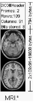
Most of the dMRI scanner produces data in DICOM format (.dcm - Dig-ital Imaging and Communications in Medicine). DICOM is the most common standard for receiving scans from a hospital [10, 67, 70]. The DICOM standard was created by the National Electrical Manufacturers Association (NEMA)1 to aid the distribution and viewing of medical im-ages, such as CT scans, MRIs, and ultrasound. A single DICOM file con-tains both a header (which stores information about the patient’s name, the type of scan, image dimensions, etc), as well as all of the image data (which can contain information in three dimensions) [45].
Figure 2.1 shows an example of the hypothetical DICOM image file. In this one, DICOM header uses the first 794 bytes to describe the im-age dimensions and retain other text information about the scan. The size of this header varies depending on how much header information is stored. For example, in the Figure 2.1, the header defines an image which has the dimensions 109×91×2voxels, with a data resolution of 1 byte per voxel, and the total image size will be 19838. Following the
header is the image data, and both the header and the image data are
Diffusion magnetic resonance imaging (dMRI) data and deterministic tractography 15
Figure 2.1: An example of the DICOM image file. The image is reproduced fromhttp: //www.cabiatl.com/mricro/dicom/
stored in the same file. More information about DICOM format can be found on the official webpage of DICOM2.
Although DICOM is the most common standard for receiving scans, it is quite complex format, and difficultly to be understood. DICOM data, thus, needs to be converted in the format of NIfTI (Neuroimag-ing Informatics Technology Initiative) [108]. NIfTI is a modern incar-nation of the Analyze format, but includes important information like the orientation of the image [22]. It was for scientific analysis of brain images 3. The images can be stored as a pair of files (hdr/img, compli-ant with most Analyze format viewers), or a single file (nii). Many tools like FSL [49], NiBabel4, MRIcron5, . . . are also able to read compressed (nii.gz) images. NIfTI format attempts to keep spatial orientation in-formation, therefore, it should reduce the chance of making left-right errors.
2http://medical.nema.org/
3http://nifti.nimh.nih.gov/
4http://nipy.org/nibabel
Figure 2.2: Image acquired orthogonal to scanner bore
When converting image from DICOM format to NIfTI format, beside the NIfTI file image, most of DICOM image conversion tools also gen-erate (.bvec) and b-value (.bval) text files (contains diffusion gradient vector and the b-value). These files are very important to reconstruct diffusion properties. Because in diffusion tensor imaging (DTI) method, we construct tensors by collecting a series of direction-sensitive diffu-sion images [6]. Therefore, in addition to recording the images, the scan-ner also saves these directions. A potential concern is that the scanscan-ner manufacturers can choose to either report the vectors with reference to the scanner bore, or with reference to the imaging plane (i.e., imaging grid). This is not a problem if the images are always acquired precisely orthogonal to the scanner bore (Figure 2.2), as the image and scanner have the same frame of reference. However, problems can arise when the image plane is not aligned with the scanner bore (i.e., oblique acqui-sitions). In this situation, it is important to ensure that these vectors are in the same frame of reference as the image. Moreover, the eigenvectors of the tensor, and consequently tractography programs are sensitive to proper interpretation of the bvecs relative to the imaging plane.
2.1.2 Reconstruction
Diffusion magnetic resonance imaging (dMRI) data and deterministic tractography 17
the spatial distribution of the diffusion signal within each voxel. While tracking tries to connect many signals to form a tractography based on orientation signal of each voxel.
It is usually to extract brain image only from the actual dMRI data in NIfTI images before doing reconstruction, because the result of scanner contains not only brain but also other things close to brain which can distract the processing of tracking. Brain extraction is the process of re-moving the skull and the rest of the head from the brain (see Figure 2.3). The resulting file only contains a representation of the brain’s anatomy.
Brain extraction can be done with the FSL 6 program BET (Brain Ex-traction Tool) [96]. BET takes an image of a head and removes all non-brain parts of the image. It uses a deformable model that evolves to fit the brain’s surface by the application of a set of locally adaptive model forces. This method is fast and requires no preregistration or other pre-processing before being applied. Result of BET is a file saved with a brain extension at its end. An example of BET result can be seen in the bottom line of the Figure 2.3, while original image data is at the top.
After brain extraction, we can do reconstruction step. The main pur-pose of this is to estimate the orientation information from the diffusion signal within each voxel which is adequate for accurate tractography generation. In the last few years, there has been an increasing number of techniques which are proposed to recover the signal directions inside the voxel from dMRI data, and the most simple one is Diffusion Tensor Model [6]. But in many cases this model is not sufficiently [2], because most of voxels inside brain contain multiple streamline bundles cross-ings while this model is only working with single tensor. Many other reconstruction methods have been proposed to overcome the limitations of this Diffusion Tensor model, such as Diffusion Spectrum Imaging [14]
Figure 2.3: An example of the dMRI data after doing brain extraction. Top: the original NIfTI images. Bottom: the result of doing brain extraction
or Higher Order Tensors [80]. The overview of these model can be found more detail in [42].
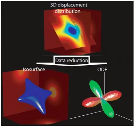
To visualize the 3D diffusion data, [42] proposed two approaches. The first one is to replace the displacement distribution with an isosur-face, which is a surface that passes through all points of equal probabil-ity densprobabil-ity value. And the second one is to compute the orientation dis-tribution function (ODF) from the displacement disdis-tribution. Figure 2.4 represents these two approaches.
2.1.3 Tracking
proce-Diffusion magnetic resonance imaging (dMRI) data and deterministic tractography 19
Figure 2.4: Two approaches maybe used to simplify the visual representation of 3D diffusion data. Top: the reconstruction of the3D displacement probability distribution from the diffusion signal. Left: the replacement of the displacement distribution with an isosurface. Right: the computation of the commonly used Orientation Distribution Function (ODF). This displacement distribution simulates the crossing of two fibres. In general, the ODF is used essentially to identify the primary directions of the underlying fibres. Picture is reproduced from [42]
dure consists of starting at a seed location and following the preferred direction until we reach a new voxel. Then, we can change to this vox-els referred direction and continue until an entire track is propagated. An example about creating track from orientation of streamline signal within voxels is presented in Figure 2.5
Figure 2.5: Tracking from tensor direction information. The white line shows the streamline obtained by joining a set of voxels based on their diffusion direction in-formation. The color is a complementary way of coding the preferred direction where red denotes left-right, green denotes back-front and blue denotes up-down. Picture is produced from [30]
the need of creating the whole brain tractography, only local techniques are described in this part.
Tractography segmentation 21
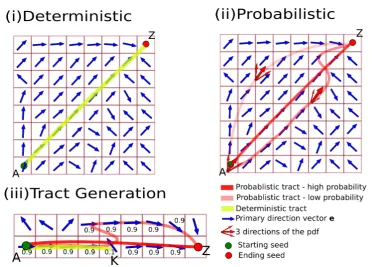
Figure 2.6: A simplified example showing in (i) and (ii) the same data set. (i) The yellow line shows the result of deterministic tractography which is given by a single trajectory and in (ii) is given by connectivity matrix depicting in red the probability of different pathways throughout the hole slice. For the ease of understanding, only 3 possible pathways are depicted. Finally, in (iii) an example is given where it is shown that probabilistic tractography weights more closer connections. However, it can track further deep than deterministic tractography. Picture is produced from [30]
2.2
Tractography segmentation
Alzheimer disease. Traditionally, the segmentation task is done by neu-roanatomists, and it consumes a lot of time and effort due to the large number of streamlines (about 3×10⁵ in a normal brain). Moreover, the variability of the brain anatomy among different subjects makes this task more difficult. Furthermore, clinical studies often use the segmentation of white matter bundles in order to perform comparisons between pop-ulations, and thus, it is also an press on the accuracy of the segmentation task. Therefore, . Recently, there is a rise of applying pattern recognition techniques to solve this problem [73, 111, 75], however the segmentation of tractography is still not completely solved problem. In the following part, the brief survey about currently trends in segmentation tractogra-phy is presented.
Atlas approach: Atlas are the models of white mater structure in
brain. Firstly, atlas are created from experience of experts without be-ing driven from data. After that, atlas are used as model of clusters for tractography segmentation. All streamlines would be grouped into the closest cluster in atlas. O’Donnell and Westin [73] generated a tracto-graphic atlas using spectral embedding and expert anatomical labeling. They then automatically segmented the new tractography using again spectral clustering and embedding the tracks as points in the embed-ded space, to the closest existing atlas clusters. The true affinity matrix was too big to compute therefore they used the Nystrom approximation: working on a subset and avoid generating the complete distance matrix. However, the important information from the full data set may be lost after sub-sampling.
ROI - region of interest: One of the first idea for segmentation is to
re-Tractography segmentation 23
quires to specified manually some regions where tracts start, end or pass through. Then streamlines would be filtered based on the constraint of passing through ROIs. ROI approach needs a prior knowledge about the trajectory and is used only for well-characterized white matter tracts. In order to refine the segmentation, multi-ROIs were used to include or exclude tracks.
Unsupervised learning: From the point of view of algorithmic
ap-proaches, the segmentation task has traditionally been addressed with unsupervised techniques over only diffusion data [111]. This typical framework first defines a pairwise distance between fibers and inputs the similarity matrix to standard clustering algorithms. Various distance functions between fibers have been proposed: the Euclidean distances between fiber shape descriptors [13]; the similarity between two fibers based on the number of points sharing the same voxel [50]; distance from the B − spline representation [63]; closest point distance, mean of closest distances and Hausdorff distance [33]. Then, following is a clustering algorithm such as agglomerative, k-means, Gaussian mixture model, etc (see [105] for a recent brief review of applying these algorithm for tractography).
lin-ear programming to chose the number of clusters. Recently, Garyfallidis et al. [32] proposed a very quick clustering algorithm, called QuickBun-dles. It took one random streamlines as initial cluster, and calculated the distance from all the un-clustered streamlines to the representatives of clusters. Only the streamline with the minimum distance was grouped into the closest cluster if the distance was less than a given threshold, other while, that streamline became a new cluster.
Although these approaches avoid manually choosing number of clus-ter, the drawback is the high space and time complexity of computing pairwise distances between fibers. Whole brain tractography produces
≈ 3× 10⁵ streamlines fibers per subject, the pairwise distance between fibers is difficult to compute. And it becomes more serious when clus-tering fibers of multiple subjects. To avoid computing pairwise dis-tances between fibers, Savadjiev et. al. [93] clustered diffusion orien-tation distribution functions maxima instead of clustering fiber tracts directly. This algorithm based on the geometric coherence of fiber ori-entations. Maddah et al. in [64] proposed a probabilistic approach to cluster fibers. It used a Dirichlet distribution as a prior to incorporate anatomical information. However, this algorithm also required estab-lishing point correspondence which was difficult to define.
Supervised learning: The most disadvantage of unsupervised
Tractography segmentation 25
samples are used to train a classify model, which is used to cluster a new streamline. In this setting, each streamline can be class-labelled as being member of the fiber tract of interest or not. For this reason the super-vised segmentation problem becomes a binary classification problem. Maddah et al. [63] used the B-spline representation of the streamlines, and classified by the nearest-neighbor algorithm with respect to an at-las. Wang et al. [105] proposed a non-parametric Bayesian framework using a hierarchical Dirichlet processes mixture (HDPM) model, and the models of bundles were learned from how voxels are connected by fibers in training data instead of comparing fiber distances. Olivetti [77] combined both structural and functional connectivity to study jointly in a pairwise approach with the goal of assessing the contributions of structural information and functional information when segmenting the tracts. Recently, [75] solved this classification problem basing on the dis-similarity representation. After projecting all streamlines into some pro-totypes, one streamline-streamline distance function is computed in this new representation space, and it is used for classifying.
Although supervised approaches focus on a specific tract as requirement of medical practitioners. However, because the number of data for train-ing and testtrain-ing is very small due to the vague time for collecttrain-ing enough the truth background data of manual segmentation tractography, the re-sults usually are bellow the expectation of medical practitioners, and they need to be refined to use in clinical applications.
such a vectorial representation. The dissimilarity representation, a spe-cific Euclidean embedding technique, is usually used in the context of classification and clustering problems. It is defined by selecting a set of objects (e.g. a set of streamlines) called prototypes, and then by mapping any new object (e.g. anynew streamline) to the vector of distances from the prototypes. It is a lossy transformation in the sense that some infor-mation is lost when projecting the data into the dissimilarity space. To the best of our knowledge this loss, i.e. the degree of approximation, has received little attention in the literature. In [86] the approximation was studied to decide among competing prototype selection policies only for classification tasks. In this work we are interested in assessing and controlling this loss without restriction to the classification scenario.
2.3
Tractography registration
Current neuroscientific analyses of white matter tractography data are limited to qualitative intra-subject comparisons. Thus, it is quite difficult to use the information for direct inter-subject comparisons [37, 7]. This leads to the need of initial alignment, or registration, of tractographies together via some methods before doing further study.
Equa-Tractography registration 27
tion 2.1, which has12 degrees of freedom (DOF) in3D.
x0 y0 z0 1 =
l11 l12 l13 tx
l21 l22 l23 ty
l31 l32 l33 tz
0 0 0 1
x y z 1 (2.1)
where lij are the nine parameters of a linear transformation, the ti are
the translation parameters in 3D; x, y, and z are the input coordinates andx0, y0, and z0 are the transformed coordinates. Any registration tech-nique can typically be described by three components: a transformation, a similarity measure and an optimization. The transformation is applied to an input image to increase its similarity with the reference image. The similarity measure measures the similarity between the reference image and the input image after transforming. And the optimization algorithm iteratively determines the optimal transformation parameters as a func-tion of the similarity measure. Image registrafunc-tion plays an important role in medical image analysis, group analysis and statistical parametric mapping. Because of its importance in both research and medical ap-plications, medical image registration has been intensively investigated for almost three decades and numerous algorithms have been proposed. More detail can be found in the recent survey of medical image registra-tion in [65].
registration, there are three alternative approaches: scalar or vectorial registration, tensor registration and fiber or streamline registration. We choose to keep the registration based on data type to elaborate.
From scalar image based registration point of view, mutual infor-mation is used to measure the similarity between images. Affine co-registration along with mutual information is performed with diffusion weighted images [62]. Orientation information of the diffusion tensor preserves after affine transformation in order to align anatomical struc-ture. Scalar registration are used at early stage of dMRI registration with the scaler images; without considering the directional images. More de-tails can be found in [82, 35].
In tensor based method [92], FA (Fractional Anisotrophy) mapping or affine registration is applied on tractography along with tensorial value of the images. We can distinguished tensor based registration with the scalar registration by additional deformation model which keep the tensor orientation consistent according to the anatomical structure of the image. Direct and feature based methods are discussed in [92], where direct approach is based on Diffusion Tensor Constancy Con-straint (DTCC) along with finite strain reorientation schema, and feature based method is based on singular value decompositions (SVD). Above described image based and tensor based model are voxel based registra-tion and by considering the anatomical images, not on 3D reconstructed tractography.
rea-Tractography registration 29
Figure 2.7: Tractography registration: voxel based method and tract-based method
In streamline registration, streamline is usually considered as a set of points [66, 59, 115]. Points are represented in high dimensional point space. In [66], Efficient Interactive Closest Feature point (ICF) is used to register different tractographies. Computational complexity on high dimensional search is handled by implementing approximate nearest neighbors techniques. In [115], streamlines are projected on high di-mensional feature space with a 3D coordinates sequence. Fiber model is extracted by adaptive mean shift (AMS) clustering. Gaussian Mixture Model (GMM) is represented by assigning weight to each fiber model. The registration is performed as the alignment of two GMMs by maxi-mizing the correlation ratio.
Recently another unbiased multi-subject registration is proposed in [72]. In that paper registrations are done by minimizing the entropy based objective function. Distance between the streamlines are calculated and represented by the Gaussian kernel distribution. This registration tech-nique works with the whole brain with group wise registration.
In this work, instead of finding the shape transformation of one trac-tography into another, we try to find which streamline in one tractogra-phy correspond to which streamline in the other tractogratractogra-phy, without any transformation. In other words, we try to find a mapping between the tractographies. The tractography mapping is similar to the well-known graph matching problem [18, 109] in pattern recognition litera-ture. During the last decade, graph matching has paid a huge attention due to the application of it in modern scientific discipline and applied field [61]. The graph matching problem can be described as follows. An undirected weighted graphG = (V, E) of sizeN is a finite set of vertices
V = {1, . . . , N} and edges E ⊂ V × V. Given two graphs GA to GB
with the same number of vertices N, the problem of matching GA and
Tractography registration 31
GB, which allows to align, or register, GA and GB in some optimal way.
The correspondence between vertices of GA and of GB is defined as a
permutation P of the N vertices, i.e. there a one-to-one correspondence between the two set of vertices. P is usually represented as a binary
N ×N matrix where Pij is equal to 1, if the ith vertex of GA is matched
to thejth vertex ofGB, otherwise 0.
In literature, efficient algorithms for finding the matching matrix P
can be either optimal or approximate methods [18, 36, 109, 110]. Opti-mal matching algorithms always find an exact solution if it exists, and have exponential time complexity in the worst case, which makes them unattractive for many applications. In contrast, approximate or subop-timal matching algorithms find the local minima of the matching cost with the polynomial time complexity respect to the number of nodes. Generally, there are no guarantees to reach the global minimum, but often the approximation is not very far from the global one [18]. Al-mohamad et. al. [3] solved the quadratic problem by using the simplex algorithm, while [90] used a method based on Lagrangian relaxation network. In [36], Gold et. al. proposed the graduated non-convexity assignment to avoid poor local optima. The relaxation of the discrete optimization problem to be continuous one for the graph-matching was introduced in [109, 110]. Recently, a new graph matching algorithm has proposed with the exploration of factorizing affinity matrix in [112].
By considering each streamline as a vertex and the edge connecting vertex si and sj as the distance between the two streamlines, d(si, sj)
dif-ferent volume, motivates this difference. Secondly, in general there is not a one-to-one correspondence between the streamlines but a many-to-one correspondence. This is anatomically likely if we consider that a given anatomical structure (tract), e.g. the cortico-spinal tract (CST), whose streamlines should have direct correspondence across subjects, may have different number of streamlines. In this case, for example, multiple streamlines of one CST would correspond to a single streamline in the other CST. Because of these differences, it is generally not possible to directly apply efficient graph matching algorithms to the problem of mapping tractographies.
2.4
Notation
Let the polyline s = {x~1, . . . , ~xns}, where ~x ∈ R
3, be a streamline (or fiber,
track) reconstructed from dMRI data by deterministic tractography al-gorithms [69]. Note that each streamline has a different number of 3D points with other streamlines. Let the tractography T = {s1, . . . , sn} be
defined as a set of n streamlines. Current dMRI techniques operated on adult humans generate tractography of size in the order of 3 × 10⁵ streamlines. Let τ be an anatomical fiber tract of interest, e.g. the cor-tical spinal tract (see figure 5.13), and let T ⊂ T be its corresponding streamline-based approximation within given the tractography.
In the literature of tract segmentation or registration, it usually refers to distances between pair of streamlines as a leading way to incorpo-rate domain specific information. The recent survey about streamline distance can be found more detial in [111]. A popular group of dis-tances is the modified Hausdorff disdis-tances [26] and among the most popular [111] are
• d1(sA, sB) = n1
sA
PnsA
Notation 33
s
AB
s
Figure 2.8: Many distances between two streamlines, sA and sB (solid line), that are proposed in the literature are based on the set of minimum distances between each point ofsAtosB. The set of minimal distances is represented here as dotted lines.
• d2(sA, sB) = mini=1,...,nsAd(xAi , sB)
• d3(sA, sB) = maxi=1,...,nsAd(xAi , sB)
where (see Figure 2.8)
d(xAi , sB) = min j=1,...,nsB||x
A i −x
B
j ||2 (2.2)
which can be combined in order to get the symmetric versions:
• ha(d, sA, sB) = d(sA,sB)+2d(sB,sA)
• hb(d, sA, sB) = min(d(sA, sB),d(sB, sA))
• hc(d, sA, sB) = max(d(sA, sB),d(sB, sA))
Note that all distances defined above are not metric [26] becaused(sA, sB) =
Chapter 3
Dissimilarity Representation for
Tractography
3.1
Introduction
Deterministic tractography algorithms [69] can reconstruct white mat-ter fiber tracts as a set of streamlines, also known as tracks, from diffu-sion Magnetic Resonance Imaging (dMRI) [6] data. A streamline is a mathematical approximation of thousands of neuronal axons expressing anatomical connectivity between different areas of the brain, see Fig-ure 3.1. Recently there has been an increase of attention in analysing tractography data by means of machine learning and pattern recogni-tion methods, e.g. [111, 105]. These methods often require the data to lie in a vectorial space, which is not the case for streamlines. Stream-lines are polyStream-lines in 3D space and have different lengths and numbers of points. The goal of this work is to investigate the features and limits of a specific Euclidean embedding, i.e. the dissimilarity representation, that was recently applied to the analysis of tractography data [75].
The dissimilarity representation is an Euclidean embedding technique defined by selecting a set of objects (e.g. a set of streamlines) called prototypes, and then by mapping any new object (e.g. any new stream-line) to the vector of distances from the prototypes. This representa-tion [88, 5, 16] is usually presented in the context of classificarepresenta-tion and clustering problems. It is alossytransformation in the sense that some in-formation is lost when projecting the data into the dissimilarity space. To the best of our knowledge this loss, i.e. the degree of approximation, has received little attention in the literature. In [86] the approximation was studied to decide among competing prototype selection policies only for classification tasks. In this work we are interested in assessing and controlling this loss without restriction to the classification scenario.
Methods 37
Figure 3.1: A set of100streamlines, i.e. an example of prototypes, from a full tractog-raphy
collections of objects that do not have a natural vectorial space represen-tation. The lack of the vectorial representation avoids the use of some of those algorithms and of computationally efficient implementations. The dissimilarity space representation could be the way to provide such a vectorial representation and for this reason it is crucial to assess the degree of approximation introduced. Besides this characterisation we propose the use of a stochastic approximation of an optimal algorithm for prototype selection that scales well on large datasets. This scalability issue is of primary importance for tractographies given that a full brain tractography is a large collection of streamlines, usually≈ 3×10⁵, a size for which algorithms may become impractical. We provide practical ex-amples both from simulated data and human brain tractographies.
3.2
Methods
3.2.1 The dissimilarity projection
Let X be the space of the objects of interest, e.g. streamlines, and letX ∈ X. Letd :X ×X 7→ R+be a distance function between objects inX. Note that d is not assumed to be necessarily metric. Let Π = {X˜1, . . . ,X˜p},
where ∀i X˜i ∈ X and pis finite. We call each X˜i as prototypeor landmark.
The dissimilarity representation/projection is defined as φdΠ(X) : X 7→ Rp
s.t.
φdΠ(X) = [d(X,X˜1), . . . , d(X,X˜p)] (3.1)
and maps an object X from its original spaceX to a vector of Rp.
Note that this representation is a lossy one in the sense that in gen-eral it is not possible to exactly reconstruct X fromφdΠ(X)because some information is lost during the projection.
We define the distance between projected objects as the Euclidean dis-tance between them: ∆dΠ(X, X0) =||φdΠ(X)−φdΠ(X0)||2, i.e. ∆dΠ : X ×X 7→
R+. It is intuitive that ∆dΠ and d should be strongly related. In the fol-lowing sections we will present more details and explanations about this relation.
3.2.2 A measure of approximation
We investigate the relationship between the distribution of distances among objects in X through d and the corresponding distances in the dissimilarity representation space through ∆dΠ. We claim that a good dissimilarity representation must be able to accurately preserve the par-tial order of the distances, i.e. if d(X, X0) ≤ d(X, X00) then ∆dΠ(X, X0) ≤
Methods 39
possible pairs of objects inX:
ρ = Cov(d(X, X
0),∆d
Π(X, X0))
σd(X,X0)σ∆d
Π(X,X0)
(3.2)
where X, X0 ∼ PX. In practical cases PX is unknown and only a finite
sample S is available. We can approximateρ as the samplecorrelation r
where X, X0 ∈ S. An accurate approximation of the relative distances between objects inX results in values of ρ far from zero and close to11.
In the literature of the Euclidean embeddings of metric spaces, the term of distortion is used for representing the relation between the dis-tances in the original space and the corresponding ones in the projected space. The embedding is said to havedistortion≤ c if for everyx, x0 ∈ X:
d(x, x0) ≥ ∆dΠ(x, x0) ≥ 1
cd(x, x 0).
(3.3)
An interesting embedding of metric spaces is described in [60]. It is based on ideas similar to the dissimilarity representation and has the advantage of providing a theoretical bound on the distortion. Unfortu-nately this embedding is computationally too expensive to be used in practice.
We claim that correlation and distortion target are slightly different aspects of the embedding quality, the first focuses on the averaged dif-ferences between the original and projected space, and the second on the worst case scenario. For this reason we claim that, in the context of machine learning and pattern recognition applications, correlation is a more appropriate measure.
3.2.3 Strategies for prototype selection
The definition of the set of prototypes with the goal of minimising the loss of the dissimilarity projection is an open issue in the dissimilarity space representation literature. In the context of classification problems the policy of random selection of the prototypes was proved to be use-ful under certain assumptions [5]. In the following we address the issue of choosing the prototypes in order to achieve the desired degree of ap-proximation but we do not restrict to the classification case only. We de-fine and discuss the following policies for prototype selection: random selection, farthest first traversal (FFT) and subset farthest first (SFF). All these policies are parametric with respect to p, i.e. the number of proto-types.
Random Selection
In practical cases we have a sample of objects S = {X1, . . . , XN} ⊂ X.
This selection policy draws uniformly at random from S, i.e. Π ⊆ S
and |Π| = p. Note that sampling is without replacementbecause identical prototypes provide redundant, i.e. useless, information. This policy was first proposed in [29] for seeding clustering algorithms. This policy has the lowest computational complexity O(1).
Farthest First Traversal (FFT)
Experiments 41
can find an -cover2 of S of size k? 3. The k-center problem is known to be an NP-hard [44], i.e. no efficient algorithm can be devised that always returns the optimal answer. Nevertheless FFT is known to be close to the optimal solution, in the following sense: IfT is the solution returned by FFT and T∗ is the optimal solution, then maxx∈Sd(x, T) ≤
2 maxx∈S d(x, T∗). Moreover, in metric spaces, any algorithm having a
better ratio must be NP-hard [44]. FFT has O(p|S|) complexity. Unfor-tunately when|S|becomes very large this prototype selection policy be-comes impractical.
Subset Farthest First (SFF)
In the context of radial basis function networks initialisation, a scalable approximation of the FFT algorithm, calledsubset farthest first(SFF), was proposed in [100]. This approximation is also claimed to reduce the chances to select outliers that can lead to a poor representation of large datasets. The SFF policy samplesm = dcplogpepoints fromSuniformly at random and then applies FFT on this sample in order to select the p
prototypes. In [100] it was proved that under the hypothesis of p clus-ters in S, the probability of not having a representative of some clusters in the sample is at mostpe−m/p. The computational complexity of SFF is
O(p2logp). Note that for large datasets and smallpthis prototype selec-tion policy has a much lower computaselec-tional cost than FFT.
3.3
Experiments
In the following we describe the assessment of the degree of approxi-mation of the dissimilarity representation across different prototype
se-2Given a metric space(X, d), for any >0, an-cover of a setS ⊂ X is defined to be any setT ⊂X such thatd(x, T)≤,∀x∈S. Hered(x, T)is the distance from pointxto the closest point in setT.
3 2 1 0 1 2 3 4 5 3
2 1 0 1 2 3
Figure 3.2: A 2-dimensional example of 50 points (black circles) drawn from N(0, I) and3prototypes (red stars) drawn from the same pdf.
lection policies and different numbers of prototypes. The aim is to in-vestigate the trade-off between accuracy and computational cost. The experiments are carried out on 2D simulated data and on real tractogra-phies reconstructed from dMRI recordings of the human brain.
3.3.1 Simulated data
LetX = R2,PX = N(µ,Σ),µ = [0,0],Σ = I,d(X, X0) = ||X−X0||2,p = 3
andX˜1,X˜2,X˜3 ∼ PX. ThenφdΠ(X) = h
||X −X˜1||2,||X −X˜2||2,||X −X˜3||2 i
∈
R3. Figure 3.2 shows a sample of50points drawn fromPX together with
the 3 prototypes X˜1,X˜2,X˜3. Figure 3.3 shows the sample projected into the dissimilarity space together with the prototypes.
Experiments 43
1 2
3 4 5
0.5 1.0 1.5 2.0 2.5 3.0 3.5 4.0 0.5 1.0 1.5 2.0 2.5 3.0 3.5 4.0
Figure 3.3: The dissimilarity projection of the dataset and prototypes of Figure 3.2.
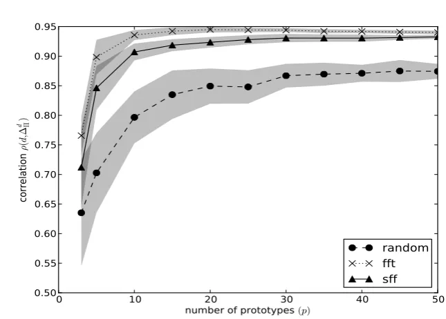
between distances in the original space and the corresponding distances in the projected space was estimated by computing50repetitions of the simulated dataset. The average correlation and one standard deviation for each prototype selection strategy are shown in Figure 3.5.
In this simulated dataset both SFF and FFT performed significantly better than the random selection, on average. FFT showed a small ad-vantage over SFF whenp < 10.
3.3.2 Tractography data
0 1 2 3 4 5 6 7
d(x,x0)
0 1 2 3 4 5 6 ∆
d (Π
x,
x
0
)
Figure 3.4: The correlation distances of 50points (2D dimention) in original space (d
x-axis) and in the projection space (∆d
Πy-asix) with random prototype selection policcy.
0 5 10 15 20
number of prototypes (p)
0.3 0.4 0.5 0.6 0.7 0.8 0.9 1.0 co rre lat ion ρ ( d, ∆
d)Π
random fft sff
Experiments 45
EuDX, a deterministic tracking algorithm [30] from the DiPy library 4. We obtained two tractographies using 104 and 3× 10⁶ random seed re-spectively. The first tractography consisted of approximately103 stream-lines and the second one of3×105 streamlines. An example of a set of prototypes from the largest tractography is shown in Figure 3.1.
As the distance between streamlines we chose one of the most com-mon, i.e. the symmetric minimum average distance from [111] defined asd(Xa, Xb) = 12(δ(Xa, Xb) + δ(Xb, Xa)) where
δ(Xa, Xb) =
1
|Xa|
X
xi∈Xa min
y∈Xb
||xi−y||2. (3.4)
As it is shown in Figure 3.6 for the case of a tractography of 103 streamlines both FFT and SFF(c = 3) had significantly higher correlation than the random sampling for all numbers of prototypes considered. We confirmed that the SFF selection policy is an accurate approxima-tion of the FFT policy for tractographies. Moreover we noted that after 15− 20 prototypes the correlation reaches approximately 0.95 on aver-age (50 repetitions) and then slightly decreases indicating that a little number of prototypes is sufficient to reach a very accurate dissimilarity representation.
Figure 3.7 shows the correlation for SFF and the random policy when the tractography has3×105 streamlines, i.e. the standard size of a trac-tography from current dMRI recording techniques. In this case FFT is impractical to be computed because it requires approximately 15 min-utes on a standard desktop computer for a single repetition whenp = 50. The cost of computing SFF is instead the same of the case of103 stream-lines, as its computational cost depends only on the number of proto-types. It took ≈ 2 seconds on standard desktop computer when p = 50
0 10 20 30 40 50
number of prototypes (p)
0.50 0.55 0.60 0.65 0.70 0.75 0.80 0.85 0.90 0.95 co rre lat ion ρ ( d, ∆
d)Π
random fft sff
Figure 3.6: The correlation between of d and ∆d
Π over a 103 streamlines tractography for different prototype selection policies.
to compute one repetition. We observed that for 3×10⁵ streamlines SFF significantly outperformed the random policy and reached the highest correlation of 0.96 on average (50repetitions) for15−25prototypes.
Note that the figures presented in this section refers to data from sub-ject1of the dMRI dataset. We conducted the same experiments on other subjects obtaining equivalent results.
3.3.3 Dissimilarity for fast clustering tractography
Experiments 47
0 10 20 30 40 50
number of prototypes (p)
0.50 0.55 0.60 0.65 0.70 0.75 0.80 0.85 0.90 0.95 co rre lat ion ρ ( d, ∆
d)Π
random sff
Figure 3.7: The correlation between of d and ∆d
Π for a full tractography of 3× 10⁵ streamlines with random, and SFFprototype selection policies.
in the endeavour of characterisation of the ALS disease is to segment the CST from the full brain tractography of each subject.
Tractography segmentation can be performed manually or automat-ically. Despite an increasing literature in automatic segmentation (see a brief review in [105]), the application in the clinical domain usually still rely on manual segmentation. The manual segmentation process usu-ally consists in selecting the subset of the streamlines connecting a few manually located regions of interest5. This task is a lengthy and complex one due to a very large set of streamlines in tractography, in the order of 3× 10⁵, which makes it intrinsically difficult both to inspect and to unfold anatomical structures.
In this part, we conceived a novel computer-assisted interactive pro-cess based on clustering algorithms with the help of dissimilarity rep-resentation, and aimed at greatly reducing the time required to
ally segment a given anatomical white matter structure of interest. Our approach is based on a fast-clustering technique based on dissimilarity representation, by means of which the expert is presented with a sum-mary of the streamlines, i.e. the clusters represented by their medoids 6. The expert manually selects the medoids/clusters of interest in order to remove most of the streamlines not related to the anatomical structure of interest. Interacting with the summary, instead of the actual stream-lines, is much simpler for the user. In this part, we only mention the fast clustering based on dissimilarity, the more detail of the interactive segmentation procedure can be found in the Chapter 5.
The core of the problem is to cluster a large number of streamlines in no more than a few seconds, to allow a comfortable interactive user experience to the expert. The proposed solution combines two state-of-the-art elements: first a recently proposed Euclidean embedding algo-rithm for streamlines, i.e. the dissimilarity representation with the scal-ablesubset farthest first(SFF) prototype selection policy [76]. This embed-ding provides fast and accurate vectorial representation of streamlines. Second, a recently proposed improvement of the k-means clustering al-gorithm called mini-batch k-means [94] (MBKM). This algorithm, which require the data to lie in a vector space, drastically reduces the conver-gence time to the actual clusters in case of large and very-large sets of objects. We claim that the dissimilarity embedding together with the MBKM algorithm provides a viable solution to problem of fast cluster-ing of streamlines.
Mini-Batchk-means
The k-means clustering problem is a cornerstone of the clustering liter-ature. Given k, the number of clusters, the problem is to find k
Experiments 49
ter centres C = {c1, . . . ,ck}, c ∈ Rp, and to assign each element of
the vectorial dataset Φ(T) = {φ(X1), . . . , φ(XM)} ⊂ Rp to the closest
cluster7. The k-means problem is then to compute centres C such as to minimise the loss function f(C) = P
φ(X)∈Φ(T)D(φ(X), C)
2, where
D(φ(X), C) = minc∈C||φ(X) − c||2 is the distance between φ(X) and the closest centre. The exact solution of the k-means problem is N P -hard and the computational complexity of the standard algorithm, the Lloyd’s algorithm, has been proved to beO(M34) in the general case [4], even though much less in practical applications.
Themini-batchk-means(MBKM) algorithm [94] is a recently proposed modification of the standard algorithm that is able to reduce the com-putational costs by orders of magnitude. The intuitive idea is to use a stochastic gradient descent approach to find the centresC starting from a random initialisation. This idea was introduced in [11] where the points of the dataset were given one at a time in an online fashion.
Instead of updating the centers with one streamline at a time, the MBKM algorithm proposes