Efficient Temporal Pattern Mining for Humanoid Robot
Upasna Singh
Robotics and AI Lab
Indian Institute of Information
Technology, Allahabad.
91-532-292-2116/2120
[email protected]
G C Nandi
Robotics and AI Lab
Indian Institute of Information
Technology, Allahabad.
91-532-292-2101/2094
[email protected]
ABSTRACT
Pattern mining in temporal databases is one of the challenging platform which holds attention when some ordered sequences are frequently occurred at different time instances in the dataset. We have found temporal patterns in humanoid robot dataset of HOAP-2 (Humanoid Open-Architecture Platform) which generates different motions through recurring sequences of various joint associations. For mining temporal patterns in that dataset we have proposed a method. This method uses FP-Temporal and SH(Soft-Hyperlinked)-FP-Temporal mining algorithm as pattern growth methods for generating temporal association rules for various motion patterns of HOAP-2. Brief performance analysis shows that SH-Temporal is much efficient than FP-Temporal for such datasets and works significantly for mining sequentially associative temporal patterns in terms of temporal association rules.
Keywords
Temporal Pattern Mining, HOAP-2 dataset, Temporal datasets, SH Temporal algorithm, Temporal association rules.
1.
INTRODUCTION
Temporal databases are the repositories having records with respect to time. The time information can be granulized either in terms of calendar units (day, month, year), clock units (min, hr, sec,) or scientific time units (milliseconds, nanoseconds etc.). The challenging task in such databases is to dredge frequently occurring temporal patterns that could discover knowledge for futuristic ontology based on those recurring occurrences. There are numerous techniques in data-mining for mining hidden patterns from bulky databases [10]. One such technique is Association rule mining [7, 3]. Earlier this technique was using Apriori algorithm for mining frequent patterns but later on it has been modified in terms of improved algorithms known as pattern growth methods and then mine association rules from the resulting frequent patterns. FP (Frequent Pattern) growth and H-mine are well known pattern growth methods for mining frequent patterns in transactional databases. Recently, we have found that SH-Struct (Soft-Hyperlinked Structure) is also a compatible structure for generating frequent patterns using SH-Mine algorithm [22]. For dealing with temporal databases, many extensions in various existing algorithms [2, 3, 4 , 5, 8, 12, 9] have been proposed so far. In this study, we have extended SH-Mine algorithm as SH-Temporal algorithm for temporal databases. It generates temporal patterns and then results in terms of temporal association rule which is purely depending on the
dataset. For implementation we have used HOAP-2 datasets. The existing algorithms for mining frequent patterns can be altered with respect to the dataset but the conceptual idea remains same.
In furtherance, we explained prerequisites in section II. Proposed method is briefly demonstrated in section III, and the experimentation is done over HOAP-2 dataset using SH-Temporal, the proposed algorithm is explained in section IV. Brief performance analysis and results have been discussed in section V. At the end overall study is concluded with its future application in section VI which is then followed by references.
2.
PREREQUISITES
2.1 Association Rule Mining
Agrawal, et. al. have proposed various algorithms favoring association rule mining since early 90’s [7]. According to them, it is a two-step process: first step is frequent pattern mining and then the next step is generating association rule from those frequent patterns. One of the fastest algorithm based on same property but using different time-saving tree-data-structure is FP(Frequent-Pattern) growth algorithm [1]. It generates frequent pattern without candidate generation using FP-tree recursively. After then H-Mine algorithm [11] have also attracted attention of many researchers since it is efficient for large datasets and space efficient. mine algorithm uses a new data structure called H-struct (Hyperlinked-H-structure) which dynamically adjusts the links for mining frequently occurred patterns.
For mining association rule from any transactional dataset like market-basket dataset, two constructs should be considered for accepting that rule: support and confidence. Let us assume if
A→B is an association rule, where A and B are disjoint subsets of
the items in the transactional dataset, then P(AUB) represents support of the rule and P(B|A) represents confidence of the rule. Among all the rules, the rule having support and confidence greater than or equal to minimum support and minimum confidence threshold respectively is considered to be the most prominent rule. Before mining association rule, frequent patterns are to be mined using any frequent pattern mining algorithm such as Apriori, FP- Growth, H-Mine, etc. Frequent pattern is also mined on the basis of support of the itemset (basically frequency of the itemset in the dataset). The itemset is said to be frequent if its support is greater than or equal to the minimum support threshold.
FP-Growth Algorithm uses Apriori Property and recursively
partitions the database into sub-databases according to the frequent pattern found .It searches local frequent patterns to
generate FP tree, the L-Order List and the Frequency List. For each transaction, the items are sorted in the decreasing order of their frequency of occurrence. The overall concept can be explained through an example as in figure 2. There are 5 transactions in which 5 items have been processed. According to the algorithm, the three-step process is followed which includes creation of Freq_List that stores frequency of each item throughout the dataset, creation of L_order List that maintains the criteria of minimum support threshold and then lastly obtain the FP_Tree of frequent items.
H-Mine Algorithm also uses Apriori Property. Like FP-growth, it
partitions search space according to both patterns and data set to be searched. Unlike FP-growth, it does not create physical projected items nor construct conditional FP-Trees, but it maintains H-Struct (Hyper-Linked Structure) for generating frequent patterns. Since H-Struct is space preserving, so it is memory efficient than FP-growth algorithm. In Figure 3, the same example of FP-growth is explained, so as to show that this algorithm preserves the ordering of the items and exempts the overhead of creating L_order List. It only maintains H-struct for every frequent itemset.
2.2 Temporal Pattern Mining
Temporal data mining is an important extension of existing data mining approach as it has the capability of mining activity rather than just states and, thus, inferring relationships of contextual and temporal proximity, for example to enquire the knowledge of cause-effect association. Generally, the accommodation of time into mining techniques provides a window into the temporal arrangement of events and, thus, an ability to suggest cause and effect that are overlooked when the temporal component is ignored or treated as a simple numerical attribute. Moreover, temporal data mining has the ability to mine the behavioral aspects of objects as opposed to simply mining rules that describe their states at a point in time. Also, through continuous research in this area, it was noticed that one important problem that arises during the discovery process is treating data with temporal dependencies. The attributes related with the temporal information present in this type of datasets need to be treated differently from other kinds of attributes. However, most of the data mining techniques tend to treat temporal data as an unordered collection of events, ignoring its temporal information.
2.2.1 Types of Temporal Databases
Temporal database is not essential for temporal knowledge discovery and that temporal rules can also be derived from sequences of static data sets. Thus, Roddick in [16] have defined four major types of temporal databases:
• Static: No temporal context is included.
• Sequences: Ordered list of events, but no timestamps
collections of events.
• Time-Stamped: A timed sequence of static data at regular
intervals.
• Fully-Temporal: Each tuple in a time-varying relation may
have one or more dimensions of time.
According to [13], Temporal Database is a relational database that includes time-related attributes that may include several timestamps having different semantics. Also, unlike traditional
KDD ontology, Roddick have defined new temporal Knowledge Discovery phases for discovering similarities in temporal data as:
• Data-Type (Static, Sequence, Time-Stamped, Fully
Temporal)
• Mining Paradigms (Apriori-discovery, Classification)
• Ordering (Temporal Association Rules)
It explains that when any of the kind of temporal dataset has taken for mining patterns, the extended Aprriori-like rule discovery process, Classification or Clustering tasks can be done according to data type to generate sequential or ordered, causal, cyclic, co-relational temporal association rules.
2.2.2 Temporal Association Rule Mining
In the transactional datasets when the transaction time is included then it is means that some information could be there which depends on time. Thus to retain the dynamic behaviour of that dataset, it would rather mandatory to search that information which is time-dependent or independent. But it is not easy when the dataset is in terabytes. Major concept of generating temporal association rule comes from temporal data-mining. This process is also similar to association rule mining having two tasks, mining of temporal frequent patterns and then generating temporal association rules. Temporal patterns could be mined through several approaches like Sequential Patterns[6], Periodic Patterns [20] , Calender-based Patterns [14, 15], Cyclic Patterns [21]. A
cyclic rule is one that occurs at regular time intervals, it means the transactions that support specific rules occur periodically. In order to discover these rules, it is mandatory to search for them in a particular portion of time, since they may occur repeatedly at specific time instants but on a little portion of the global time considered. As discussed above, the method to discover such
rules is applying an algorithm similar to the apriori, and after
having the set of traditional rules for detecting the cycles behind the rules. More efficient approach to discover cyclic rules consists on reversing the process: first discover the cyclic
large itemsets and then generate the rules. This kind of natural
extension to this method consists in allowing the existence of different time granularities, such as days, weeks or months, and is achieved by defining calendar algebra to define and manipulate groups of time intervals. The rules discovered are designated
calendric association rules. A different approach to the discovery of relations in multivariate time sequences is based on the definition of N-dimensional transaction databases. Transactions in such databases are obtained by discretizing, if necessary, continuous attributes. Hence, this type of databases can then be
mined to obtain association rules. However, new definitions for
association rules, support and confidence are necessary for
different kinds of datasets.
3.
PROPOSED METHOD
temporal confidence for mining frequent temporal patterns. In this paper, we have extended H-mine in terms of SH-Temporal Mine
(Soft-Hyperlinked Structure) algorithm, that can useH-Struct
for
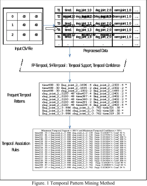
[image:3.612.51.298.182.495.2]building SH-Tree. That tree is implemented by using pointer-based linked list data structure. Overall implementation is explained in the followed subsection. FP-Temporal and SH-Temporal have produced same results in terms of frequent temporal patterns and then temporal association rules. But the performance analysis shows that SH-Temporal is much efficient than FP-Temporal in terms of space and time constructs.
Figure. 1 Temporal Pattern Mining Method
4.
EXPERIMENTATION
4.1 Data Description
We have tested aforesaid methodology over the temporal dataset of HOAP-2. In this dataset we have several files for several motions of HOAP-2. Detailed description about HOAP-2 can be obtained from [18].The dataset file contains 27 attributes. Out of which, 25 attributes store the value of 25 joints of HOAP-2 as it has 25 degrees of freedom. Each value has certain maximum and minimum range. In the dataset, one transaction (or record) represents the movement of 25 joints in 1 millisecond. We are considering the dataset of various patterns for experimentation:
• Walk Pattern
• Sumo Pattern
• Bye-Bye Pattern
• May-I Pattern
• Traffic Signal Pattern
Overall taxonomy in terms of number of records, number of attributes, number of samples and size of each sample for every pattern are shown in Table 1.
Main objective of experimentation is to discover knowledge of intermediate patterns which are hidden inside different existing patterns of motion of humanoid robot joints.
Right now, we have analysed our method over Walk pattern and Sumo pattern which contains 26000 and 27000 records respectively .Since these two patterns are the standard patterns and also the longest among all patterns, thus we have chosen them for analysis. For both the patterns we are considering all 25 joints motion. Also, our analysis is based on the simulation framework Webots[19]. This platform provides various user-friendly frameworks of robotics. In this framework we load CSV(Comma Separated Value) file which contains the joint-values. Here, the row represents 1 milisecond and coloum represent joint value in decimal form (Joint angle could be either in degrees or in decimal form). According to simulation, we came to know that robot can follow any pattern according to control steps. For walk pattern the control step is of 25 millisecond and for sumo pattern it is of 16 miliseconds. For our analysis, we have divided overall dataset into timestamps as time1, time2, time3….so on. In case of walk pattern 1 timestamp is of 50 miliseconds i.e. 2 control steps of simulated robot, similarly in sumo pattern 1 timestamp is of 64 milisecons i.e. 4 control steps of simulated robot. In walk pattern, we enquired that robot is performing walk on the basis of some cyclic associations of some specific joint values at a particular instant of time. Also, there may be the possibilities that the robot can walk in different ways such as slow, fast, run etc. Thus in order to generate intermediate hidden patterns in terms of temporal association rules, we have to find out frequently
recurring sequences w.r.t. time in that pattern. Such type of
analysis in various existing patterns could help us to generate some new patterns also.
Table 1. Taxonomy of different motion patterns of HOAP-2
4.2 Input Dataset
Initially the HOAP-2 motion pattern was in terms of CSV format. But since for pattern-growth methods, text formats are most feasible, so we have converted that data into .txt formats.
4.3 Preprocessing
The input file contains 27 attribute but for generating any motion pattern 25 joints are associated in some way or the other. Thus we have removed 2 unused attribute from the original CSV file and take remaining 25 attributes. The remaining attribute set is given as
Walk
Pattern Pattern Sumo Bye-Bye Pattern Pattern May-I
Traffic Signal Pattern Number of Records 26000 27000 15300 2000 4000
Number of Attributes 27 27 27 27 27
Number of Samples 1 1 12 10 10
Size of each Sample 3.02 MB 1.97 MB 700 KB 145KB 250 KB
-90 -90 2
-60 -60 1
-30 -30 0
rleg_joint_3_-90 rleg_joint_2_-90 rleg_joint_1_2
rleg_joint_3_-60 rleg_joint_2_-60 rleg_joint_1_1
rleg_joint_3_-30 rleg_joint_2_-30 rleg_joint_1_0
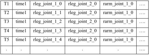
T1 time1 rleg_joint_1_0 rleg_joint_2_0 rarm_joint_1_0 …. T2 time1 rleg_joint_1_1 rleg_joint_2_0 rarm_joint_1_0 ….
T3 time1 rleg_joint_1_2 rleg_joint_2_0 rarm_joint_1_0 …. T4 time1 rleg_joint_1_3 rleg_joint_2_0 rarm_joint_1_0 ….
T5 time1 rleg_joint_1_4 rleg_joint_2_0 rarm_joint_1_0 ….
. . . . . ….
FP‐Temporal, SH‐Temporal : Temporal Support, Temporal Confidence
Frequent Temporal
Patterns
Temporal Association
Rules
[image:3.612.318.560.473.583.2]{rleg _joint_1, rleg _joint_2, rleg _joint_3, rleg _joint_4, rleg _joint_5, rleg _joint_6, rarm_joint_1, rarm_joint_2, rarm_joint_3, rarm_joint_4, lleg _joint_1, lleg _joint_2, lleg _joint_3, lleg _joint_4, lleg_joint_5, lleg _joint_6, larm_joint_1, larm_joint_2, larm_joint_3, larm_joint_4, body_joint_1}
[image:4.612.53.300.229.321.2]Also the CSV data is in the form of numeric values. Seeing the raw data one couldn’t find any meaning in its associations and thus we have converted it into meaningful form by appending attribute name with its value. The resulting input file of motion patterns is given in Table 2. In this file we have 21 attributes, but for applying any of the pattern growth method, we have to append transaction ID and time attribute in the transactional dataset.
Table 2. Preprocessed Tranasactional Dataset
4.4 Pattern Growth Method
In section 3, we have discussed that existing pattern growth methods for transactional databases can be extended for temporal databases for finding temporal patterns. In [17], we have defined temporal support and temporal confidence and use FP-temporal algorithm for mining temporal patterns. Here, we have used same definitions nut use SH-Temporal for mining temporal patterns.
4.4.1 Proposed Algorithm: SH-Temporal
SH-Temporal works in three phases
• Build SH-Tree,
• Mine Temporal Frequent pattern on the basis of minimum
support threshold,
• Generate Temporal Association rule on the basis of
Temporal support and Temporal Confidence.
For simplification we have explained overall algorithm in terms of pseudo code which has demonstrated separately for each phase of the algorithm.
First phase of the algorithm is to build SH-Tree. It can be created by taking the dataset in the format shown in table I. For building SH-tree, the frequently occurred joint-values (items) are arranged
in descending order in a list called freqlist. That list is arranged
according to the minimum support threshold (min_supp), i.e., the support count (frequency) of every value should be greater than or equal to min_supp. After that H-struct (Hyper-linked Struct) is created for all the values by inserting headers of each transaction. Input:Sample Dataset
Output:SH-Tree
Build_SH_tree
{
Create_freqlist();
Create_freq_file(min);
Insert_headernodes();
Insert_nodes();
}
Now, the output of first phase is processed as an input to the second phase. In this phase, the major task is to mine frequent temporal pattern from SH-Tree. From above we see that SH-Tree differs from FP-tree as it does not contain L-order list but it maintains H-struct at each level of the tree since it have to retain the order of the sequence of joints. H-struct contains three fields: item, its support count and its link to another frequently occurred item associated with it. For mining frequent temporal patterns we start from the root node of SH-tree and apply depth-first approach. Input:SH-Tree
Output:Frequent Temporal Pattern
SH_Temporal_Mine(t)
{
Consider L(i) to be the level of SH- tree t .
Start from the header node at level 1.
frequent_ list= item at level 1;
for(i=1;i<=total no. of level; i++)
{
if (support(item at level L(i+1)) >=min_supp)
frequent_list(i+1)=frequent_list(i),item at L(i+1) ;
display frequent_list;
Repeat the process for all header nodes at level 1.
}
}
All the patterns are generated on the basis of minimum support threshold (min_supp). We have processed our dataset with min_supp=5. In the next and the last phase of the algorithm, these temporal patterns are taken as an input for generating temporal Association Rules. It can be implemented as:
Input: Temporal Frequent Patterns
Output: Temporal association Rule
SH_Temporal_Association_Rule_Mine( Dataset D )
{
Foreach pattern
{
Make time antecedent of the rule and the rest pattern as the consequent.
Calculate Temporal Support of rule ( time → A , B ) = n( time U A U B ) / no. of records.
Calculate Temporal Confidence of rule ( time → A , B ) = supp (time U A U B ) / supp ( time ).
}
Rules having greater support and confidence than the minimum specified will be accepted.
}
T1 time1 rleg_joint_1_0 rleg_joint_2_0 rarm_joint_1_0 …. T2 time1 rleg_joint_1_1 rleg_joint_2_0 rarm_joint_1_0 …. T3 time1 rleg_joint_1_2 rleg_joint_2_0 rarm_joint_1_0 …. T4 time1 rleg_joint_1_3 rleg_joint_2_0 rarm_joint_1_0 …. T5 time1 rleg_joint_1_4 rleg_joint_2_0 rarm_joint_1_0 ….
In the pseudo code we have seen that the temporal rule is mined on the basis of minimum temporal support (min_temporal_supp) and minimum temporal confidence (min_temporal_conf). It is also user dependent.
5.
RESULTS AND DISCUSSION
5.1
Generating Temporal Association Rules
After applying abovementioned algorithm and the definitions explained in [17] for generating temporal patterns in Walk Pattern, the result is in the form of temporal association rule as:
5.1.1 Rules generated after applying FP-Temporal
Algorithm in Walk Pattern
Rule 1: time432 : 49 -> larm_joint_3_2087 : 26052
larm_joint_4_-5228 : 26052 larm_joint_2_2087 : 26052 rarm_joint_2_-2091 : 26052 rarm_joint_3_-2090 : 26052 rarm_joint_4_5222 : 26052 rleg_joint_1_-3 : 25407 body_joint_1_1 : 1594 lleg_joint_1_-1 : 1583
Supp: 0.188085 % Conf: 98 %
Rule 2: time431 : 31 -> larm_joint_3_2087 : 26052 larm_joint_4_-5228 : 26052 larm_joint_2_2087 : 26052 rarm_joint_2_-2091 : 26052 rarm_joint_3_-2090 : 26052 rarm_joint_4_5222 : 26052 rleg_joint_1_-3 : 25407 body_joint_1_1 : 1594 lleg_joint_1_-1 : 1583
Supp: 0.118993 % Conf: 62 %
5.1.2 Rules generated after applying SH-Temporal
Algorithm in Walk Pattern
Rule 1: time431 : 50 -> rleg_joint_1_-3 : 50 rarm_joint_2_-2091
: 50 rarm_joint_4_5222 : 50
Supp: 0.191924 % Conf: 100 %
Rule 2: time432 : 50 -> rleg_joint_1_-3 : 50 rarm_joint_2_-2091
: 50 rarm_joint_4_5222 : 50 larm_joint_3_2087 : 50 larm_joint_4_-5228 : 50 body_joint_1_1 : 50
Supp: 0.191924 % Conf: 100 %
Here the rule is of the form consequent -> antecedent, where consequent is the timestamp with frequency and the antecedent contains the recurring sequences of joint angle values with frequency. We have applied FP-Temporal and SH-Temporal to generate resulting rules shown above for Walk Pattern with minimum support threshold = .001 and minimum confidence threshold = 50 %. After doing the comparison study between these algorithm we have found that since in these rules ordering of the sequence is played an important rule, SH-Temporal would be more efficient than FP-Temporal when minimum support value is
less. Also, the rule length is small in case of SH-temporalwhereas
number of rules are less when we applied FP-Temporal.
5.2 Performance Analysis
This section explained how SH-Temporal is compatible with FP-Temporal for mining temporal patterns. All experiments have performed on WINDOWS 2000 with 3 GB ram and 32-bits operating system. We have implemented FP-Temporal for doing comparative analysis between the two algorithms. FP-Temporal generates same rules but use FP-Tree. The analysis is being done for different temporal supports w.r.t. time and space. From Figure
[image:5.612.320.557.114.222.2]2 and 3, we could easily make out that SH-Temporal performs faster than FP-temporal for generating temporal patterns of various joint trajectories.
[image:5.612.319.557.255.383.2]Figure 2. Time Analysis for mining Thigh Joint patterns using SH-Temporal and FP-SH-Temporal
[image:5.612.319.554.416.542.2]Figure 3. Time Analysis for mining Knee Joint patterns using SH-Temporal and FP-SH-Temporal
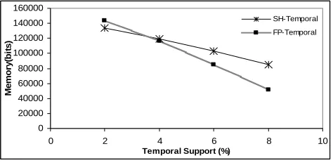
Figure 4. Memory requirements for storing Thigh Joint patterns using SH-Temporal and FP-SH-Temporal
Figure 5. Memory requirements for storing Thigh Joint patterns using SH-Temporal and FP-SH-Temporal
0 1 2 3 4 5 6 7 8 9 10
0 1 2 3 4 5 6 7 8 9
Tem poral Support (%)
R
un Ti
m
e
(
s
e
c
)
SH-Temporal FP-Temporal
0 2 4 6 8 10 12
0 2 4 6 8 10
Tem poral Support (%)
Ru
n Ti
m
e
(
s
e
c
)
SH-Temporal
FP-Temporal
0 20000 40000 60000 80000 100000 120000 140000 160000
0 1 2 3 4 5 6 7 8 9
Tem poral Support (%)
Me
m
o
ry
(b
it
s
)
SH-Temporal FP-Temporal
0 20000 40000 60000 80000 100000 120000 140000 160000
0 2 4 6 8 10
Temporal Support (%)
Mem
o
ry
(b
it
s)
[image:5.612.320.557.572.688.2]From Figure 4 and 5, we could say that for storing temporal
patterns of joints, SH-Temporal is good for less temporalsupport
i.e. when there are large no. of patterns, but as the temporal support increases less patterns are generated and in that case FP-Temporal is quite better. But still we could say that SH-FP-Temporal is a parallel approach like FP-Temporal to mine patterns from
temporal databases. These results we have analysed for Walk
Pattern. In the similar manner we can do the analysis for different
HOAP-2 patterns.
6.
CONCLUSION
The proposed method investigated that temporal pattern mining for HOAP-2 datasets is done through extended pattern growth methods. Overall results and performance study shows that the proposed SH-Temporal outperforms FP-Temporal when temporal support is less. In future, these algorithms can further be used and improved for gesture based classification for various HOAP-2 motions.
7.
REFERENCES
[1] Jiawei Han, Jian Pei, Yiwen Yin, "Mining Frequent Patterns
without Candidate Generation", Intl. Conference on
Management of Data, ACM SIGMOD,2000
[2] William Cheung, Osmar R. Zaiane, "Incremental Mining of
Frequent Patterns without Candidate Generation or Support
Constraint", Seventh International Database Engineering
and Applications Symposium (IDEAS'03), page-111, 2003
[3] Y. G. Sucahyo, R. Gopalan, “CT-PRO: A Bottom-Up Non
Recursive Frequent Itemset Mining Algorithm Using
Compressed FP-Tree Data Structure”, Proceedings of the
IEEE ICDM Workshop on Frequent Itemset Mining Implementations (FIMI), Brighton, UK, 2004.
[4] Christian Borgelt, “Keeping things simple: finding frequent
item sets by recursive elimination”, In Proc. of the 1st
international workshop on open source data mining: frequent pattern mining implementations, Chicago, Illinois, pages: 66 – 70, 2005.
[5] Mingjun Song, Sanguthevar Rajasekaran, "A Transaction
Mapping Algorithm for Frequent Itemsets Mining," IEEE
Transactions on Knowledge and Data Engineering, vol. 18, no. 4, pp. 472-481, Apr., 2006.
[6] Agrawal, Srikant: Mining sequential patterns. In: Proc.11th
Int. Conf. Data Engineering,Taipei, Taiwan, R.O.C., September 1995, pp. 3–14,1995.
[7] R. Agrawal, T. Imielienski, and A. Swami. “Mining
Association Rules between Sets of Items in Large Databases”, Proc. Conf. on Management of Data,207–216. ACM Press, New York, NY, USA 1993
[8] S. Ramaswamy, S. Mahajan, and A. Silberschatz. On the
discovery of interesting patterns in association rules. In Proc.
of the 1998 Int’l Conf. on Very Large Data Bases, pp 368– 379, 1998.
[9] R. Bayardo Jr., R. Agrawal, and D. Gunopulos."
Constraint-based rule mining in large, dense databases", In Proc. of
the15th Int’l Con$ on Data Engineering, pages 188-197,
1999.
[10]Jiawei Han, Micheline Kamber , Book : “Data Mining
Concept & Technique”, 2001.
[11]J. Pei, J. Han, H. Lu, S. Nishio, S. Tang, and D. Yang.”
H-mine: hyper-structure mining of frequent patterns in large
database”, In Proceedings of the IEEE International
Conference on Data Mining, San Jose, CA, November 2001. [12]
Q. Wan and A. An,” Efficient mining of indirect
associations using HI-mine”,
In Proceedings of 16th
Conference of the Canadian Society for Computational
Studies of Intelligence
, AI 2003, alifax, Canada, June
2003
.[13]Claudio Bettini, X. Sean Wang R: “ Time Granularies in
databases , Data Mining , and Temporal reasoning 2000. pp
230, ISBN 3-540-66997-3, Springer-Verlag, July 2000. [14] Y. Li, P. Ning, X. S. Wang, and S. Jajodia.
Discovering calendar-based temporal association rules.
In
the Eighth International Symposium on Temporal
Representation and Reasoning (TIME 01)
.[15]Keshri Verma, O. P. Vyas:“ Efficient Calendar based
temporal association rules”, ACM SIGDD, vol 34, pp 63-70,
3rd Sep,2005
[16]Roddick, J., Spiliopoulou, M.: A Survey of Temporal
Knowledge Discovery Paradigms and Methods. In IEEE Transactions of Knowledge and Data Engineering, vol. 13 (2001).
[17]Upasna Singh, G. C. Nandi, “ Mining Temporal Patterns for
Humanoid Robot using Pattern Growth Method ”, 12th
International Conference on Rough Sets, Fuzzy Sets, Data Mining &Granular Computing (RSFDGrC 2009), Dec. 16-20, IIT, Delhi, India 2009.
[18]Fujitsu Automation, Humanoid Robot HOAP-2
Specification, Fujitsu Corporation,
http://jp.fujitsu.com/group/automation/downloads/en/
services/humanoidrobot/hoap2/spec.pdf. [19]http://www.cyberbotics.com.
[20]Mannila, H., Toivonen, H., Verkamo, A.I.: Discovering
Frequent Episodes in Sequences. In: KDD 1995, August 1995, pp. 210–215, 1995.
[21]Ozden, B., Ramaswamy, S., Silberschatz, A.: Cyclic
association rules. In: Proc. 15th Int. Conf. Data Engineering, Orlando, February 1998, pp. 412–421, 1998.
[22]Upasna Singh, G. C. Nandi, “SH-Struct: An Affirmative