DEMOGRAPHIC RESEARCH
A peer-reviewed, open-access journal of population sciences
DEMOGRAPHIC RESEARCH
VOLUME 33, ARTICLE 20, PAGES 561–588
PUBLISHED 16 SEPTEMBER 2015
http://www.demographic-research.org/Volumes/Vol33/20/ DOI: 10.4054/DemRes.2015.33.20
Research Article
Lifetime reproduction and the second
demographic transition: Stochasticity and
individual variation
Silke van Daalen
Hal Caswell
c
2015 Silke van Daalen & Hal Caswell.
1 Introduction 562
1.1 Individual stochasticity and the sources of variance 563
2 Methodology 565
2.1 Markov chains with rewards 565
2.1.1 Lifetime accumulated rewards 566
2.2 Data: fertility and mortality 567
2.3 Characterizing patterns of LRO 568
3 Results 570
3.1 LRO patterns over age 570
3.2 Patterns over time 571
3.3 Relationship to HDI 571
3.4 Relationships among the statistics of LRO 576
4 Discussion 576
4.1 Individual stochasticity and its components 579
4.2 Individual stochasticity 580
5 Acknowledgements 582
References 583
Lifetime reproduction and the second demographic transition:
Stochasticity and individual variation
Silke van Daalen1
Hal Caswell2
Abstract
BACKGROUND
In the last half of the previous century many developed countries went through a period of decreasing fertility rates, referred to as the second demographic transition. This transition is often measured using the Total Fertility Rate (TFR), which gives the mean number of children produced by a woman surviving through her reproductive years. The TFR ignores effects of mortality and, as a mean, provides no information on variability among individuals in lifetime reproduction.
OBJECTIVE
Our goal is to quantify the statistics (mean, variance, standard deviation, coefficient of variation, and skewness) during the second demographic transition. We compare these statistical properties as functions of age, time, and developmental indices.
METHODS
We used Markov chains with rewards to compute the moments of lifetime reproductive output (LRO) based on age-specific mortality and fertility rates for 40 developed coun-tries, two hunter-gatherer populations and a group of North-American Hutterites. The analysis uses a Markov chain to model individual survival, and treats reproduction as a Bernoulli-distributed reward with probability equal to the age-specific fertility.
RESULTS
All statistical properties of lifetime reproduction changed during the transition. The mean and standard deviation of LRO declined, and the coefficient of variation and skewness increased. By 2000, these statistics were tightly correlated across countries, suggesting that the entire distribution of LRO shifted, not just the mean.
1Institute for Biodiversity and Ecosystem Dynamics (IBED), University of Amsterdam, Science Park 904,
1098 XH Amsterdam, The Netherlands, E-Mail: [email protected].
2Institute for Biodiversity and Ecosystem Dynamics (IBED), University of Amsterdam, Science Park 904,
CONCLUSIONS
We find that developed countries adhere to a seemingly universal distribution in LRO, during and after the second demographic transition. This distribution becomes more ap-parent when development improves health circumstances and decreases mortality.
1. Introduction
During the twentieth century, many countries experienced the so-called second demo-graphic transition, showing sharp declines in the population’s fertility level. The de-mographic transition is characterized both by a decline in the number of children and a postponement in age of first childbearing, with declining mortality rates being a main driver and component of the transition (Liu, Rotkirch, and Lummaa 2012). Lower fer-tility levels are the main feature of the first demographic transition, which occurred in most European countries, starting in the latter half of the 19th century. The second de-mographic transition, starting around 1970 and characterized by increased postponement of first reproduction, saw fertility decline even more sharply, resulting in an increasing number of countries dropping below replacement level (2.1 children per female) (Lee 2003). In 2003, more than 50% of the world’s population lived in countries with below replacement fertility (Wilson 2004).
Countries in Southern and Eastern Europe and in East Asia have reached even lower levels of fertility, dropping below 1.3 (i.e. “lowest-low fertility”) (Goldstein, Sobotka, and Jasilioniene 2009; Wilson 2004). In recent years, fertility has started to increase again. Myrskyl¨a, Kohler, and Billari (2009) show that, although the relationship between Total Fertility Rate and the Human Development Index was negative in the past, this relationship has become positive in highly developed countries, resulting in increasing fertility.
Explanations for these fertility declines during the transition include the effects of improving socioeconomic circumstances, tempo effects related to postponement of child-bearing, better access to methods of fertility control, and diffusion of ideas about family planning at the population level (Hill and Kaplan 1999; Kirk 1996; Bryant 2007; Gold-stein, Sobotka, and Jasilioniene 2009). Biodemographic explanations have been proposed that explain reduced fertility as a (perhaps mistaken) evolved response to increased costs of offspring (Hill and Kaplan 1999). Recent reports of recovering fertility provide similar explanations for rising fertility levels; the effect of even further improvement in socioe-conomic circumstances, decreased tempo effects and perhaps, in some cases, effect of government policies to raise national fertility (Goldstein, Sobotka, and Jasilioniene 2009; Myrskyl¨a, Kohler, and Billari 2009).
offspring produced by a woman over her entire life. Remarkably, there is no established term for this quantity in human demography.3 Lifetime reproductive output is, however, related to some familiar demographic quantities. The net reproductive rate R0 is the
expectation of LRO (usually restricted to female offspring). The net reproductive rate is also the population growth rate per generation, and indicates whether a population can persist, grow, or decline (Lotka 1936; Woofter 1949; Cushing and Zhou 1994; Caswell 2009). The total fertility rate TFR is the expectation of LRO, conditional on survival to the end of childbearing age (Le Bras 2008). Lifetime reproductive output is the quantity of whichR0and TFR are conditional expectations.
We refer to lifetime reproductive output rather than births because reproductive out-put is not always equivalent to births. In anthropological demography, reproduction is often quantified not in terms of births, but in terms of the production of offspring who survive to some age (e.g., to age 15 in Hill and Hurtado (1996)). We are also interested in lifetime reproductive output in species other than humans, where the hatching of eggs, the germinating of seeds, etc. are not well-described by the term “births.” Our methods are easily applicable to such cases.
Our goal is to calculate not only the expectation, but also the inter-individual vari-ation in LRO. That varivari-ation is implied by, and can be calculated from, a set of demo-graphic rates. Because they are expectations, neitherR0nor the TFR provide any
infor-mation on variation among individuals, and it is presently unknown how inter-individual variation in fertility changed during the second demographic transition and in response to changes in socioeconomic conditions (e.g. Myrskyl¨a, Kohler, and Billari (2009)).
Inter-individual variation in LRO can be quantified by several statistics. The vari-ance and standard deviation measure variation on an absolute scale. The coefficient of variation (CV) scales the standard deviation relative to the mean. The standardized vari-ance, also known as Crow’sI, scales the variance relative to the square of the mean (Crow 1958). Crow’sI measures the opportunity for selection on a varying trait and provides an upper limit to the strength of selection. Skewness in LRO measures the asymmetry of the distribution. If skewness is positive, as is often the case with fertility in animal studies (Clutton-Brock 1988), many individuals produce few children, and a long tail of rare individuals producing many children.
1.1 Individual stochasticity and the sources of variance
Inter-individual variation in LRO may arise from individual stochasticity or individual heterogeneity. Individual stochasticity (Caswell 2009) is the random variation among individuals in the outcomes of applying identical vital rates. Individual stochasticity is inherent in any set of mortality and fertility rates, and given those rates, we can calculate
the consequences of these stochastic events (Caswell 2009, 2011, 2014a; Caswell and Kluge 2015). Individual stochasticity has been found to be a major contributor to variance in LRO in many species (Caswell 2011; Tuljapurkar, Steiner, and Orzack 2009; Steiner and Tuljapurkar 2012).
Heterogeneity, in contrast, refers to differences in the characteristics of individuals, and hence in their vital rates, within the same age or stage. To calculate the conse-quences of this heterogeneity requires a model that incorporates the heterogeneity, as frailty models do in the study of mortality (e.g., Vaupel, Manton, and Stallard 1979; Caswell 2014a). The calculated variance due to individual stochasticity can serve as a null model for comparison with observed measures of variance (Tuljapurkar, Steiner, and Orzack 2009; Steiner and Tuljapurkar 2012).
Individual stochasticity contributes to inter-individual variation in LRO in two ways. First, individuals will differ in the pathways they follow throughout the life cycle; by chance some will live longer while some die sooner. Second, individuals of a given age will experience stochasticity in their reproductive output; given a probability of reproduc-tion, by chance some will produce a child and some will not. The overall variance in LRO can be partitioned into contributions from these two sources, as we will see in Section 4. Caswell (2011) presented a method to calculate the mean, variance and other sta-tistical properties of LRO due to the individual stochasticity implied by a mortality and fertility schedule. The method uses a Markov chain description of the life cycle, assigns a random reward (in our case, reproduction) to each transition, and then accumulates this reward over the life cycle (Howard 1960; Caswell 2011).
In this paper, we will assess changes in the statistics of LRO during the second de-mographic transition, based on mortality and fertility data from 40 developed countries, covering the years 1891 to 2011, but with a focus on the period between 1970 and 2012. As is customary in studies of this transition, we rely on period fertility and mortality data (e.g., Goldstein, Sobotka, and Jasilioniene 2009; Bongaarts and Sobotka 2012). We com-pute the mean, variance, standard deviation, coefficient of variation (CV), and skewness of LRO. These are assessed over age, over time, in relation to human development, and in relation to the other statistical properties. We will compare the statistics of LRO for our sample of developed countries with those for several populations without fertility con-trol. The latter include the hunter-gatherer populations of the Ache and the Hadza, and the high-fertility population of the Hutterites.
an increasing HDI on TFR, we assess the effect of HDI on multiple statistics of lifetime reproduction.
2. Methodology
Notation. Matrices are denoted by upper-case bold symbols (e.g.,P), vectors by lower-case bold symbols (e.g.,ρ). Vectors are column vectors by default. The transpose ofP isPT. The inverse ofPisP−1. The vector 1is a vector of ones, and the matrixIis
the identity matrix. Where necessary to avoid confusion, dimensions are indicated by subscripts; e.g., theω×ωidentity matrix isIω. The diagonal matrix with the vectorx on the diagonal and zeros elsewhere is denotedD(x). The expected value is denoted by E(·). The Hadamard, or element-by-element, product of matricesAandBis denoted by A◦B. Transition matrices of Markov chains are written in column-to-row orientation, and hence their columns sum to one.
2.1 Markov chains with rewards
Our analysis describes the life cycle as an absorbing Markov chain (e.g., Caswell 2001, 2006, 2009; see Feichtinger 1973 for an early example). It is applicable to age-structured and stage-structured models and to models incorporating various types of temporal or environmental variation. In our case, age-structured population projection matrices are transformed into a Markov chain to represent the human life cycle. Letω denote the number of age classes. Death is incorporated into the model as an absorbing state. The Markov chain transition matrix is
P=
U 0
mT 1
(1)
whereUis aω×ωmatrix of transition probabilities among transient (i.e., living) states, andmTis a1×ωvector of mortality rates. The matrixUcontains survival probabilities
on the subdiagonal and zeros elsewhere; e.g., forω= 3,
U=
0 0 0
P1 0 0
0 P2 0
. (2)
onj but not on the transition made betweenj andi.4 We considerrij to be a random variable with a Bernoulli distribution (Caswell 2011), thus ignoring multiple births:
rij =
1with probabilityfj
0with probability(1−fj)
(3)
where the probabilitiesfjare age-specific fertilities. We assume that individuals in the absorbing state accrue no rewards (i.e., the dead do not reproduce).
Calculating the statistical properties of lifetime reproductive output requires a set of matrices giving the moments of the reward for each transition; we call thesereward matrices. That is,Rk is a matrix of thekth moments of the transition-specific rewards rij. The first moment matrix is
R1=
f1 . . . fω 0
..
. . .. ... ...
f1 . . . fω 0
f1 . . . fω 0
(4)
where the upper right block is of dimensionω×ω. Under the Bernoulli assumption, the higher-order moments are equal:
R1=R2=R3 (5)
2.1.1 Lifetime accumulated rewards
We defineρas a vector, of dimension(ω+ 1)×1, of accumulated rewards for each initial age. The entries in the first age class (age 0) refer to accumulated reproduction over the entire lifetime of the individual. Theith entry ofρdescribes the accumulation over the remaining lifetime of an individual of agei. The vector ofkth moments ofρis denoted ρk, where
ρk = E
ρki
(6) From the recursion equations presented in Caswell (2011), we obtain equations for the equilibria ofρk(Caswell and van Daalen 2015, in prep.) Because the absorbing state accumulates no rewards, we are interested only in the subvectorρ˜giving the accumula-tion of rewards in theωtransient states. To this end, we define a matrixZ
Z= Iω 0ω×1
(7)
4See Caswell (2014b) for a multistate model in which reproduction depends on age and parity, and rewards are
Multiplying ρi byZcleaves off the rewards for the absorbing states, leaving only the rewards for the transient states of the Markov chain. The equilibria for the first three moments of accumulated rewards are as follows:
˜
ρ1 = NTZ(P◦R1) T
1ω+1 (8)
˜
ρ2 = NT h
Z(P◦R2)T1ω+1+ 2(U◦R1)Tρ˜1 i
(9)
˜
ρ3 = NT h
Z(P◦R3)T1ω+1+ 3(U◦R2)Tρ˜1+ 3(U◦R1)Tρ˜2 i
(10)
whereN= (Iω−U)−1is the fundamental matrix of the Markov chain. The entries of the first moment vectorρ˜1give the mean remaining lifetime reproductive output of each
age class. The other statistical properties of variance, standard deviation, coefficient of variation, and skewness of lifetime reproductive output are calculated from the moment vectors in the following way:
V( ˜ρ) = ρ˜2−ρ˜1◦ρ˜1 (11)
SD( ˜ρ) = pV ( ˜ρ) (12)
CV ( ˜ρ) = D( ˜ρ1)−1SD( ˜ρ) (13)
Sk( ˜ρ) = D
V( ˜ρ)−3/2
( ˜ρ3−3 ˜ρ1◦ρ˜2+ 2 ˜ρ1◦ρ˜1◦ρ˜1) . (14)
2.2 Data: fertility and mortality
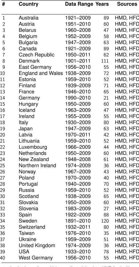
We obtained data on period survival and fertility from the Human Mortality Database (Human Mortality Database 2014), the Human Fertility Database (Human Fertility Database 2014) and the Human Fertility Collection (Human Fertility Collection 2014). These age-specific data were available for 40 developed countries for varying numbers of years (Table 1).
analyzed the ethnic Hutterites of North America, an Anabaptist religious sect with un-regulated fertility reported to have the highest TFR of any known population (Eaton and Mayer 1953). We used Hutterite fertility rates from a study by Eaton and Mayer (1953) covering the period of 1946-1950. We follow Eaton and Mayer in assuming that Hutterite mortality was similar to the overall U.S. rates during this period.
2.3 Characterizing patterns of LRO
The computation of LRO statistics from the available data permits many different compar-isons. We will consider LRO by age, LRO over time, LRO in relation to socio-economic indicators, and the relationship among the different statistics in LRO. Here, we provide more detail of what each of these comparisons entails.
We will present the mean, standard deviation (SD), coefficient of variation (CV), and skewness (Sk) of remaining LRO as a function of age, for a fixed year. Over time, we will show the patterns in mean LRO, standard deviation, coefficient of variation and skewness in LRO at birth for each country. Our focus lies on the period from 1965 to 2010, the period characteristically associated with the second demographic transition. We assess whether our results for LRO are similar to known results using TFR and whether similar patterns arise in the other statistics of LRO.
The relationship between LRO and socio-economic indicators is investigated using the Human Development Index, as LRO presumably responds to the conditions in which individuals find themselves. The HDI, as employed by the United Nations Development Programme, measures a country’s health, education and standard of living. These mea-sures are assigned equal weight and combined into a broad-scale indicator of human development (United Nations Development Programme 2014). Myrskyl¨a, Kohler, and Billari (2009) found a relationship between period TFR and the human development in-dex (HDI). Increases in the HDI up to∼0.9were associated with declines in TFR, but above that point, they found evidence that the TFR began to increase. To evaluate such changes for the mean and variation, we regressed the statistics of LRO for all countries, at age 0, against the HDI for the years 1980 and 2009.
Table 1: Countries used in the analyses
# Country Data Range Years Sources
1 Australia 1921–2009 89 HMD, HFC
2 Austria 1951–2010 60 HMD, HFD
3 Belarus 1960–2008 47 HMD, HFC
4 Belgium 1952–2009 58 HMD, HFC
5 Bulgaria 1947–2009 63 HMD, HFD
6 Canada 1921–2009 89 HMD, HFD
7 Czech Republic 1950–2011 62 HMD, HFD
8 Denmark 1901–2011 111 HMD, HFC
9 East Germany 1956–2010 55 HMD, HFD
10 England and Wales 1938–2009 72 HMD, HFD
11 Estonia 1959–2010 52 HMD, HFD
12 Finland 1939–2009 71 HMD, HFD
13 France 1946–2010 65 HMD, HFD
14 Germany 1990–2010 21 HMD, HFD
15 Hungary 1950–2009 60 HMD, HFD
16 Iceland 1963–2009 47 HMD, HFC
17 Ireland 1955–2009 55 HMD, HFC
18 Italy 1930–2009 80 HMD, HFC
19 Japan 1947–2009 63 HMD, HFD
20 Latvia 1970–2011 42 HMD, HFC
21 Lithuania 1959–2010 52 HMD, HFD
22 Luxembourg 1966–2009 44 HMD, HFC
23 Netherlands 1950–2009 60 HMD, HFD
24 New Zealand 1948–2008 61 HMD, HFC
25 Northern Ireland 1974–2009 36 HMD, HFD
26 Norway 1967–2009 43 HMD, HFD
27 Poland 1970–2009 40 HMD, HFC
28 Portugal 1940–2009 70 HMD, HFD
29 Russia 1959–2010 52 HMD, HFD
30 Scotland 1938–2009 65 HMD, HFD
31 Slovakia 1950–2009 60 HMD, HFD
32 Slovenia 1983–2009 27 HMD, HFD
33 Spain 1922–2009 88 HMD, HFC
34 Sweden 1891–2010 120 HMD, HFD
35 Switzerland 1932–2011 80 HMD, HFD
36 Taiwan 1976–2010 35 HMD, HFD
37 Ukraine 1959–2009 51 HMD, HFD
38 United Kingdom 1974–2009 36 HMD, HFD
39 USA 1933–2010 78 HMD, HFD
40 West Germany 1956–2010 55 HMD, HFD
3. Results
3.1 LRO patterns over age
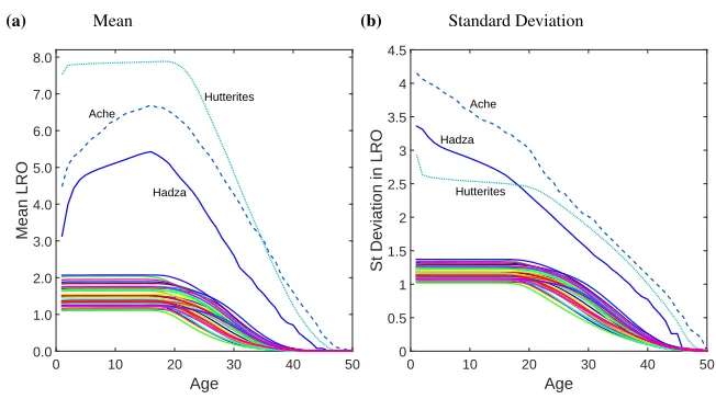
In Figure 1, the mean and standard deviation (SD) of remaining LRO are shown as a function of age. After age 20, all populations show a decline in both mean and SD, until women reach the age of infertility around age 45–50. The Hutterites show a slight increase in mean LRO between age 0 and age 1. In the two hunter-gatherer populations, mean remaining LRO increases with age between birth and age 20. These increases reflect the high infant mortality rates in these populations. The SD of remaining LRO decreases almost linearly with age for the Ache and Hadza.
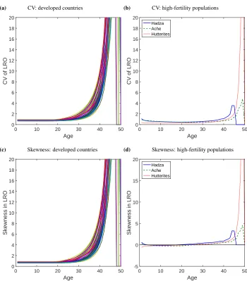
In Figure 2 the coefficient of variation (CV) and skewness (Sk) in remaining LRO are shown separately for developed countries and for the hunter-gatherers and Hutterites. The relative variation in remaining LRO, as measured by the CV, is between 0.5 and 1 at birth for the developed countries, but rises rapidly with age after age 25. The remaining LRO of women over age 40 is extremely variable; by age 45 the CV peaks at values between 40 and a little over 300. Hutterite lifetime CV is the lowest measured, falling just below 0.4. Ache lifetime CV is just below 1, whereas the Hadza are the only population with a CV at birth over 1.
Figure 1: Mean and standard deviation of LRO as a function of age
(a) Mean
Age
0 10 20 30 40 50
Mean LRO
0.0 1.0 2.0 3.0 4.0 5.0 6.0 7.0 8.0
Hadza Ache
Hutterites
(b) Standard Deviation
Age
0 10 20 30 40 50
St Deviation in LRO
0 0.5 1 1.5 2 2.5 3 3.5 4 4.5
Hadza Ache
Hutterites
The skewness of remaining LRO follows a similar pattern. Skewness at birth in the developed countries is slightly positive (between 0.5 and 1) and increases dramatically at older ages. Skewness in LRO at birth is slightly negative for the Hutterites, and remains so until after age 20. For the Hadza and Ache, skewness starts of between 0 and 1, drops to slightly negative values, then becomes positive again around age 20. Hadza and Ache women show lower peaks in CV and skewness around age 45, whereas Hutterites show variability comparable to developed countries at this age.
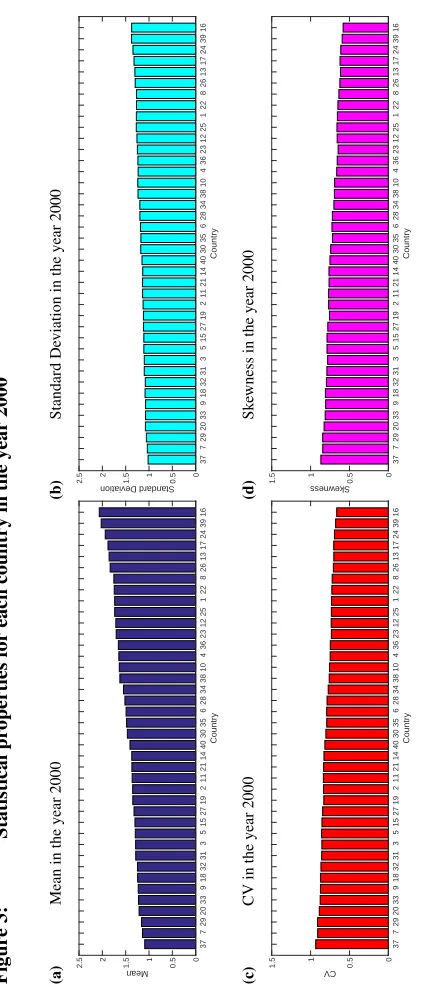
In Figure 3, the lifetime values for mean, standard deviation, CV and skewness of LRO at birth are shown for all 40 countries in the year 2000, corresponding to the values in the age-dependent graphs at age 0. Mean LRO was below replacement (2.1) in 2000 for all countries.
3.2 Patterns over time
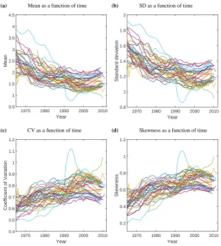
We focus on the period during which most developed countries experienced the second demographic transition (1965-2010). Our results for mean LRO agree with other well-known results concerning the transition: LRO declines sharply and then begins to rise again in recent years (Goldstein, Sobotka, and Jasilioniene 2009; Myrskyl¨a, Kohler, and Billari 2009). Measures of variability, however, display different patterns. The standard deviation of LRO also declines sharply from 1965 to about 2000, and shows signs of beginning to recover from 2000–2010. The coefficient of variation increases from 1965, levelling off after 2000. The skewness does the same, showing a very similar pattern to the CV.5
The magnitude of increase or decrease in statistical properties of LRO differs be-tween different countries. Moreover, not all countries show a reversal in pattern in the last 5-10 years. The time series for mean and standard deviation appear similar for all countries, and also inversely similar to CV and skewness.
We have included a gallery showing the time series of the statistics of LRO at se-lected ages, for all 40 developed countries, in an Online Supplement.
3.3 Relationship to HDI
The HDI is a synthetic index designed to describe socioeconomic living conditons. The decline in TFR during the transition has been associated with improvement in standards of living. Myrskyl¨a, Kohler, and Billari (2009) found that TFR declined with increases in the HDI up to a point, but that further increases in the HDI were associated with increases in TFR.
5The similarity of values of the coefficient of variation and of skewness was noted in several species by Caswell
Figure 2: CV and skewness of LRO as a function of age
(a) CV: developed countries
Age
0 10 20 30 40 50
CV of LRO
0 2 4 6 8 10 12 14 16 18 20
(b) CV: high-fertility populations
Age
0 10 20 30 40 50
CV of LRO
0 2 4 6 8 10 12 14 16 18 20
Hadza Ache Hutterites
(c) Skewness: developed countries
Age
0 10 20 30 40 50
Skewness in LRO
0 2 4 6 8 10 12 14 16 18 20
(d) Skewness: high-fertility populations
Age
0 10 20 30 40 50
Skewness in LRO
-5 0 5 10 15 20
Hadza Ache Hutterites
Notes: Coefficient of variation and skewness of age-specific remaining lifetime reproductive output for 40 developed
countries in the year 2000 ((a),(c)), as well as for two hunter-gatherer populations, namely the Ache (dashed
Figure 4: Statistical properties of LRO across the second demographic transition
(a) Mean as a function of time
Year
1970 1980 1990 2000 2010
Mean
0.5 1 1.5 2 2.5 3 3.5 4 4.5
(b) SD as a function of time
Year
1970 1980 1990 2000 2010
Standard deviation
0.8 1 1.2 1.4 1.6 1.8 2
(c) CV as a function of time
Year
1970 1980 1990 2000 2010
Coefficient of Variation
0.4 0.5 0.6 0.7 0.8 0.9 1 1.1 1.2
(d) Skewness as a function of time
Year
1970 1980 1990 2000 2010
Skewness
0.2 0.4 0.6 0.8 1 1.2
Notes: Mean(a), standard deviation(b), CV(c)and skewness(d)of lifetime reproduction during the period of the second demographic transition for 40 developed countries. The light blue line is East Germany; reasons for its unusual trajectory have been discussed by Witte and Wagner (1995) and Adler (1997).
Kohler, and Billari (2009), we find a negative relationship between mean LRO and HDI in the year 1980, but a positive relationship in the year 2009 (see Figure 5(a)). Further-more, we find a similar reversal in the relationship between HDI and the other statistical properties of LRO (see Figure 5(b-d)). The standard deviation decreased with HDI in the 1980, but increased with HDI in 2009. The CV and skewness show opposite patterns to mean and SD, as both increased with HDI in 1980 and decreased with HDI in 2009. In earlier years, with lower values of HDI, improvements in economic and living conditions led to reduced mean LRO and SD, but increased relative variability as measured by the CV and increased skewness. In later years, the slopes are reversed (see Table A1 for the regression line equations).
Figure 5: Relationship between statistical properties of LRO and HDI
(a) Mean as a function of HDI
0.6 0.7 0.8 0.9 1.0
1.0
1.5
2.0
2.5
HDI
Mean
1980 2009
(b) SD as a function of HDI
0.6 0.7 0.8 0.9 1.0
1.0
1.2
1.4
1.6
HDI
Standard De
viation
1980 2009
(c) CV as a function of HDI
0.6 0.7 0.8 0.9 1.0
0.5
0.7
0.9
HDI
CV
1980 2009
(d) Skewness as a function of HDI
0.6 0.7 0.8 0.9 1.0
0.5
0.7
0.9
HDI
Sk
e
wness
1980 2009
3.4 Relationships among the statistics of LRO
The mean, variance, coefficient of variation, and skewness provide a statistical character-ization of the LRO implied by the life table and the fertility schedule. When compared across developed countries, a general relationship between these statistics exists. The scatterplot in Figure 6 shows the relationships among all statistics for all countries in the year 2000. The mean and standard deviation of LRO are positively related to each other, as are CV and skewness. The former statistics are, however, negatively related to the latter (see Table A2 for regression line equations).
When we added data from two additional years (1990 and 2005), the statistics of LRO became slightly less tightly distributed (van Daalen and Caswell, unpublished data). To further explore changes over time, we created phase portraits showing the dynamics of the mean and SD over the historical records available for the countries. Figure 7 shows the time trajectories for 4 countries (Bulgaria, Canada, Japan, and Sweden). The dotted line in the figures is the regression line relating the mean and SD in the scatterplot in Figure 6.
In all four countries, the mean and SD of lifetime reproduction converge to the inter-country regression line. Before the convergence statistics of LRO were more variable both within and between countries. After this convergence countries moved along the line, with both the mean and SD declining at first, before increasing again, as is also shown in Figure 4. The fact that the countries practically “retrace their steps” along the line reinforces the idea of the existence of a universal distribution of LRO to which developed countries appear to converge. Similar patterns were found in all 40 countries we examined.
4. Discussion
Figure 7: Time trajectories of mean and standard deviation of LRO
(a) Bulgaria
Mean
1 1.5 2 2.5
Standard deviation
1 1.1 1.2 1.3 1.4 1.5 1.6 1.7 1.8 1.9
1947
2009
(b) Canada
Mean
1 1.5 2 2.5 3 3.5 4
Standard deviation
1 1.2 1.4 1.6 1.8 2 2.2
1921
2009
(c) Japan
Mean
1 1.5 2 2.5 3 3.5 4
Standard deviation
1 1.5 2 2.5
1947
2009
(d) Sweden
Mean
1 1.5 2 2.5 3
Standard deviation
1 1.2 1.4 1.6 1.8 2 2.2 2.4 2.6
1891
2010
Notes: Trajectories of the mean plotted against standard deviation over time. The starting and ending years are indicated for each trajectory. The dotted lines represent the regression line through the scatterplot of mean and SD shown in Figure 6.
the other moments change along with it. Therefore, during the second demographic tran-sition, not only mean LRO, but the entire distribution of lifetime reproductive output changed. The transition was characterized by a decreasing mean lifetime reproductive output, a decreasing standard deviation (so a decreasing spread in values), an increas-ing CV (i.e. an increase in the measure of relative variation) and an increasincreas-ing, positive skewness (an increase in the degree of asymmetry characterizing the distribution).
The tight link between statistical properties of LRO across different developed coun-tries in the year 2000 (Figure 6) suggests a universal distribution of LRO. If mortality were so low that all individuals survived through their reproductive years, then LRO would be the sum of 50 Bernoulli trials, with a different probability at each age. Such a sum is a random variable with a Poisson-binomial distribution. If the probabilities are small enough, the Poisson-binomial distribution is well approximated by the Poisson distribu-tion (Le Cam 1960; Steele 1994).
The mean and variance of the Poisson distribution are equal, the coefficient of vari-ation is a function of the mean, and the coefficient of varivari-ation and skewness are equal. We observe these relationships to some extent in Figure 6 when mortality has become very low in these countries. In earlier years, or in the fixed reward model, the relation-ships among the statistics of LRO are much looser (van Daalen and Caswell, unpublished data).
4.1 Individual stochasticity and its components
Individual variation has received considerable attention in studies of mortality, but very little in studies of fertility. There is a large literature examining patterns of variation in the age at death and a variety of indices of discrepancy in longevity (Anand and Nanthikesan 2000; van Raalte and Caswell 2013). Like all life table calculations, these assume that all individuals experience the same set of specified vital rates, and hence the calculated variation is due to individual stochasticity (van Raalte and Caswell 2013). Studies of fer-tility have paid much less attention to inter-individual variation of lifetime reproduction. Instead, focus has been largely on expectations of various kinds (R0or TFR) and how
those expectations change. Our results here are, to our knowledge, the first comparative study of the inter-individual variation in LRO implied by mortality and fertility schedules. The variance in LRO due to individual stochasticity comes from two sources. Indi-viduals may follow different pathways through life; this variation is generated from the transition matrixUin equation (1). In the simple age-classified case considered here, the pathway taken by an individual is completely specified by its age at death.6 The other
component of variance comes from the stochastic nature of reproduction at each age,
6In more complex or multi-state models, pathways can be more varied; see, e.g., the age×parity model of
which enters the model through the matricesRigiving the moments of the reproductive “rewards” in equations (4) and (5).
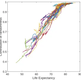
Mortality rates have declined, and life expectancies increased, during the demo-graphic transition. As a result, the chance that a woman will survive to the end of her reproductive years has increased; hence we expect more and more of the variance in LRO to be accounted for by the stochastic nature of reproduction. To evaluate this, we compare the variance from the full model with the results of a model in which the fertility rewards are fixed, rather than stochastic. In a fixed reward model (Caswell 2011) a fertility of fi implies that every individual of ageiproduces a fraction fi of a child, rather than producing one or zero children with probabilitiesfiand1−fi.
Figure 8 shows the fraction of the variance in LRO due to the variance in the fertility rewards, as a function of life expectancy, for the developed countries in our dataset. As life expectancy increases, the proportion of variance explained by the randomness in the rewards approaches 1. We conclude that improvement of health and life expectancy, and the subsequent reduction of the influence of mortality, plays a crucial role in determining the distribution of lifetime reproduction in developed countries.
4.2 Individual stochasticity
The inter-individual variation in LRO shown here is a function of individual stochasticity alone. Our results do not incorporate heterogeneity among individuals in mortality or fertility. They could be interpreted as baseline results in comparison to measurements of actual lifetime reproduction (Caswell 2011; Steiner and Tuljapurkar 2012). Adding fur-ther dimensions of heterogeneity in addition to age may increase or decrease the variance in LRO (Caswell 2014b). The overall effect of heterogeneity on LRO is an open prob-lem; distinguishing the two effects will require models that incorporate heterogeneity, as frailty models do for studies of mortality.
18th and 19th century are different from those of Europe during the second demographic transition, but this crude comparison suggests that the opportunity for selection is to a large part determined by heterogeneity, with only a relatively small contribution from individual stochasticity. Such comparisons are a valuable tool for understanding observed variance in LRO (Tuljapurkar, Steiner, and Orzack 2009; Steiner and Tuljapurkar 2012; van Daalen and Caswell 2015).
Figure 8: Partitioning the variance in LRO as a function of life expectancy
Life Expectancy
40 50 60 70 80 90
Contribution of randomness
0.3 0.4 0.5 0.6 0.7 0.8 0.9 1
will show how the statistics of LRO respond to changes in the parameters of the mortality and fertility schedules (Caswell and van Daalen 2015). Finally, we note that the method can be applied to rewards other than reproductive output, including health and longevity (Caswell and Zarulli, unpublished data) and lifetime accumulation of economic rewards (Caswell and Kluge 2015).
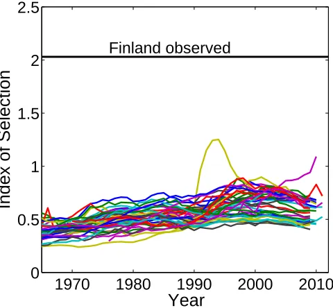
Figure 9: Standardized variance due to individual stochasticity compared to observed value for Finland 1760–1849
1970
1980
1990
2000
2010
0
0.5
1
1.5
2
2.5
Finland observed
Index of Selection
Year
Notes: The standardized variance (Crow’s index of selection) for 40 developed countries during the second demo-graphic transition, compared to the standardized variance of LRO among women in Finland living between 1760 and 1849 (Courtiol et al. 2012).
5. Acknowledgements
References
Adler, M.A. (1997). Social change and declines in marriage and fertility in eastern Ger-many.Journal of Marriage and Family59(1): 37–49. doi:10.2307/353660.
Anand, S. and Nanthikesan, S. (2000). A compilation of length-of-life distribution mea-sures for complete life tables. Working Paper (10) 7, Harvard Center for Population and Development Studies, Harvard School of Public Health.
Blurton Jones, N. (2011). Hadza demography and sociobiology. Retrieved from http://www.sscnet.ucla.edu/anthro/faculty/blurton-jones/hadza-part-1.pdf.
Bongaarts, J. and Sobotka, T. (2012). A demographic explanation for the recent rise in European fertility. Population and Development Review 38(1): 83–120.
doi:10.1111/j.1728-4457.2012.00473.x.
Breuer, T., Robbins, A.M., Olejniczak, C., Parnell, R.J., Stokes, E.J., and Robbins, M.M. (2010). Variance in the male reproductive success of western gorillas: Acquiring fe-males is just the beginning. Behavioural Ecology and Sociobiology64(4): 515–528.
doi:10.1007/s00265-009-0867-6.
Brown, D. (1988). Components of lifetime reproductive success. In: Clutton-Brock, T.H. (ed.).Reproductive Success. Chicago: University of Chicago Press: 439–453.
Bryant, J. (2007). Theories of fertility decline and the evidence from development in-dicators. Population and Development Review33(1): 101–127. doi:10.1111/j.1728-4457.2007.00160.x.
Caswell, H. (2001). Matrix Population Models: Construction, Analysis, and Interpreta-tion. Sunderland: Sinauer Associates, 2nd ed.
Caswell, H. (2006). Applications of Markov chains in demography. In: MAM2006: Markov Anniversary Meeting.Raleigh, North Carolina: Boson Books, 319–334. Caswell, H. (2009). Stage, age and individual stochasticity in demography. Oikos118:
1763–1782.doi:10.1111/j.1600-0706.2009.17620.x.
Caswell, H. (2011). BeyondR0: Demographic models for variability of lifetime
repro-ductive output.PLoS ONE6(6): e20809.doi:10.1371/journal.pone.0020809.
Caswell, H. (2014a). A matrix approach to the statistics of longevity in heterogeneous frailty models. Demographic Research 31: 553–592.
doi:10.4054/DemRes.2014.31.19.
Caswell, H. and Kluge, F.A. (2015). Demography and the statistics of lifetime eco-nomic transfers under individual stochasticity. Demographic Research32: 563–588.
doi:10.4054/DemRes.2015.32.19.
Caswell, H. and van Daalen, S.F. (2015). Markov chains with random rewards: Equilibria and sensitivity of long-term accumulation. Preprint.
Clutton-Brock, T.H. (1988). Reproductive Success. Chicago: University of Chicago Press.
Courtiol, A., Pettay, J.E., Jokela, M., Rotkirch, A., and Lummaa, V. (2012). Natural and sexual selection in a monogamous historical human population. Proceedings of the National Academy of Sciences109(21): 8044–8049. doi:10.1073/pnas.1118174109. Crow, J.F. (1958). Some possibilities for measuring selection intensities in man. Human
Biology30(1): 1–13.
Cushing, J. and Zhou, Y. (1994). The net reproductive value and stability in matrix population models.Natural Resources Modeling8(4): 297–333.
Eaton, J.W. and Mayer, A.J. (1953). The social biology of very high fertility among the Hutterites: The demography of a unique population.Human Biology25(3): 206–264. Feichtinger, G. (1973). Markovian models for some demographic processes.Statistische
Hefte14: 310–334.doi:10.1007/BF02923066.
Goldstein, J.R., Sobotka, T., and Jasilioniene, A. (2009). The end of “lowest-low” fer-tility? Population and Development Review 35(4): 663–699. doi:10.1111/j.1728-4457.2009.00304.x.
Grafen, A. (1988). On the uses of data on lifetime reproductive success. In: Clutton-Brock, T.H. (ed.).Reproductive Success. Chicago: University of Chicago Press: 454– 471.
Gurven, M. and Kaplan, H. (2007). Longevity among hunter-gatherers: A cross-cultural examination. Population and Development Review 33(2): 321–365.
doi:10.1111/j.1728-4457.2007.00171.x.
Heesterbeek, J.A. (2002). A brief history of R0 and a recipe for its calculation. Acta Biotheoretica50(3): 189–204. doi:10.1023/A:1016599411804.
Hill, K. and Hurtado, A. (1996). Ach´e Life History: The Ecology and Demography of a Foraging People. Evolutionary Foundations of Human Behavior Series. New York: Aldine de Gruyter.
doi:10.1146/annurev.anthro.28.1.397.
Howard, R.A. (1960). Dynamic Programming and Markov Processes. New York: Tech-nology Press and Wiley.
Human Fertility Collection (2014). Max Planck Institute for Demographic Re-search (Germany) and the Vienna Institute of Demography (Austria). URL www. fertilitydata.org.
Human Fertility Database (2014). Max Planck Institute for Demographic Re-search (Germany) and the Vienna Institute of Demography (Austria). URL www. humanfertility.org.
Human Mortality Database (2014). University of California, Berkeley (USA), and Max Planck Institute for Demographic Research (Germany). URL www.mortality. org.
Kirk, D. (1996). Demographic transition theory. Population Studies50(3): 361–387.
doi:10.1080/0032472031000149536.
Le Bras, H. (2008). The Nature of Demography. Princeton, NJ: Princeton University Press.
Le Cam, L. (1960). An approximation theorem for the Poisson binomial distribution. Pacific Journal of Mathematics10(4): 1181–1197. doi:10.2140/pjm.1960.10.1181. Lee, R. (2003). The demographic transition: Three centuries of
fun-damental change. Journal of Economic Perspectives 17(4): 167–190.
doi:10.1257/089533003772034943.
Liu, J., Rotkirch, A., and Lummaa, V. (2012). Maternal risk of breeding failure remained low throughout the demographic transitions in fertility and age at first reproduction in Finland. PLoS ONE7(4): e34898. doi:10.1371/journal.pone.0034898.
Lotka, A.J. (1936). The geographic distribution of intrinsic natural increase in the United States, and an examination of the relation between several measures of net reproductivity. Journal of the American Statistical Association 31: 273–294.
doi:10.1080/01621459.1936.10503330.
Myrskyl¨a, M., Kohler, H.P., and Billari, F.C. (2009). Advances in development reverse fertility declines. Nature460(7256): 741–743. doi:10.1038/nature08230.
Newton, I. (1989). Lifetime reproduction in birds. New York: Academic Press.
103: 61–89. doi:10.2307/2980551.
Robbins, A.M., Stoinski, T., Fawcett, K., and Robbins, M.M. (2011). Lifetime reproduc-tive success of female mountain gorillas. American Journal of Physical Anthropology 146(4): 582–593.doi:10.1002/ajpa.21605.
Spuhler, J.N. (1976). The maximum opportunity for natural selection in some human populations. In: Zubrow, E.B.W. (ed.).Demographic Anthropology: Quantitative Ap-proaches. Albuquerque, New Mexico: University of New Mexico Press: 185–226.
Steele, J.M. (1994). Le Cam’s inequality and Poisson approximations.American Mathe-matical Monthly101(1): 48–54.doi:10.2307/2325124.
Steiner, U.K. and Tuljapurkar, S. (2012). Neutral theory for life histories and individual variability in fitness components. Proceedings of the National Academy of Sciences 109(12): 4684–4689.doi:10.1073/pnas.1018096109.
Tuljapurkar, S., Steiner, U.K., and Orzack, S.H. (2009). Dynamic heterogeneity in life histories. Ecology Letters12: 93–106. doi:10.1111/j.1461-0248.2008.01262.x. United Nations Development Programme (2014). Human Development Index
(HDI). Retrieved from http://hdr.undp.org/en/content/human-development-index-hdi, 1 April 2014.
van Daalen, S. and Caswell, H. (2015). Lifetime reproductive output in birds and mam-mals.(in prep.).
van Raalte, A.A. and Caswell, H. (2013). Perturbation analysis of indices of lifespan variability.Demography50(5): 1615–1640.doi:10.1007/s13524-013-0223-3. Vaupel, J.W., Manton, K.G., and Stallard, E. (1979). The impact of heterogeneity
in individual frailty on the dynamics of mortality. Demography 16(3): 439–454.
doi:10.2307/2061224.
Wilson, C. (2004). Fertility below replacement level. Science 304(5668): 207–209.
doi:10.1126/science.304.5668.207c.
Witte, J.C. and Wagner, G.G. (1995). Declining fertility in East Germany after unifica-tion: A demographic response to socioeconomic change.Population and Development Review21(2): 387–397. doi:10.2307/2137500.
Woofter, T. (1949). The relation of the net reproduction rate to other fertil-ity measures. Journal of the American Statistical Association 44: 501–517.
1. Appendix
In Table A1, equations are shown for the regression of several statistics of LRO as func-tions of HDI. These lines, for the year 1980 and the year 2009, are drawn in Figure 5 as well. Table A2 shows the regression lines for the relationships among the statistical properties of LRO.
Table A1: Regression lines for the statistics of LRO as functions of HDI
Statistic 1980 2009
Mean 3.054−0.578×HDI −0.312 + 2.239×HDI
Standard Deviation 1.775−0.616×HDI 0.611 + 0.710×HDI
CV 0.517 + 0.262×HDI 1.247−0.558×HDI
Skewness 0.293 + 0.423×HDI 1.240−0.634×HDI