ENERGY-EFFICIENT FAULT TOLERANT COVERAGE FOR WIRELESS SENSOR NETWORKS

(1)

FOR WIRELESS SENSOR NETWORKS

by

Rahul Kavalapara

A thesis

submitted in partial fulfillment of the requirements for the degree of Master of Science in Computer Science

Boise State University

(2)

DEFENSE COMMITTEE AND FINAL READING APPROVALS

of the thesis submitted by

Rahul Kavalapara

Thesis Title: Energy-Efficient Fault Tolerant Coverage For Wireless Sensor Networks

Date of Final Oral Examination: 01 August 2010

The following individuals read and discussed the thesis submitted by student Rahul Kavala-para, and they evaluated his presentation and response to questions during the final oral examination. They found that the student passed the final oral examination.

Sirisha Medidi, Ph.D. Chair, Supervisory Committee

Murali Medidi, Ph.D. Member, Supervisory Committee

Jyh-haw Yeh, Ph.D. Member, Supervisory Committee

(3)

I would like to express my deepest gratitude to my advisor, Dr. Sirisha, for her guidance and inspiration. Her insights have strengthened this study significantly. I will always be thankful for her wisdom, knowledge, and deep concern.

My sincere thanks to Dr. Murali for being on my thesis committee. His lectures were very inspirational and have changed the way I think today.

I thank Dr. Yeh for his inputs and for serving as a committee member and for evaluating my thesis.

My thanks to fellow grad students at SWAN Lab for their support.

Special thanks to my parents for their love and support and providing me an opportunity to pursue a masters program, and to Rajeev and Shriya.

(4)

Wireless Sensor Networks are generally deployed in harsh environments to perform sensing operations and communication between sensors to report the events in applications like military surveillance, environmental monitoring, and etc. Sensor networks are resource constrained and the tiny size of sensors limits transmission power, bandwidth, and memory space. Errors in sensor networks such as noise interference, signal fading, and terrain pose a challenge in detecting and reporting events. Events undetected or not reported reduce the quality of any coverage protocol. As sensors are battery operated and energy constrained, there is also a need to maintain energy efficiency of the network. Current coverage protocols only focus on the entire area being covered but not event reporting and energy efficiency. To ensure that a better quality of service is provided by coverage pro-tocols, there is a need for providing fault tolerance and event reporting while maintaining energy efficiency of the network. This thesis proposes a fault tolerant coverage protocol that enhances event reporting with the help of additional support structure and energy efficiency by reducing the communication. To further reduce the energy consumption and congestion in the network, only a subset of nodes are chosen to perform sensing and communication. We implemented our coverage protocol using the ns2 simulator for evaluating its performance. Simulation results show that our protocol has better event reporting and energy savings.

(5)

ABSTRACT . . . iv

LIST OF TABLES . . . vii

LIST OF FIGURES . . . viii

1 Introduction . . . 1

1.1 Outline of Thesis . . . 4

2 Related Work . . . 5

2.1 Classification of Coverage . . . 5

2.1.1 Fault Tolerance . . . 7

2.1.2 Sensing and Transmission Radii . . . 12

2.1.3 Deployment Strategies . . . 15

2.2 Energy Efficient Coverage . . . 16

2.3 Event Transfer Protocols . . . 18

3 Fault Tolerant Coverage . . . 22

3.1 Motivation and Design Requirements . . . 22

3.2 Backup Coverage . . . 27

3.2.1 2 - Coverage . . . 29

3.2.2 Voronoi Diagrams and Delaunay Triangulation . . . 31

3.2.3 Selection of Backup Nodes . . . 33

(6)

3.3.1 Event Detection . . . 36

3.3.2 Backup Reporting . . . 37

3.4 Event Reporting . . . 39

4 Performance Evaluation . . . 42

4.1 Fault Tolerance . . . 42

4.3 Energy Efficiency . . . 52

5 Conclusions . . . 55

REFERENCES . . . 57

(7)

4.1 Parameters for Low Power . . . 43 4.2 Parameters for High Power . . . 43

(8)

2.1 Target Coverage . . . 6

2.2 Area Coverage . . . 7

2.3 Sensing Radii in WSN . . . 12

3.1 Subsetting of Nodes . . . 29

3.2 Voronoi Diagram and Delaunay Triangulation of a Random Topology . . . 32

3.3 Selection of Backup Nodes from Double Coverage Set . . . 34

3.4 Backup Functionality . . . 36

3.6 Spatially correlated contention . . . 41

4.1 Active Node Count vs Number of Nodes Deployed . . . 43

4.2 Coverage Ratio vs Number of Nodes Deployed . . . 45

4.3 Number of Events Detected vs Percentage Node Failure . . . 46

4.4 Events Reported (High Load) vs Percentage Node Failure . . . 48

4.5 Events Reported (Medium Load) vs Percentage Node Failure . . . 49

4.6 Events Reported (Low Load) vs Percentage Node Failure . . . 50

4.7 Energy Consumed (High Load) vs Number of Nodes . . . 52

4.8 Energy Consumed (Medium Load) vs Number of Nodes . . . 52

4.9 Energy Consumed (Low Load) vs Number of Nodes . . . 53

(9)

CHAPTER 1 INTRODUCTION

Wireless Sensor Networks (WSNs) consists of a large number of tiny sensors used for monitoring, communication, and computational purposes. Sensor nodes are self-governing entities that collaborate with each other to perform sensing operations. Their features of self-organization and dynamic reconfiguration make them a perfect choice for applications to monitor and gather physical data in harsh environments. Sensor nodes provide absolute results in monitoring the region of interest. They prove to be a feasible solution in com-parison with other conventional networks, where deployment of conventional networks is impractical. To illustrate a few applications, WSNs are deployed in the following: military surveillance, environmental monitoring, air/water quality, and etc. The tiny size and mobile characteristics of sensor nodes are added benefits as they can be easily deployed to monitor any given region.

(10)

amount of communication, distributed/local pre-computation techniques, complex power saving modes, and large scale networks. Because sensor networks are energy constrained, the primary goal is to maintain energy efficiency of the network.

There are several other problems associated with energy efficiency that play a major role in achieving the goals of a deployed sensor network. One such critical problem is coverage. Coverage can be described as how well the geographical region is monitored.

Coverage can also be defined as the quality of service provided by a sensor network. In sensor networks, coverage is classified in several ways based on different criteria. Area coverage is one of the classifications. Other classifications of coverage are presented in Chapter 2. Area coverage deals with the entire geographical region being monitored, and that every location in the region is monitored by at least one sensor node. Each node monitors an area of geographical region within its boundary, also known as the sensing region and the distance from the node to the boundary is known as the sensing radius. It is essential for a wireless sensor network to monitor every location in the region to provide sensing information, proving the importance of coverage in a sensor network. All locations in geographical region are 1-covered when each location in the region is within the sensing range of at least one sensor node.

(11)

and K-coverage assists in handling the problem as neighboring nodes provide additional advantage of detection when a node fails to detect the event due to errors in the network.

Current coverage mechanisms proposed so far do not facilitate fault tolerance and energy efficiency together. Sensor networks are energy constrained as they are battery operated, but in addition to providing fault tolerant coverage, the energy efficiency of the network must be maintained. K-coverage mechanisms proposed in the literature are not energy efficient as several sensors report simultaneously, leading to excessive energy consumption, congestion, and collisions in the network. This reduces the quality of service and network performance.

Coverage mechanisms introduced previously only meet the requirement of sensors cov-ering the region of interest within the sensing region of sensor nodes. Current techniques proposed to date have addressed the issue of the area being constantly covered. However, these techniques have failed to address the quality of service in sensor networks. To provide quality of service in monitoring a given region, with the region completely covered, sensors must also detect the events occurring in the region and report them. For improving the quality of service provided by the coverage mechanisms, there is a need for coverage techniques that ensure event detection and reporting.

This thesis addresses the issue of improving the quality of service by providing fault tolerance, event reporting, and energy efficiency in coverage. With the help of Backup nodes, which are selected to support existing 1-coverage, a backup structure is provided

(12)

1.1 Outline of Thesis

(13)

CHAPTER 2 RELATED WORK

The problem of coverage exists in several domains of research. One of the well-known visibility problems, known as theArt Gallery problem, deals with finding the number of observers required such that each and every point in a room is covered by at least one observer. Several applications have originated from this problem. These include finding a minimum set of sensors to monitor a given region and optimizing the number of cell phone towers to be placed in an area for wireless communication. Coverage in WSN is similar to the art gallery problem with a different set of constraints and semantics. In WSNs, the coverage problem was initially reviewed as an area coverage problem. As wireless sensor networks are resource constrained, and to provide quality monitoring services, energy effi-ciency and event reporting play a very important role and contribute to coverage protocols in WSNs. Many protocols have been proposed to provide coverage, energy efficiency, and reliable event transfer in WSN research. These approaches will be discussed in detail in further sections.

2.1 Classification of Coverage

(14)

T2

T1 T3

T4 S1

S2 S3

Figure 2.1: Target Coverage in Wireless Sensor Networks

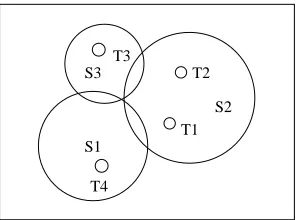
Target Coverage: In target coverage, objects/targets are essentially monitored in a given region of deployment. The complexity of target coverage multiplies with an increase in number and mobility of targets. Target coverage is illustrated in Figure 2.1, whereS1, S2 andS3are sensors monitoring targetsT1, T2, T3 andT4. Many target coverage protocols are approached in different ways. These protocols can be referred to in detail in [4, 7, 10, 26, 56, 57].

(15)

1− Coverage

3 − Coverage 2 − Coverage

A B

C

Figure 2.2: Area Coverage

preference for selection in the set cover to provide coverage. Selection of the sensor node into a set cover is repeated to maintain target coverage all the time. The goal of [5] is to increase the network lifetime and reduce the energy consumption in addition to providing target coverage. However, the energy consumed by the sensor nodes is not presented.

Area Coverage: In sensor networks, area coverage is one of the most researched areas in coverage problems. Area coverage problems are not limited to sensor networks, but its applications range from ad hoc wireless networks and other areas to computational geometry. Area coverage deals in monitoring the entire physical space of interest with the set of deployed sensor nodes. In this thesis, the research is mainly associated with area coverage in sensor networks.

2.1.1 Fault Tolerance

(16)

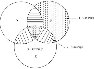
detection. Fault tolerant sensor networks have higher a coverage degree to handle the chal-lenges in WSN. The coverage degree of a sensor network can be defined as the minimum sensors monitoring every location in a given region. Figure 2.2 illustrates, area covered by senor nodes and represented with dashed lines has coverage degree one, common region covered between two nodes and represented with straight lines has coverage degree two and finally the region within three nodes and represented as a mesh has coverage degree three. The representations are also shown mathematically below.

1 - coverage —- A∪B - ( (A∩B)∪(B∩C) ) 2 - coverage —- A∩B - ( (A∩C)∩(B∩C) ) 3 - coverage —- (A∩C)∩(B∩C)

1 - Coverage: In a given geographical region R, with a set of sensors deployed, the entire area is 1 - covered when every location/target in the geographical region is within the sensing region of at least one sensor node. Sensors providing 1-coverage can be deployed in applications where the requirements are not very critical. Several coverage protocols are proposed to provide 1 - coverage for a given region.

(17)

search techniques based on the breach weight. Breach weight is the distance between the closest sensors present between the start and end locations of the Breach path. With the help of Breach path, additional sensors are deployed around the lower observability areas and coverage is improved. In a similar way to Breach path, the maximum support path is also formed using Delaunay triangulation and binary search techniques with the help of support weight, which is calculated based on the distances closest to the sensor. In the proposed approaches, the Breach and Support path formed are not unique. A centralized commu-nication is assumed and the nodes report to the base station directly, thereby increasing energy consumption in the network.

Other approaches providing 1 - coverage include centralized and distributed greedy heuristics, grid-based techniques and can be found in [18, 19, 22, 24, 27, 35, 38, 40].

K - Coverage: A given region is 2-covered if every point in the geographical region is within the sensing region of at least two sensor nodes. This can be generalized to K-coverage, where the given geographical region is within the sensing region of K dis-tinct sensors. Applications that are very critical and require more fault tolerance need to have K-coverage. Dense deployments having more redundancy are required to provide K-coverage. Sensor networks that are over-provisioned (i.e networks are deployed with

more resources) usek-coverage mechanisms to provide fault tolerance. Several approaches have been proposed to provide K-coverage.

K-coverage is another technique that was proposed initially in [29] to provide better

(18)

K-cover problem. FormingK disjoint covers from the entire collection of deployed sensor nodes is proved to be NP-hard. To solve the setK-cover problem, a heuristic is provided such that the area is Kcovered. The heuristic is based on the maximally constrained -minimally constraining paradigm. The proposed heuristic approach minimizes the cover-age of sparsely covered areas within one set cover using the critical element. The critical element is the sensor node in the set of sensors deployed and is a member of a minimal number of set covers. The set covers are chosen based upon an objective function for each critical element. The heuristic performance is evaluated based on the number of sensor covers formed for the number of sensor nodes deployed and is compared with a simulated annealing approach. The proposed approach tries to maximize the number of set covers being chosen to provide K-coverage. With more set covers being formed, one set being active at any instance of time reduces the energy consumed and also providesK-coverage. The proposed approach does not guarantee every location in the entire region is monitored with same degree ofK-coverage. The percentage of area covered and energy consumed by the sensors in the network are not presented with the heuristic approach.

(19)

sensors is set toOnstate. This process continues until all sensors are chosen to be in On orOff state. Wang et al. extend [46] and propose Coverage Configuration protocol (CCP) to provideK-coverage. In their approach, a node gathers information from its neighboring sensor nodes and decides if the region covered by itself is being monitored byK-different neighboring nodes and has reached the coverage degree K. In their approach, the nodes exist in three different states: Active, Listen,andSleep. They try to minimize the number of nodes by making the node inactive if the region covered by the node is K-covered by its neighbors. The nodes maintain coverage and connectivity by broadcasting ‘hello’ messages to the neighboring nodes. The authors measured and compared between attained and desired coverage degree. The authors also compared their approaches with the Ottawa protocol and SPAN protocols.

(20)

(a) Fixed Radii (b) Variable Radii

Figure 2.3: Sensing Radii in WSN

Several related techniques including randomization, Voronoi diagrams, and others, are also proposed in [12, 25, 28, 42, 53].

2.1.2 Sensing and Transmission Radii

Based on the properties of the sensing and transmission radii of sensors deployed, coverage problem can be classified into coverage using fixed/variable sensing or transmission radii. Coverage based on sensing and transmission radii can be illustrated from Figure 2.3.

Fixed Sensing and Transmission Radii: Sensors possessing the same sensing and trans-mission radii and not having the ability to vary its sensing or transtrans-mission radii, can be mentioned as sensors monitoring the region with fixed sensing and transmission radii. In this thesis, all the sensors are considered possessing a fixed sensing and transmission radii.

(21)

sensors from a given set of deployed sensors in a region by sending Candidate path search (CPS) and Candidate path response (CPR) messages and identifying which nodes provide the greatest benefit and form a connected graph. Nodes with the greatest benefit are the nodes that cover the maximum uncovered region. In their problem formulation, they tried to achieve the entire region being monitored by the candidate set of sensors, and formed a connected graph. All the sensors in the candidate set form a connected graph if each and every sensor in the set is able to communicate or transmit messages to its neighbors within the transmission range of the sensor. The energy consumption of sensor nodes in the network is not presented.

(22)

communica-tion is mainly performed between the sensor and the cluster head.

Variable Sensing and Transmission Radii: Sensors having the ability to vary their sensing radii to provide coverage for a given region can be mentioned as sensors monitoring the region with variable sensing radii. This can be observed from Figure 2.3(b).

Wang and Medidi [39] proposed an energy efficient variable sensing based technique to provide coverage. Delaunay triangulation and Voronoi diagrams as techniques are used to improve the coverage. To improve coverage and provide energy efficiency, distributed heuristics and energy balancing techniques are provided. The region being monitored is ini-tially triangulated using the local Delaunay triangulation one-hop approximation algorithm. The correctness of the one-hop approximation algorithm providing coverage is presented based on the relationship of the transmission and sensing radius. The transmission radius is assumed to be at least twice the sensing radius and the euclidean distance between two adjacent nodes in the triangulation lesser than the transmission radius of the sensor node is used to prove that the region is covered. The variable sensing radii is varied based on energy levels of the sensor nodes to maintain energy balance and improve the longevity of the network. To provide energy balancing, an optimal radii of sensor nodes is calculated for all its neighboring triangles and maximal optimal radii is chosen to improve local coverage. The adjacent nodes of the sensor collaborate in making the decision of optimal radii of the adjacent triangle to ensure local coverage. The sensing radii of each node is periodically updated based on a timer to maintain the longevity and local coverage of the network. To perform these operations, the sensors require complex hardware and are computationally intensive.

(23)

provided with fixed sensing radii from their earlier work, which is mentioned above. In their approaches, they try to minimize the energy consumed by the sensors for sensing and transmission of data and try to improve the coverage of WSN. In the Voronoi-based approach presented, the given region R is divided into different cells using a Voronoi diagram. Each sensor node is assigned a sensing radius based on the radius of the Voronoi cell or the maximum sensing radius, whichever is greater. The transmission radius of the sensor node is assigned based on the maximum distance of the neighbors present in the relative neighborhood graph. To improve energy efficiency, each node is set to inactive state if the sensor nodes satisfy the following conditions: if there exists a communication path between sensor A and its neighbors, and if the Voronoi region of sensor A is covered by its one-hop neighbors. A variable sensing radii is used on both centralized and distributed heuristics, and calculate the optimal incremental radius for each sensor. The performance of various approaches proposed is evaluated and the Voronoi-based approach, using variable sensing radii presented, performs better than the other methods.

The usage of fixed or variable sensing radii is dependent on the hardware and not limited to area coverage, but can also be used to provide target coverage for a deployed sensor network. The major disadvantage of variable sensing radii is its complex hardware; performing energy balance over the sensor nodes is hard and is computationally intensive. There are several other approaches proposed in providing coverage using fixed and variable sensing radii and can be found in the literature in [19, 31, 44, 45, 50].

2.1.3 Deployment Strategies

(24)

regions a weighted deployment can be performed. In this scheme of deployment, sensors are to be manually positioned. In general, deterministic deployment is not practically feasible for applications in sensor networks. The possible sensor network deployment for all applications to provide coverage is to deploy sensors in a random fashion. In a stochastic deployment, the sensor nodes are randomly distributed in a given region. The random deployment scheme can be uniform, Poisson, Gaussian distribution, or any other distribution.

Wang, Xie, and Agarwal [38], in their paper titled “Coverage and Lifetime Optimiza-tion of WSN” use the Gaussian DistribuOptimiza-tion technique to improve coverage and network lifetime of sensor networks. In the approach presented, the optimal number of nodes required in the region is achieved using Gaussian distribution technique and deploy the nodes optimally to improve the coverage. An analytical framework of how Gaussian parameters affect the coverage/lifetime in a wireless sensor network is also provided. They mainly focus on the number of nodes to be distributed using Gaussian distribution near the base station, as the energy depletion of nodes near to the base station is higher than the nodes away, as the amount of communication is more near the base station. There are several data aggregation techniques proposed in the literature to maintain energy efficiency of nodes near to the base station.

2.2 Energy Efficient Coverage

(25)

improve the energy efficieny in addition to monitoring the region, various techniques are introduced.

ASCENT: Adaptive Self-Configuring sEnsor Network Topologies [6] reduces the num-ber of nodes in a dense deployment of sensor networks by changing its state fromactive to sleep state. Maintaining a subset of nodes active and the remaining inactive is one of the strategies used to provide energy efficiency in network. Every node participates actively and adapts to the network depending on the connectivity of the neighbors in the network. All the inactive nodes periodically check if the nodes are required to join the network. In the approach presented, a subset of nodes are active all the time and rest of the nodes are inactive. The nodes nearest to base station have high packet loss, forming a communication hole. The base station sends help messages to the inactive nodes to join the network. ASCENT uses Neighbor threshold and Loss threshold as the parameters for the sensor node to change its state from inactivetoactive. Neighbor threshold parameter is used to determine the average degree of connectivity in the network and Loss threshold parameter is used to determine the data loss rate in the network.

(26)

used for on/off schedule to find the coverage intensity. The approach presented mainly details the coverage intensity of sensors and the path availability between nodes when duty cycles are introduced. The assumption of a densely deployed network is made and also study the coverage intensity when the number of sensors in the region is inclined to infinity. The approach provided does not present details about the energy savings when duty cycling is used.

Several similar duty cycle techniques are proposed to achieve energy efficiency and maintain topology control are also proposed in [13, 34, 48, 50, 52]. There are several other techniques proposed to maintain energy efficiency in the network and can be found in [32, 49].

2.3 Event Transfer Protocols

WSNs are densely deployed to provide high fault tolerance. When the event occurs, the sensor node detects the event and generates data packets to report to the base station with the help of forwarders. This underscores the need for event transfer in WSN. Several protocols are proposed to achieve event transfer in sensor networks in different ways. The proposed mechanisms provide transport protocols at the event level, and transfer events at each hop level to maintain successful delivery of packets.

(27)

resides, based on the reporting frequency, are identified. The network resides in one of the five states: namely, “No Congestion, Low Reliability”; “No Congestion, High Reliability”; “Congestion, High Reliability”; “Congestion, Low Reliability”; and “Optimal Operating Region”. For the reliability to reach to close proximity of one such that the events are successfully detected, the base station queries the source nodes based on the five states mentioned above to vary its reporting frequency, and resides in the “Optimal Operating Region” state. The sink detects congestion in the network based on the congestion bit set by the sensor nodes when reporting to the base station. The congestion bit is set when the sum of the buffer size ofkth reporting interval and the last experienced buffer increment exceeds the buffer length of the sensor node. The proposed approach provides a transport protocol for reliable event transfer; however, it does not address the number of events detected by the sensor before it reports to the sink.

In [43], an energy conserving data gathering strategy for wireless sensor networks is proposed. The proposed approach selects a minimum number of K sensors required for data reporting for each reporting round, which reduces the redundant data transmission in the network. At any particular interval, only a minimum number ofK sensors are used to report the data, and the remaining sensors cache the data packets when an event occurs. The cached data packets are reported in the next reporting round. The minimum number ofKsensors are selected based on the disjoint and non-disjoint randomized schemes. The desired sensing coverage in the proposed approach, which is the percentage of covering of any point in the entire monitored area, is provided as a user-defined parameter. The perfor-mance of different selection schemes and their trade-off between coverage and latency are evaluated. The network lifetime is increased by reducing the desired sensing coverage or the quality of service by the sensors.

(28)

sensor-to-sink data transport protocol with the help of Monitors. Monitors are helper nodes, which are useful in monitoring the active links in the network. Monitor nodes assist the active nodes in the network when there is congestion and collisions in the network. For the packets dropped in the network due to congestion, collisions, or node failures, monitors act as helper nodes and transmit the packets to the forwarder reliably. In the scenario of packet losses, the source node transmits the packets to monitors and monitors would forward the data on a different path than the original path. The proposed approach uses distributed heuristics and one-hop neighbor information in identifying the nodes as monitors, and provides packet delivery to the base station reliably. The selection of a minimum set of monitors is NP-hard, and hence use distributed heuristics in the identification of monitors. The proposed approach still fails to provide packet-level reliability when there is high congestion in the network.

Cardei et al. proposed an energy efficient composite event detection scheme in WSN [21] recently. The improving technology in hardware that detect composite events (i.e., multiple events like temperature, light, and etc) at the same time are used in sensors. A dense deployment is considered for a predefined composite event to be detected reliably for event reporting. As sensor networks are energy constrained, to maintain the energy efficiency without depleting the resources of the network, a scheduling mechanism for the K sensors detecting the composite event is provided. The provided scheduling mecha-nism is performed by forming localized connected dominating sets. Based on the h-hop neighborhood, the connected dominating sets are formed and vary the state of sensors from active to inactive. Though the paper discusses composite event detection and energy efficiency, details about energy consumed by sensors or the number of events detected are not presented.

(29)

net-works and can be found in [20, 33, 30]. The issue of event detection in a wireless sensor network has not been measured so far in the literature even though the papers mention complete coverage in wireless sensor network.

(30)

CHAPTER 3 FAULT TOLERANT COVERAGE

3.1 Motivation and Design Requirements

(31)

Current fault tolerant coverage mechanisms proposed in the literature provide area coverage with degreeK. However, the proposed coverage mechanisms do not address the details of problems related to node failures and contention in the network, both of which reduce the event reporting capability of the network due to dense deployment. Many protocols in the literature provide end-to-end event-level or packet-level reliability for traffic from sensor-to-sink (upstream). A protocol that provides event-level reliability for upstream traffic was proposed by Event-to-Sink Reliable Transport protocol (ESRT) [2]. However, the protocol proposed in ESRT does not present the problem of node failure at the time of event detection. In ESRT, the transport protocol achieves event-level reliability by varying the reporting frequency. All the techniques proposed in ESRT are run on the sink and have an overhead of downstream broadcast messages. For each decision interval, the sink broadcasts messages to notify all source nodes to adjust the reporting frequency, which increases the congestion in the network. ESRT is more specific to continuous monitoring of events and does not cater to events occurring sporadically. Several other protocols, which present different techniques to achieve event-level reliability are not energy efficient, or do not clearly address event detection and reporting of events in the network.

(32)

different route path when there is congestion in the network.

In the following sections, we identify the design challenges and provide solutions to the challenges using our protocol.

• Minimal Connected 2-Cover

Sensors in harsh environments are densely positioned in random to provide coverage for the geographical region. With more redundancy in the network, and due to the event driven sensor networks, several sensors detect and transmit data at the same time, thereby causing congestion and higher energy consumption in the network. There is a need for protocols that reduce the redundancy by finding the minimum number of nodes required for the region to be entirely covered and also the connec-tivity between nodes maintained.

• Node Failures

In a sensor network, transient node failures could occur due to obstacles, noise in-terference, and terrain on which the network is deployed, which lead to unsuccessful event detection. Also, due to a drop in energy levels or by any other unforeseen events, nodes in a sensor network are subject to failures. When failures occur due to depletion of energy or any other reason, packets transmitted/received from the failed node are dropped. In order to achieve successful event detection and reporting, the protocols should be designed in such a way that events are detected and reported. This will help in increasing the quality of service of the network.

• Link Failures

(33)

signal and is caused by transmission over long distances. Packets are corrupted by the time they reach the destination when transmitted over long distances. As sensor networks are event driven, packet losses also occur when two or more nodes sense the same event at the same instance and transmit data simultaneously. When two nodes transmit packets at the same time, packets collide and get dropped. In order to provide successful event reporting, the designed protocols need to have an ability to recover packets in case of such failures.

• Packet Loss Recovery

Packets get dropped due to congestion in the network, link failures, node failures, and etc. Mechanisms like TCP/IP in wired networks provide efficient packet loss recovery. However, these mechanisms cannot be applied to wireless sensor networks as a lot of energy is consumed due to retransmissions. As most of the transmissions in WSNs are hop-by-hop, packet losses need to be handled at the link level. This requires protocols that ensure improved packet delivery at the base station for better event reporting.

• Energy Efficiency

(34)

• Scalability

As sensor networks contain a very large number of sensor nodes, networks should be scalable enough to provide coverage. Protocols need to be distributed in nature in order to reduce the overhead caused in the case of very large networks.

Considering the above challenges, we propose a coverage protocol to provide fault tolerance and event reporting with improved energy efficiency. In order to measure the performance of the protocol, we choose the following standard metrics [34, 46].

• Coverage Ratio

Coverage ratio is measured as the percentage of the area covered by the subset of nodes performing the sensing and communication operations to the number of nodes deployed.

• Active Node Count Ratio

Active node count ratio is measured based on the subset of nodes performing moni-toring services from the number of nodes deployed.

• Energy Consumed

To identify the energy efficiency of the proposed protocol, the total energy consumed in the network is calculated for the number of nodes deployed. The lower the energy consumption value, the better the energy efficiency of the protocol.

To evaluate the quality of service provided by the protocol, we measure the number of events sensed by sensors and the number of events reported at the sink.

• Event Detection Ratio

(35)

ratio is the number of events detected by the active nodes to the percentage of failure of nodes. A higher event detection ratio implies better sensing performance of the network.

• Event Report Ratio

The event reporting ratio is the number of events reported by source nodes and received at the base station to the percentage failure of nodes. Higher event reporting ratio implies improved quality of service by sensors in the network.

3.2 Backup Coverage

Most of the WSN applications are deployed in a random manner in harsh environments. Sensor nodes are energy constrained, and utilizing all the sensor nodes for sensing and communication would deplete the network resources as more energy is consumed. In a given region with over-provisioned sensors, nodes sense the event occurring at a location in the region and report to the sink. With all the sensor nodes utilized for sensing and communication operations, more transmission and reception of messages take place be-tween sensor nodes, thereby reducing the energy levels in sensors. Messages transmitted by sensor nodes simultaneously increase congestion in the network, and packets are dropped, which reduces the quality of service provided by the sensors in the region. Selecting only a subset of nodes reduces congestion and contention in the network, and also reduces energy consumption of the nodes.

(36)

nodes should also induce a connected graph between the chosen nodes, as the transmissions of nodes need to reach the sink for events to be reported. The selection of nodes forming a connected graph is dependent on the transmission radius of a node (transmission radius of a node is the distance to which it can transmit messages). We chose the distributed greedy heuristic provided in [53] to identify the minimal subset, as it caters to cover the entire region, maintains connectivity between sensor nodes, and also performs better in comparison with other coverage mechanisms proposed.

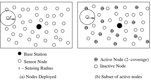
To improve energy efficiency of the network while maintaining fault tolerance from the subset of 2-coverage nodes previously chosen, the subset is further divided into 1-coverage nodes and backup nodes. Backup nodes provide additional support to the 1-coverage nodes in event detection and maintain fault tolerance. Backup nodes improve energy efficiency by reducing the communication as they only report when 1-coverage nodes fail to detect the event.

The selection process of subsetting of nodes is performed in different stages as part of the preprocessing of WSN to cater quality monitoring services.

• Selection of 2-coverage subset nodes

• Delaunay Triangulation over 2-coverage subset

• Selection of 1-coverage subset and backup nodes from selected 2-coverage subset.

(37)

0 1 0 1 0 1 0 1 01

0 1 0 1 ₀₁

0 1 0 1 0 1 0 1 0 1 0 1 0 0 1 1 Base Station Sensor Node r − Sensing Radius r

Inactive Node

Active Node (2−coverage)

(a) Nodes Deployed (b) Subset of active nodes

Figure 3.1: Subsetting of Nodes

subset provides 1-coverage and the other subset provides additional support or backup. Details of how the selection process is performed are presented in further sections below.

Considering a set ofSnodes in a given region, choosing the setDof minimum number of nodes, providing 2-coverage fromScan be represented as below:

D⊆S

Further dividing the set D into setsA andB, providing 1-coverage nodes and Backup nodes can be shown as below.

A⊆D

B⊆D

A∪B≡D

3.2.1 2 - Coverage

(38)

2-coverage for a given region is NP-hard, as mentioned before. To select the minimal number of nodes providing 2-coverage, we used the distributed greedy technique for K-coverage proposed in [53] and adapted it to provide 2-K-coverage. In the distributed greedy heuristic, a minimal number of nodes are selected from the deployed set. Initially, a random node, sayA, is chosen from the deployed setSand is identified as 2-coverage node.Anow broadcasts a control messageNODE-DBL-STATUS to its one-hop neighbors to select the potential 2-coverage node. The NODE-DBL-STATUS control message is used to query the one-hop neighbors if they are previously chosen as 2-coverage nodes. Upon receiving the NODE-DBL-STATUS message, the one-hop neighbors reply to the message received from Awith a control message YES/NO. The nodes notify A withYES if they have been previously chosen and NO if not chosen. Each and every node replies to the YES/NO control message three times to essentially make sure at least one of the control messages would make it to the node if other control message are dropped due to collisions.

(39)

connectivity between the sensor nodes in the network so that the nodes can transmit mes-sages and report events to the base station. Once the entire region is covered, the chosen 2-coverage sensor nodes are active and are involved in the sensing and communication activity of the network. The remaining nodes are inactive nodes.

Algorithm 1Distributed Greedy Algorithm

procedure2-COVERAGE(S[ ])

S[ ] is the set of sensor nodes deployed Ris the region to be covered

snode←S[x] .x is randomly selected node

while(Ris not Covered)do

dbl[i]←snode snode←broadcast() snode←recv()

snode←maxBeni f it() i←i+1

end while end procedure

3.2.2 Voronoi Diagrams and Delaunay Triangulation

Voronoi diagrams and Delaunay triangulations have found themselves a place in many domains of research. They have been very influential in solving the coverage problems of Wireless Sensor Networks. Voronoi diagrams are a set of discrete points in a 2D plane that partition the plane into a set of convex polygons such that all the points within a polygon are closest to only one site. One of the properties of Voronoi diagrams is that the adjacent polygons in a Voronoi diagram are equidistant from the edge dividing two neighboring sites in the construct. Figure 3.2(a) shows an example construct of a Voronoi diagram. Detailed explanation about Voronoi diagrams can be found in [3, 17]

(40)

(a) Voronoi diagram (b) Delaunay triangulation

Figure 3.2: Voronoi Diagram and Delaunay Triangulation of a Random Topology

(41)

performs triangulation, and checks for the validity of the Delaunay properties. Edges of the triangles are flipped to maintain the validity if the properties are not satisfied. Delaunay triangulation and its properties are presented in [17].

Once the 2-coverage set is chosen from the deployment, before performing Delaunay triangulation, every node broadcasts a control messageNODE-DBL-STATUSto identify the current active one-hop neighbors. Current active one-hop neighbors reply with aYES/NO control message to the broadcast message sent by the sender. After receiving theYES/NO message from the active one-hop neighbors in reply to NODE-DBL-STATUS message, every node performs a Delaunay triangulation over the one-hop neighboring nodes to choose backup nodes. Every node broadcasts aNODE-DBL-STATUSmessage the second time to maintain the current active nodes in the one-hop neighborhood and to perform a Delaunay triangulation over the current active node set. Using the one-hop neighbors containing the inactive nodes, which was previously gathered to find 2-coverage nodes, would increase the redundancy in the selection process. Every node broadcasting the NODE-DBL-STATUS message and replying with a YES/NO message is performed three times so that the control messages are not dropped due to collisions.

3.2.3 Selection of Backup Nodes

(42)

0 0 1 1

0

1

0 0 1 1 0 0 1 1

0

1

Backup A B C D E F G H I J K L M N P Q

J _E B

A C F K L M H G I N Q P D Primary (1−coverage)

(a) Double Set (2−coverage) (b) Backup Selection (Active Nodes)

Figure 3.3: Selection of Backup Nodes from Double Coverage Set

Algorithm 2Selection of Backup Nodes

procedureBKSELECT(dbl[ ])

dbl[ ] is the set of sensor nodes providing 2 - Coverage Neighbors[ ] is the set of Triangle Neighbors of each node i←0

whilei6=dbl.end()do

ifdbl[i].area()≡Neighbors[ ].area()then

backup[j]←dbl[i]

PotPri[]←nearest(Neighbors[],backup[j]) PotPri[]←median(Neighbors[],backup[j]) i←i+1

end if end while

whilei6=Pot_Pri.end()do

ifPotPri.area()≡Neighbors[ ].area()then

backup[]←PotPri[i] erase(PotPri[i])

(43)

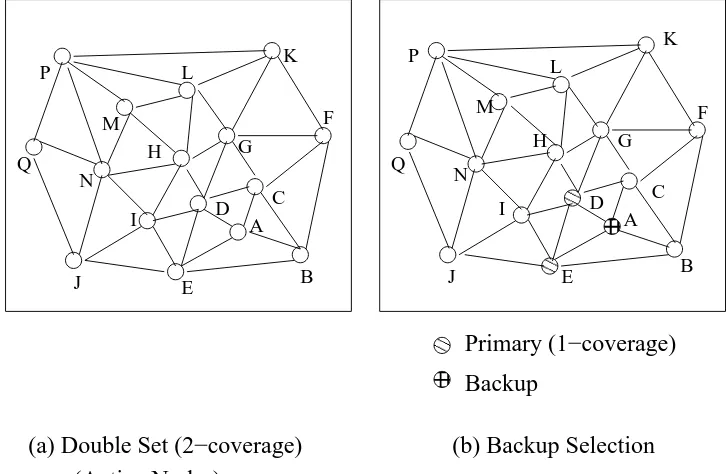
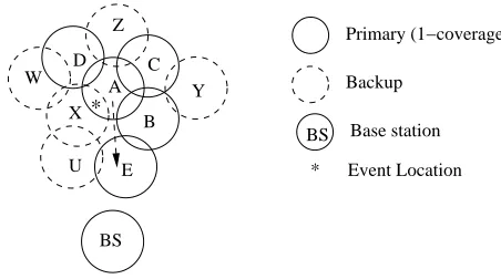
(1-coverage) nodes or not. Upon receiving reply control messages NODE-PRIMARY-STATUS-REPLY from one-hop neighbors B, C, D, E, and I, node A checks if the nodes that replied are present in the triangulation in which nodeAis a vertex. In this illustration, nodesB, C, D, andEare Delaunay neighbors in which nodeAis also part of the triangles. NodeAcomputes if it is a valid backup node by checking if the region it covers by itself is completely covered by the Delaunay neighbors. In the set of Delaunay neighbors, if nodeD is a backup node, then it is not considered in the computation. Only non-backup nodes are considered for computation. If the area is completely covered, then nodeAsets itself as a backup. Once a node is identified as a backup node, it sends a notification control message NODE-PRIMARY-STATUS-NOTIFY to the nearest and median distant neighbors, which areDandEin the illustration. To provide a better selection of 1-coverage nodes in the topology, nearest and median nodes are chosen. Nodes receiving the NODE-PRIMARY-STATUS-NOTIFY message will identify themselves as primary nodes providing 1-coverage. Nodes receiving theNODE-PRIMARY-STATUS-NOTIFY notification message would ignore the message if the node was previously identified as either a backup node or primary node. This process is performed in all nodes to identify backup and primary nodes. All the above processes are performed in stage one.

(44)

BS Base station Backup A

B C D

E

BS X

U

Y Z

W

*

* Event Location Primary (1−coverage)

Figure 3.4: Backup Functionality

nodes is also presented in the form of an algorithm.

3.3 Backup Node Functionality

For sensor nodes monitoring in harsh environments, several events go undetected due to noise interference, terrain, signal fading, obstacles, and etc. In order to provide additional support, backup nodes assist deployed 1-coverage nodes in detecting the event that occurred in a region. To illustrate the backup node functionality, we represent the network in Figure 3.4. Circles with solid boundaries are nodes providing 1-coverage, circles with dashed boundaries are backup nodes, and BS is base station.

3.3.1 Event Detection

(45)

base station. Backup nodes observe the packet transmissions for a time oft_d, which is the transmit time of a packet for one-hop to determine if the event was successfully detected by 1-coverage nodes. Backup nodes can overhear the packet transmissions, which is used to determine if the event was successfully detected. When 1-coverage nodes do not transmit packets for the event detection within the time t_d, the backup nodes classify the event detection as unsuccessful and transmit packets to its forwarder to report the event to the base station.

To illustrate the process of event detection in the WSN from Figure 3.4, consider that an event has occurred at location ‘*’. Node A and X have the event within their sensing region, and sense the event. NodeAtransmits packets to nodeEfor reporting the event to the base station. NodeEis the forwarder for nodeA, and forwards the packet received from Ato the base station. NodeX, as a backup node, will observe for a timet_d to overhear the packet transmission from node A. NodeX, upon overhearing the transmission from node A, considers the event to be successfully detected. If an unsuccessful detection occurs, X

would transmit the packet to its forwarder and report the event to base station.

3.3.2 Backup Reporting

(46)

which are 1-coverage nodes, overhear the transmission drop the packets at MAC layer as they are not destined to them. To perform the backup reporting functionality, packet transmissions overheard by the backup nodesU, X, Y, andZare not dropped at MAC layer, but forwarded to the Network layer of the backup node and cached. These cached packets are then transmitted in a different route when the backup node detects packet loss in the transmission. To detect packet loss during transmission between nodesA and E, backup nodes X and U within the one-hop neighborhood of Aand E only cache the packets and participate in further transmission. Nodes Y and Z do not cache the packets from nodeA as they cannot overhear the transmission from node E when further forwarded. Backup nodes determine the transmission of packets between nodeAandEas successful if backup nodes overhear the transmission of the same packet from nodeE to its forwarder, which was previously sent from nodeA. In this process, backup nodes have to wait for a threshold time, and would transmit if there is an unsuccessful transmission between nodesAandE. As an optimization, backup nodes do not cache the packets whose next hop is the base station.

(47)

3.4 Event Reporting

In a WSN, events occur at random locations and these events not only must be detected, but also successfully reported to the base station. The primary traffic pattern in WSN is

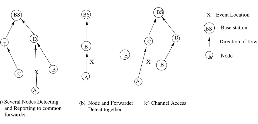
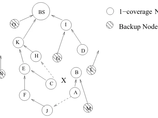
convergecast(sensor-to-sink) in reporting events, that is sensor nodes sending messages to the base station. In a WSN, sensors choose their forwarders based on the distance from the node to the base station. The one-hop neighbor nearest to the base station is chosen as the forwarder. When there are two or more nodes detecting an event at the same time, there arises a complicated case of convergecast traffic pattern, also known asspatially-correlated contention. When several nodes detect the same event and report the event to its forwarder,

several packets are dropped due to collisions in the network, thereby reducing the number of events reported to the base station. Predominant problem scenarios in random deployment leading to contention and congestion are as follows:

• Several nodes detecting and reporting events to a common forwarder.

• A node and its forwarder detecting the event.

• Channel access issues.

(48)

(a) Several Nodes Detecting _(b) _(c) A B C D E A B A E C B D

BS BS BS

X X

BS Base station X Event Location

Direction of flow

X

Node A

and Reporting to common forwarder

Node and Forwarder Detect together

Channel Access

Figure 3.5: Event Reporting

the forwarder for nodeAand node Dis the forwarder for nodeB. NodeAandBtransmit packets simultaneously, and node C, being within the one-hop neighborhood of node B, overhears the transmissions of nodeBand packets from nodeAare dropped due to channel access.

(49)

000 000 000 111 111 111 000 000 000 111 111 111 00 00 00 11 11 11 00 00 11 11 00 00 11 11 00 00 11 11 0000 1111 BS O K H E F J C A B I D N G L M X Backup Node 1−coverage Node

Figure 3.6: Spatially correlated contention

timer implemented. Nodes choose the node providing 1-coverage as the forwarder, which is not within the one-hop neighborhood of other sensing nodes detecting the event. If the 1-coverage node sensing the event cannot find an alternate route with primary nodes in the one-hop neighborhood, it would forward the packet to the backup node to report the event to base station. In this way, event reporting is performed better by handling collisions and contention in the network.

(50)

CHAPTER 4 PERFORMANCE EVALUATION

To evaluate the performance, the proposed protocol is implemented in the ns-2 simulator [1]. Extensive experiments were conducted in order to test the performance of the pro-posed coverage protocol. First, the propro-posed approach is compared with 1-coverage and 2-coverage in terms of standard metrics, such as active node count ratio, coverage ratio, and energy consumption. Second, the proposed approach is evaluated for fault tolerance and event reporting in terms of event detections and event reporting as specific metrics and compared with 1-coverage and 2-coverage.

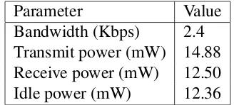
The simulations were run with the simulation parameters from the literature [51], as mentioned in Table 4.1 and Table 4.2, in an area of 100m x 100m, transmission radius of 15m, and a sensing radius of 7.5m. All the sensors are randomly deployed and the simulation results are averaged for 20 randomly distributed topologies. In all the experi-ments, to evaluate the standard metrics presented, each data point taken is an average of 20 independent runs with random seeds for each topology.

4.1 Fault Tolerance

(51)

Parameter Value Bandwidth (Kbps) 2.4 Transmit power (mW) 14.88 Receive power (mW) 12.50 Idle power (mW) 12.36 Table 4.1: Parameters for Low Power

Parameter Value

Bandwidth (Kbps) 100 Transmit power (mW) 660 Receive power (mW) 395 Idle power (mW) 350 Table 4.2: Parameters for High Power

0 50 100 150 200 250

0 200 400 600 800 1000

Active Nodes

Total Nodes Deployed 1-coverage Nodes

Backup Nodes 2-coverage Nodes

(52)

of the WSN, coverage ratio, active node count ratio, and event detection ratio are used as metrics. To measure the performance in terms of active nodes count and coverage ratio, simulations are run by varying the number of sensors randomly distributed in the region from 100 to 1000 nodes on a 100m x 100m region to evaluate the performance of active node count ratio and coverage ratio.

Figure 4.1 shows that, the subset of active nodes chosen to provide 2-coverage, 1-coverage and backup is consistently maintained from nodes greater than 400. This behav-ior is observed with nodes greater than 400 for the given geographical region, since the selection of minimal number of 2-coverage nodes from the distribution is not influenced by the location of the nodes as the network is over-provisioned. As the 1-coverage and backup nodes are chosen as subsets from 2-coverage set, similar behavior for both the subsets is expected. The difference between the number of active nodes in 1-coverage, backup, and 2-coverage for network size below 300 nodes is due to an insufficient number of nodes to choose to cover the entire region. The gap between the number of nodes providing 1-coverage and backup nodes for deployment of nodes greater than 400 is due to: (a) the influence of the random nature in the selection of 2-coverage nodes, (b) the selection of 1-coverage nodes as backup nodes and vice versa, (c) the division of 2-coverage nodes into exact halves is not possible as there could be an odd number of nodes chosen.

(53)

0 20 40 60 80 100

0 200 400 600 800 1000

Coverage Ratio

Total Nodes Deployed 1-coverage Nodes

Backup Nodes 2-coverage Nodes

Figure 4.2: Coverage Ratio vs Number of Nodes Deployed

the nodes chosen as 1-coverage can be chosen as backup and vice versa).

(54)

0 20 40 60 80 100

0 1 2 3 4 5

Percentage of Events Detected

Percentage of Nodes Failed (200 Nodes) 1-coverage Backup Coverage

(a) 1-Coverage vs Backup (200 Nodes)

0 20 40 60 80 100

0 1 2 3 4 5

(b) Backup vs 2-coverage (200 Nodes)

0 20 40 60 80 100

0 1 2 3 4 5

(c) 1-Coverage vs Backup (500 Nodes)

0 20 40 60 80 100

0 1 2 3 4 5

(d) Backup vs 2-coverage (500 Nodes)

0 20 40 60 80 100

0 1 2 3 4 5

(e) 1-Coverage vs Backup (800 Nodes)

0 20 40 60 80 100

0 1 2 3 4 5

(f) Backup vs 2-coverage (800 Nodes)

(55)

a subset of nodes providing 1-coverage in the backup coverage set are only considered for failures to match the number of nodes for a 1-coverage protocol. The percentage of event detections for backup coverage and 2-coverage is equal, as the same set of nodes is considered for node failures.

4.2 Event Reporting

For sensor networks to provide quality service, sensors not only have to detect the events but also report them. Simulations were run by generating 100 events at random times to observe event reporting in the WSN. Sensors placed at random positions to monitor a given region in harsh environments have sporadic events occurring at different locations. To distinguish between events, each event is uniquely identified by sensor nodes based on the location and the timestamp. Two nodes can distinguish between events occurring at the same location at different times or within the common sensing region of the nodes at the same time based on the unique event identification numbers, which the nodes generate at the time of event detection. For sensors to send data packets for the events generated, constant bit rate (CBR) traffic of packet size 64 bytes is generated for high, medium, and low traffic loads. Each event is simulated for a period of 10 seconds, which is sufficient enough for an event to be reported. The threshold value for the number of packets required to reach the base station for an event to be reported is application specific. Simulations were run in non congested scenario and the total number of packets received at the base station for all events with 2-coverage was observed as 75%. Based on the observation of the number of packets received at the base station, we chose the threshold value for required number of packets as 75% to report an event.

(56)

0 20 40 60 80 100

0 1 2 3 4 5

Percentage of Events Reported

Percentage of Nodes Failed 1-coverage Backup Coverage

(a) 1-Coverage vs Backup (Low Power)

0 20 40 60 80 100

0 1 2 3 4 5

(b) Backup vs 2-coverage (Low Power)

0 20 40 60 80 100

0 1 2 3 4 5

(c) 1-Coverage vs Backup (High Power)

0 20 40 60 80 100

0 1 2 3 4 5

(d) Backup vs 2-coverage (High Power)

(57)

0 20 40 60 80 100

0 1 2 3 4 5

0 20 40 60 80 100

0 1 2 3 4 5

0 20 40 60 80 100

0 1 2 3 4 5

0 20 40 60 80 100

0 1 2 3 4 5

(58)

0 20 40 60 80 100

0 1 2 3 4 5

0 20 40 60 80 100

0 1 2 3 4 5

0 20 40 60 80 100

0 1 2 3 4 5

0 20 40 60 80 100

0 1 2 3 4 5

(59)

used to study the behavior of event reporting for different network loads. With parameters in low power/high power settings, backup coverage has outperformed both 1-coverage and 2-coverage in terms of event reporting in high, medium, and low network loads of 0.2, 0.4 and 0.6 packets/sec. With low power settings and a high network load of 0.2 packets/sec, the performance by 2-coverage in event reporting is very low. This is due to reasons of congestion and spatially-correlated contention in the network. Performance of event reporting by 1-coverage nodes with low power settings was better than 2-coverage. The initial expectation was a fault tolerant network, such as 2-coverage, to perform better over 1-coverage in event reporting. However, issues related to spatially-correlated contention, as explained in Chapter 3 and congestion in the network have reduced the performance of event reporting by 2-coverage nodes. The 1-coverage performs better as a number of sensors detecting the events is less, thereby reducing the communication traffic in the network. The enhanced performance of backup coverage over 2-coverage and 1-coverage is due to the cross-layered network protocol design, which helps backup nodes to improve the reporting of events to the base station when there are packet losses in the network. Also, reduced communication in the network helps in enhancing the event reporting, since backup nodes come into service only when 1-coverage nodes fail to detect the event. Per-formance of all the techniques for medium and low network loads is better in comparison with a high network load due to less congestion, as can be observed from Figures 4.4, 4.5, and 4.6.

(60)

0 200 400 600 800 1000 1200

0 200 400 600 800 1000

Energy(J)

Number of Nodes

1-Coverage Backup Coverage 2-Coverage

(a) Energy(Low Power) v/s Number of Nodes

0 2000 4000 6000 8000 10000 12000 14000

0 200 400 600 800 1000

Energy(J)

Number of Nodes

(b) Energy(High Power) v/s Number of Nodes

Figure 4.7: Energy Consumed (High Load) vs Number of Nodes

0 200 400 600 800 1000 1200

0 200 400 600 800 1000

Energy(J)

Number of Nodes

0 2000 4000 6000 8000 10000 12000 14000

0 200 400 600 800 1000

Energy(J)

Number of Nodes

Figure 4.8: Energy Consumed (Medium Load) vs Number of Nodes

the energy consumed is very high.

4.3 Energy Efficiency

(61)

0 200 400 600 800 1000 1200

0 200 400 600 800 1000

Energy(J)

Number of Nodes

0 2000 4000 6000 8000 10000 12000 14000

0 200 400 600 800 1000

Energy(J)

Number of Nodes

Figure 4.9: Energy Consumed (Low Load) vs Number of Nodes

observed for a packet size of 64 bytes at high, medium, and low network loads of 0.2, 0.4, and 0.6 packets/sec, respectively. From Figures 4.7, 4.8, and 4.9, there is more energy consumption for high parameter settings over the low parameter settings. For different network loads, the energy consumed varied for both low and high parameter settings. The energy consumption is more at a high network load of 0.2 packet/sec in both low and high parameter settings in comparison with medium and low network loads 0.4 and 0.6 packets/sec as more number of packets are transmitted. This increase in energy consumption is due to an increased number of transmissions as the network loads increase.

(62)

the energy consumed is increased.

In high power settings, the difference between 2-coverage and backup coverage is much larger when compared to low power settings. Also, with high power settings, there is an improved event reporting for all 1-coverage, backup, and 2-coverage techniques and less congestion in the network. With low congestion in the network, there is more energy consumption for 2-coverage, and less consumption for backup coverage. Similar behavior differences in energy consumption between 2-coverage and backup coverage for an increase in network load is shown in Figures 4.7, 4.8, and 4.9, with respect to low power settings.

(63)

CHAPTER 5 CONCLUSIONS

Wireless Sensor Networks are mainly deployed in harsh environments to provide quality services. In such environments, errors in WSN like noise interference, terrain, and obstacles pose problems in detecting the event and thereby degrade the event detection capability of the network. There is a need to provide fault tolerance to detect the events occurring in the geographical region. With current fault tolerant mechanisms, many nodes detect the same event and forward data to the base station, which increases the number of transmissions and congestion in the network. With an increase in the number of transmissions, the energy consumption of nodes increases and the event reporting capability due to collisions in the network is reduced. A decrease in the number of events reported to the base station reduces the quality of service provided by the coverage protocol. Also, as sensor nodes are energy constrained, maintaining energy efficiency is one of the primary concerns of sensor networks. To provide quality service by coverage protocols, there arises a need for developing protocols to provide fault tolerance, event reporting, and maintain energy efficiency.

(64)

trans-port layer and MAC, our coverage protocol provides fault tolerance, and event retrans-porting while reducing energy consumption.

Our simulation results show that the proposed coverage protocol provides fault tol-erance, and improve event reporting. Backup coverage, in comparison with 1-coverage, consumes more energy, but the quality of service provided is better. The number of events detected by backup coverage is the same as 2-coverage, the energy consumed is high and the event reporting has significantly suffered in 2-coverage, while backup coverage has less energy consumption and superior event reporting.

(65)

REFERENCES

[1] The Network Simulator: NS-2. http://www.isi.edu/nsnam/ns.

[2] O. B. Akan and I. F. Akyildiz. ESRT: Event-to-Sink Reliable Transport in Wireless Sensor Networks. Networking, IEEE/ACM Transactions on, 13(5):1003–1016, Octo-ber 2005.

[3] F. Aurenhammer. Voronoi diagrams—A Survey of a Fundamental Geometric Data Structure. ACM Comput. Surv., 23(3):345–405, 1991.

[4] M. Cardei, M. T. Thai, Y. Li, and W. Wu. Energy-Efficient Target Coverage in Wireless Sensor Networks. In INFOCOM, 24th Annual Joint Conference of the IEEE Computer and Communications Societies. Proceedings IEEE, volume 3, pages 1976–1984, March 2005.

[5] M. Cardei, J. Wu, M. Lu, and M. O. Pervaiz. Maximum Network Lifetime in Wireless Sensor Networks with Adjustable Sensing Ranges. InWireless And Mobile Computing, Networking And Communications, IEEE International Conference on, volume 3, pages 438–445, August 2005.

[6] A. Cerpa and D. Estrin. ASCENT: Adaptive Self-Configuring sEnsor Networks Topologies. Mobile Computing, IEEE Transactions on, 3(3):272–285, July 2004.

[7] K. Chakrabarty, S. Iyengar, H. Qi, and E. Cho. Grid Coverage for Surveillance and Target Location in Distributed Sensor Networks.IEEE Trans. Comput., 51(12):1448– 1453, 2002.

[8] B. Chen, K. Jamieson, H. Balakrishnan, and R. Morris. Span: An Energy-Efficient Coordination Algorithm for Topology Maintenance in Ad Hoc Wireless Networks. Wirel. Netw., 8(5):481–494, 2002.

[9] Bogdan C˘arbunar, Ananth Grama, Jan Vitek, and Octavian C˘arbunar. Redundancy and coverage detection in sensor networks. ACM Trans. Sen. Netw., 2(1):94–128, 2006.

(66)

Intelligence, Networking, and Parallel/Distributed Computing, SNPD, Seventh ACIS International Conference on, pages 285–289, June 2006.

[11] H. Gupta, Z. Zhou, S. R. Das, and Q. Gu. Connected Sensor Cover: Self-Organization of Sensor Networks for Efficient Query Execution. IEEE/ACM Trans. Netw., 14(1):55–67, 2006.

[12] M. Hefeeda and M. Bagheri. Randomized k-Coverage Algorithms For Dense Sensor Networks. InINFOCOM, 26th IEEE International Conference on Computer Com-munications. IEEE, pages 2376–2380, May 2007.

[13] C. Hsin and M. Liu. Network Coverage Using Low Duty-Cycled Sensors: Random and Coordinated Sleep Algorithms. InInformation Processing in Sensor Networks, IPSN, Third International Symposium on, pages 433–442, April 2004.

[14] C. Hsin and M. Liu. Randomly Duty-cycled Wireless Sensor Networks: Dynamics of Coverage. Wireless Communications, IEEE Transactions on, 5(11):3182–3192, November 2006.

[15] C. Huang and Y. Tseng. The Coverage Problem in a Wireless Sensor Network. In WSNA: Proceedings of the 2nd ACM international conference on Wireless sensor networks and applications, pages 115–121, New York, NY, USA, 2003. ACM.

[16] K. Jamieson, H. Balakrishnan, and Y. C. Tay. Sift: A MAC Protocol for Event-Driven Wireless Sensor Networks, volume 3868. Springer Berlin / Heidelberg, 2006.

[17] J. G. Leonidas, D. E. Knuth, and M. Sharir. Randomized Incremental Construction of Delaunay and Voronoi Diagrams, volume 7. Springer New York, 1992.

[18] X. Li, G. Calinescu, P. Wan, and Y. Wang. Localized Delaunay Triangulation with Application in Ad Hoc Wireless Networks. Parallel and Distributed Systems, IEEE Transactions on, 14(10):1035 – 1047, October 2003.

[19] X. Li, P. Wan, and O. Frieder. Coverage in Wireless Ad Hoc Sensor Networks. Computers, IEEE Transactions on, 52(6):753–763, June 2003.

[20] Md. Mamun-Or-Rashid, Md. Mahbub, Md. A. Razzaque, and C. S. Hong. Reliable Event Detection and Congestion Avoidance in Wireless Sensor Networks, volume 4782. Springer Berlin / Heidelberg, 2007.