www.geosci-model-dev.net/2/1/2009/
© Author(s) 2009. This work is distributed under the Creative Commons Attribution 3.0 License.
Geoscientific
Model Development
qtcm
0.1.2: a Python implementation of the Neelin-Zeng
Quasi-Equilibrium Tropical Circulation Model
J. W.-B. Lin
Physics Department, North Park University, 3225 W. Foster Ave., Chicago, Illinois 60625, USA Received: 23 September 2008 – Published in Geosci. Model Dev. Discuss.: 30 October 2008 Revised: 2 February 2009 – Accepted: 2 February 2009 – Published: 11 February 2009
Abstract. Historically, climate models have been devel-oped incrementally and in compiled languages like Fortran. While the use of legacy compiled languages results in fast, time-tested code, the resulting model is limited in its mod-ularity and cannot take advantage of functionality avail-able with modern computer languages. Here we describe an effort at using the open-source, object-oriented language Python to create more flexible climate models: the package qtcm, a Python implementation of the intermediate-level Neelin-Zeng Quasi-Equilibrium Tropical Circulation model (QTCM1) of the atmosphere. The qtcm package retains the core numerics of QTCM1, written in Fortran to optimize model performance, but uses Python structures and utilities to wrap the QTCM1 Fortran routines and manage model ex-ecution. The resulting “mixed language” modeling package allows order and choice of subroutine execution to be altered at run time, and model analysis and visualization to be in-tegrated in interactively with model execution at run time. This flexibility facilitates more complex scientific analysis using less complex code than would be possible using tradi-tional languages alone, and provides tools to transform the traditional “formulate hypothesis→write and test code→
run model→analyze results” sequence into a feedback loop that can be executed automatically by the computer.
1 Introduction
Although early weather and climate models, beginning with Richardson’s “Forecast Factory” in 1922 (Edwards, 2000), led the development of the field of scientific computing, over the past few decades, climate models have not, in general, kept up with advances in computing languages and
struc-Correspondence to: J. W.-B. Lin ([email protected])
tures. Many climate models are still written in compiled languages (primarily Fortran), and utilize the same program-ming structures familiar to a Fortran programmer of the 1970’s. On the positive side, this continued reliance on For-tran results in very fast code that runs on almost all platforms, the ability to reuse legacy code, and the availability of well-tested libraries, which have been optimized over decades of use.
At the same time, the continued development of climate models in Fortran has made it difficult to utilize program-ming language advances that increase the modularity and ro-bustness of scientific code. Being mainly a procedural lan-guage, Fortran has traditionally lacked the default program-ming structures to organize a model into truly self-contained units, thus limiting modularity. Fortran subroutine function calls may utilize long and unwieldy argument lists, its de-fault variables are not self-describing, and variables exist in a loosely controlled namespace; this can result in brittle code where undetectable errors easily propagate. Finally, as a compiled language, Fortran is non-interactive and requires separate compiling and linking steps. This hinders informal small-scale testing, prevents users from interacting with the model at run time, and can result in a longer development cycle. Recent versions of Fortran (e.g., Fortran 95, 2003) have added some of these modern features to the language, but scientific programs, in general, make limited use of these new features.
variables make possible additional levels of modular de-composition. Object-oriented programming can also pro-duce code of higher quality (e.g., Johnson, 2002), that more closely emulates real-world entities (e.g., Pennington et al., 1995). Some modern languages are also interpreted; in those languages, source code is directly executed at run time with-out separate compiling and linking steps, thereby enabling interactive debugging and execution.
One such modern language is Python (van Rossum, 2008), an interpreted, object-oriented, multi-platform, open-source language used in a variety of software applications, including as a robust scientific computing platform (Oliphant, 2007). In climate studies, Python has been used as the core lan-guage for data analysis (e.g., PCMDI, 2006), visualization (e.g., Hunter and Dale, 2007), and modeling (e.g., PyCCSM, 2008). Python’s object-orientation and higher-level data structures and tools (e.g., dictionaries, string and file utilities) permits numerous ways of decomposing a model into mod-ular units. Its extensive suite of higher-level analysis tools (e.g., statistics, visualization), accessible at run time, enables modeling and analysis to occur concurrently. As an inter-preted language, Python’s lack of a separate lengthy compile step greatly simplifies debugging and testing, and permits changes in the program to be made at run time.
While it is more difficult to write robust code in compiled languages, the code is usually very fast. Modern languages, however, while producing much more robust and stable code, exact a cost in performance. Naturally, we want the best of both worlds, both speed and simplicity: “mixed language” environments (Oliphant, 2007) are a solution. In such an en-vironment, the user-interface and calling infrastructure of the model is written in a modern language while the performance sensitive code is written in a compiled language. A wrap-per generator automatically creates extension modules (as shared object libraries) of the compiled language modules, making them accessible to the modern language. A number of wrapper generator packages exist for Python, including f2py(Peterson, 2005) which wraps Fortran modules, and SWIG (Beazley, 1997) which wraps C/C++ code.
In the present work, we describe a Python implementa-tion of an intermediate-level atmospheric circulaimplementa-tion model originally written in Fortran. By wrapping the Fortran code within a Python object structure, the package, qtcm, pro-vides a modular and interactive model where the user can alter order and choice of subroutine execution, and analyze and visualize model results, all dynamically at run time. The result is a climate modeling environment that can transform parts of the “formulate hypothesis→write and test code→
run model→analyze results” sequence into a feedback loop that can be executed automatically by the computer.
Section 2 briefly describes the Neelin-Zeng Quasi-Equilibrium Tropical Circulation Model (QTCM1). In Sect. 3, we describe the construction of a Python implemen-tation of QTCM1, theqtcmpackage. Section 4 gives ex-amples of the use of theqtcmpackage, which illustrate the
benefits of a mixed language environment for climate mod-eling. We finish with discussion and conclusions in Sect. 5.
2 The Neelin-Zeng QTCM1
The QTCM1 is a primitive equation-based intermediate-level atmospheric model that focuses on simulating the tropical atmosphere (Neelin et al., 2002). Being more complicated than a simple model, the model retains full non-linearity with a basic representation of baroclinic instability, includes a radiative-convective feedback package, and includes a sim-ple land soil moisture routine (but does not include topog-raphy). The QTCM1 has been used in a variety of studies, including investigations of Madden-Julian oscillation main-tenance mechanisms (Lin et al., 2000), stochastic convec-tive parameterization (Lin and Neelin, 2000, 2002), El Ni˜no-Southern Oscillation teleconnection patterns (Gushchina et al., 2006), and vegetation-atmosphere interactions (Zeng et al., 1999).
QTCM1 differs from most full-scale general circulation models (GCMs) in that the vertical temperature, humidity, and velocity structures of the atmosphere are represented by a truncated Galerkin expansion in the vertical, instead of finite-differenced pressure levels. The vertical basis func-tions of the expansion are chosen based on analytical so-lutions under convective quasi-equilibrium conditions, and thus in the tropics, where convective quasi-equilibrium ef-fects dominate, the solution is asymptotically exact. Away from the tropics, the model behaves as a two-layer model. In principle, a Galerkin model can have any number of baroclinic basis functions accompanying its barotropic basis: QTCM1 has a single baroclinic mode, and hence the “1” in its name. In the horizontal, the model discretizes the domain using a staggered Arakawa C-grid (Mesinger and Arakawa, 1976) and a default resolution of 5.625◦longitude by 3.75◦ latitude.
By using tailored vertical profiles, the QTCM1 delivers reasonable simulations of the tropics at a fraction of the com-putational cost of a full-scale GCM. Its relative simplicity also makes it far easier to diagnose than a full-scale GCM, potentially resulting in greater understanding and compre-hension of model results. Neelin and Zeng (2000) presents a comprehensive description of the model’s formulation, and Zeng et al. (2000) describes the model’s climatology. A de-tailed manual (Neelin et al., 2002) describes the structure of the Fortran code. Neelin and Zeng (2000) is based upon v2.0 of QTCM1 and Zeng et al. (2000) is based on QTCM1 v2.1. Theqtcmpackage is based on QTCM1 v2.3.
3 The Pythonqtcmpackage
modules (as shared object libraries). At the package home page (http://www.johnny-lin.com/py pkgs/qtcm/), the full source code and a comprehensive user’s guide is available for download. The User’s Guide and source code for the ver-sion of the model described in the present work is available as a supplement at http://www.geosci-model-dev.net/2/1/2009/ gmd-2-1-2009-supplement.zip, and are covered by licenses separate from the present work. The User’s Guide (Lin, 2008) provides detailed information regarding installing, us-ing, troubleshootus-ing, and adding code to the package. In the present work, we provide an overview ofqtcm’s structure and function. Parts of this section are copied and/or adapted from Lin (2008).
3.1 Object-oriented programming
Because Python is an object-oriented language, the funda-mental programming unit is not the subroutine, but instead is the “object”. In a procedural language, data and functions that operate on data are two separate entities. In an object-oriented language, these two entities are bound together in a single construct, the object. Because of this framework, functions are automatically considered in context with the data they operate on, and vice versa. This lessens the risk of errors that occur when data is manipulated by functions that were never intended to be used on that kind of data.
Data bound to an object are called “attributes” of that object, and functions that operate on that data are called “methods” of that object. In Python, the attributes of an object are specified by a name that comes after a period at the end of the object name. Thus, model.runname refers to the runname attribute of the model ob-ject. Methods are similarly named; however, to call a method, a parameter list (even if empty) must be specified. Thus,model.run session()calls therun session method bound to themodelobject.
In general, Python objects consist of two types of attributes and methods: public and private. Public attributes and meth-ods are accessible to the general user. Private attributes and methods, on the other hand, are designed to be accessed only by developers. In Python, private attributes and methods have names prepended by one or two underscores.
Objects are created from a “template” that defines the at-tributes and methods that go into that object. The template is known as a “class,” and individual objects that are derived from a class are called “instances” of that class. Creating an object that is an instance of a class is known as “instantiat-ing” the object. In the example above,modelis an instance of theQtcmclass, which defines therunnameattribute and run sessionmethod. There is no limit to the number of instances of a class, and all instances of a class have access to the attributes and methods defined by the class.
Python’s highest level of organization is the package, a li-brary of related modules. Modules, in Python, are individual files that define related objects, functions, and variables, and
thus a package is a directory of module files. A single mod-ule can contain an unlimited number of objects, functions, and variables.
3.2 Package and model structure
The qtcm package consists of two shared object libraries and four main submodules. The two shared object libraries are compiled and generated byf2pyduring package instal-lation, and will not need to be recompiled prior to model exe-cution. Thedefaultssubmodule defines various defaults for the model, thefieldsubmodule defines classField (key model variables and parameters are instances of this class), theplotsubmodule defines routines used for quick visualization of model results, and theqtcmsubmodule de-fines the classQtcm(which defines model objects).
A model in the qtcmpackage is defined as an instance of the classQtcm. Because theqtcmpackage wraps For-tran routines with a Python layer, there are two types of variables associated withQtcmmodel instances: those de-fined at the Python-level and those dede-fined at the Fortran-level. Some variables, while defined separately at both the Python and Fortran levels (i.e., they do not share the same memory space), have the same names and functions in both levels of the model. Those variables are known as “field vari-ables” and are considered to be defined at both the Python-level and Fortran-Python-level (an example of such a variable is Qc, the precipitation). Qtcm instances have public meth-ods (get qtcm1 itemandset qtcm1 item) for pass-ing the values of field variables back-and-forth between the Python and Fortran levels.
All field variables and most model parameters (such as time step, input and output directory names, etc.) are in-stances of theFieldclass. AField instance stores the value of the variable in an attribute namedvalue, and meta-data (e.g., units, long name, etc.) related to the variable as other instance attributes. If the value of the field variable is an array, the value stored in the attributevalueis a NumPy (van der Walt, 2008) array. Only the value of aField in-stance can be passed to its Fortran counterpart (when it ex-ists), because standard Fortran variables cannot hold meta-data.
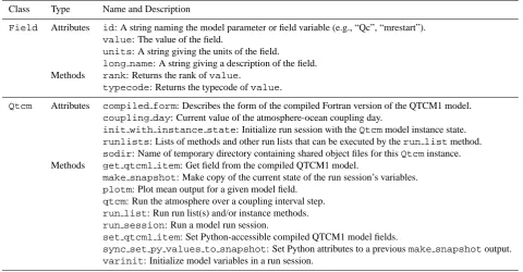
Table 1. Key public instance attributes and methods forFieldandQtcminstances. Note that forQtcminstances, field variables are also attributes, with attribute names corresponding to the ids of the fields.
Class Type Name and Description
Field Attributes id: A string naming the model parameter or field variable (e.g., “Qc”, “mrestart”). value: The value of the field.
units: A string giving the units of the field.
long name: A string giving a description of the field. Methods rank: Returns the rank ofvalue.
typecode: Returns the typecode ofvalue.
Qtcm Attributes compiled form: Describes the form of the compiled Fortran version of the QTCM1 model. coupling day: Current value of the atmosphere-ocean coupling day.
init with instance state: Initialize run session with theQtcmmodel instance state. runlists: Lists of methods and other run lists that can be executed by therun listmethod. sodir: Name of temporary directory containing shared object files for thisQtcminstance. Methods get qtcm1 item: Get field from the compiled QTCM1 model.
make snapshot: Make copy of the current state of the run session’s variables. plotm: Plot mean output for a given model field.
qtcm: Run the atmosphere over a coupling interval step. run list: Run run list(s) and/or instance methods. run session: Run a model run session.
set qtcm1 item: Set Python-accessible compiled QTCM1 model fields.
sync set py values to snapshot: Set Python attributes to a previousmake snapshotoutput. varinit: Initialize model variables in a run session.
from qtcm import Qtcm inputs = {}
inputs[’runname’] = ’test’ inputs[’landon’] = 0 inputs[’year0’] = 1 inputs[’month0’] = 11 inputs[’day0’] = 1 inputs[’lastday’] = 30 inputs[’mrestart’] = 0
inputs[’compiled form’] = ’parts’ model = Qtcm(**inputs)
model.run session()
Fig. 1. A simpleqtcmrun.
3.3 Creating a model instance and running the model Figure 1 shows a simple example of a model instance being created and run. Model instances are created using standard Python syntax; in Fig. 1, model = Qtcm(**inputs) creates a model instancemodel. In this example, we make use of a feature in Python where keyword parameter argu-ment lists can be passed in as a dictionary (a set of key/value pairs), where the dictionary’s keys correspond to the names of the keyword parameters, and the associated value in the dictionary corresponds to the input value of the keyword pa-rameter; the variableinputsis such a dictionary. Based on the values ofinputsshown in Fig. 1, the model instance
is configured to make an aquaplanet run (set bylandon), starting from November 1, Year 1 (set byyear0,month0, and day0), running for 30 days (set by lastday) from a newly initialized model state (set by mrestart). The model’s netCDF (Unidata, 2007) output filenames will con-tain the string given by runname. By default, the model uses climatological sea-surface temperatures (SST) for the lower-boundary forcing over the ocean.
The keywordcompiled formdefines which of the two types of Fortran extension modules, derived from the For-tran QTCM1 code, the model instance will link to. The first type permits very little control over the compiled For-tran routines at the Python level, and is selected by set-ting compiled form = ’full’. The second allows a user, from the Python-level, to control model execution in the Fortran-level all the way down to the atmospheric timestep level. This extension module is selected by setting compiled form = ’parts’. In general, most users will setcompiled form = ’parts’, and thus we assume this setting for the rest of the present work. See Lin (2008) for details about this keyword.
3.4 Run sessions
Once we instantiate and configure a model instance, we can use the instance for any number of runs. We call each of these runs using the same model instance a “run session.” In a run session, the model is run from day 1 of simulation to the day specified by thelastdayattribute. A run session is a “complete” model run, at the beginning of which all Fortran-level field variables are set to the values given at the Python-level, and at the end of which restart files are written, the values at the Python-level are overwritten by the values from the Fortran-level, and a Python-accessible snapshot is taken of the model variables that were written to the restart file.
Before and after a run session, model variables are easily accessed from the Python level, and can be changed at will just by changing the value of the pertinent model instance attribute. The new values can then be used at the next run session of the model instance. To continue a second run ses-sion after an initial run sesses-sion, set the keyword parameter contin the input list of arun sessionmethod call.
Figure 2 gives an example of two run sessions, where the second run session is a continuation of the first, and with changes made to a field variable between the two run ses-sions. The first run session lasts 10 days, and is given by the setting of thelastdaykeyword parameter. Between these run sessions, the value of field variableu1(the zonal wind associated with the first baroclinic mode) is doubled, and this doubled value is used in the second run session. The second run session lasts 30 days.
The change between the two run sessions in the simple ex-ample given in Fig. 2 is uninteresting, but the exex-ample illus-trates how theqtcmPython framework opens up possibili-ties of interactive analysis with the model. Because Python is an interpreted language, the code in Fig. 2 does not have to be written in a file, compiled, linked, and executed; the code can be typed in during run time. Between run ses-sions, we can conduct and visualize more complex analyses of the model, and use the results of those analyses to change the model configuration for the next run session. And since Python is a complete programming language, we can also automate these analyses, without leaving the modeling envi-ronment. The important benefits of this feature are described in Sect. 4.
3.5 Passing restart snapshots between run sessions Sometimes, we want to branch a number of model runs from the same starting point. The QTCM1 writes restart files for that purpose, and aQtcminstance can also make use of those files by setting themrestart attribute accordingly. This restart mechanism is straightforward to use, but becomes dif-ficult to manage when many restart files are involved.
Theqtcmpackage provides a way to take, store, and ap-ply restart snapshots at the Python-level, by storing a shot as a dictionary. At the end of a run session, a
snap-inputs[’year0’] = 1 inputs[’month0’] = 11 inputs[’day0’] = 1 inputs[’lastday’] = 10 inputs[’mrestart’] = 0
inputs[’compiled form’] = ’parts’
model = Qtcm(**inputs) model.run session()
model.u1.value = model.u1.value * 2.0 model.init with instance state = True model.run session(cont=30)
Fig. 2. An example of twoqtcmrun sessions where the second run session is a continuation of the first. Assumeinputs is a dictionary as in Fig. 1, and that earlier in the script the run name and all input and output directory names were added to the dictionary.
shot of the model state is automatically taken and stored as the instance attribute snapshot. The snapshot in-cludes the date of the model and prognostic variables like T1. You can store this attribute as another Python vari-able for later use. Figure 3 shows an example of sav-ing the model snapshot as the variablemysnapshot, and using that snapshot to initialize a later run session. The methodsync set py values to snapshotinitializes the model to the values ofmysnapshot, and setting the attributeinit with instance statetoTrueprior to callingrun sessionthe second time will force the model to use the current instance state as the run session’s initial values.
3.6 Creating multiple models
Creating multiple QTCM1 Fortran models requires maintain-ing and operatmaintain-ing on different sets of source code, as well as compiling each set of source code separately to obtain the de-sired multiple executables. With theqtcmpackage, creating multiple models is as easy as instantiating multipleQtcm in-stances. For instance, to create two Python QTCM1 models, model1andmodel2, just enter in the following:
from qtcm import Qtcm model1 = Qtcm(**inputs1) model2 = Qtcm(**inputs2)
model.run session()
mysnapshot = model.snapshot
model.sync set py values to snapshot(snapshot=mysnapshot) model.init with instance state = True
model.run session()
Fig. 3. An example of using a snapshot from oneqtcmrun session as the restart for a second run session.
model.run session()
mysnapshot = model.snapshot
model1.sync set py values to snapshot(snapshot=mysnapshot) model2.sync set py values to snapshot(snapshot=mysnapshot) model1.run session()
model2.run session()
Fig. 4. An example of using a snapshot from oneqtcmrun session as the restart for run sessions in multiple other model instances.
>>> from qtcm import Qtcm
>>> model = Qtcm(compiled form=’parts’) >>> print model.runlists[’atm physics1’]
[’ qtcm.wrapcall.wmconvct’, ’ qtcm.wrapcall.wcloud’, ’ qtcm.wrapcall.wradsw’, ’ qtcm.wrapcall.wradlw’, ’ qtcm.wrapcall.wsflux’]
Fig. 5. Contents of run list’atm physics1’, the set of routines to execute to calculate atmospheric physics at one instant in time, as displayed during a Python interpreter session.
instances are two truly independent models. Each instance automatically links to a separate copy of the extension mod-ules, which are saved in temporary directories.
3.7 Passing restart snapshots between multiple models In Sect. 3.5, we saw how a model snapshot can be saved to a separate variable and used to initialize a later run session. Of course, sincemysnapshotis an independent dictionary, we are not limited to using it only with the model instance the snapshot originally came from. Figure 4 shows an example of using a snapshot to initialize run sessions in multiple mod-els.
3.8 Run lists
Of all the features the Python infrastructure enables us to create in our wrapping of the QTCM1 model, run lists may be the most valuable. A run list in theqtcmpackage is a Python list that specifies a series of Python or Fortran meth-ods, functions, subroutines (or other run lists) that will be ex-ecuted when the list is passed into a call of theQtcminstance methodrun list. Since routines in run lists are identified by strings (instead of, for instance, as a memory pointer to a library archive object file), and Python lists are mutable, run lists are fully changeable at run time. As a result, what routines the model executes are also fully changeable at run time.
Run lists are stored in a dictionary set to the Qtcm in-stance attributerunlists. The dictionary key for the run list’s entry is the run list name. Figure 5 shows an inter-active Python session that prints out the contents of run list ’atm physics1’. This run list specifies the set of rou-tines used to calculate atmospheric physics at one instant in time. Each entry of the list is a string and refers to the name of the wrapped Fortran routine that calculates moist convec-tion, cloud effects, shortwave radiative flux, longwave radia-tive flux, and surface fluxes, respecradia-tively.
To change the order of the calculation, or to add, delete, or replace the routines being called, just change the elements of the list using any of the list methods provided by Python (e.g.,append). For instance, to reorder the run list in Fig. 5 so that the convection scheme is called after all the other physics schemes, type in:
tmp = model.runlists[’atm physics1’].pop(0)
model.runlists[’atm physics1’].append(tmp)
>>> from qtcm import Qtcm
>>> model = Qtcm(compiled form=’parts’) >>> print model.runlists[’qtcminit’]
[’ qtcm.wrapcall.wparinit’, ’ qtcm.wrapcall.wbndinit’, ’varinit’, {’ qtcm.wrapcall.wtimemanager’: [1]}, ’atm physics1’]
Fig. 6. Contents of run list’qtcminit’, the set of routines to execute to initialize the atmospheric portion of the model, as displayed during a Python interpreter session.
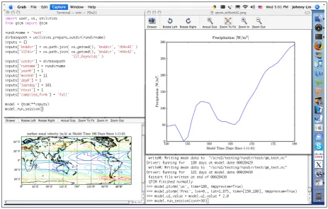
Fig. 7. Screenshot of an interactive modeling session using theqtcmpackage. The upper-left panel shows the source code file specifying the run. The lower-right panel shows the Python interpreter session making the run. The two plot windows display the plots generated by theplotmcalls from the Python interpreter command line.
instance methodvarinit, also without input parameters in the calling argument list. The fourth element of the run list is a Fortran subroutine, but with one input parameter in its calling argument list. The final routine is not a routine at all, but another run list. Regardless of what kind of routine or run list is specified, the syntax is still the same: a string or a one-element dictionary with a string as the key. Lin (2008) gives details about run lists.
3.9 Output, visualization, and analysis
The Qtcm model instance writes instantaneous and mean output to netCDF files. The netCDF data format is a plat-form independent binary plat-format that permits metadata to be saved with the data. There are a number of packages for
Python that can read and manipulate netCDF data, such as the Climate Data Analysis Tools (PCMDI, 2006).
The Matplotlib package (Hunter and Dale, 2007) for Python generates 1-D and 2-D plots using Matlab-like syn-tax. Qtcm instances have a method plotm which reads the netCDF output files and uses Matplotlib to create line or contour plots of user-specified slices of the data. Figure 7 shows an interactive modeling session with theqtcm pack-age where the user has created visualizations of a variety of parameters at run time.
Table 2. Wall-clock times (sec) for the average of three 365 day
aquaplanet runs using climatological sea surface temperature as the lower boundary forcing (Lin, 2008). All runs are executed as single threads. The “Pure” column refers to runs using the pure-Fortran QTCM1, while “Wrap” refers to the Python wrappedqtcm pack-age (v0.1.1) withcompiled form = ’parts’.
System Pure Wrap
Mac OS X: MacBook 1.83 GHz Intel Core Duo running Mac OS X 10.4.10.
152.59 158.94
Ubuntu GNU/Linux: Dell PowerEdge 860 with 2.66 GHz Quad Core In-tel Xeon processors (64 bit) running Ubuntu 8.04.1 LTS.
43.73 47.45
time. This enables the user to utilize the powerful analysis tools provided by the Climate Data Analysis Tools, SciPy (van der Walt, 2008), and other Python packages, during as well as after run time.
3.10 Model performance
Because the model’s core numerics are written in Fortran, with Python providing a sophisticated programmer/user-interface, the performance penalty of the qtcm pack-age (withcompiled form = ’parts’), compared to the pure-Fortran QTCM1 is approximately 4–9% (the penalty for compiled form = ’full’ is less). Table 2 gives wall-clock values forqtcmrunning on two platforms, Mac OS X and Ubuntu GNU/Linux.
4 Example uses of theqtcmpackage
By wrapping the Fortran QTCM1 with a Python layer, the qtcmpackage permits us to accomplish science tasks that would otherwise require a labyrinthine set of shell scripts, temporary input and output files, and source code versions. In this section, we describe a few such science tasks to il-lustrate what the Python wrapping buys us. The examples in this section are taken from Lin (2008).
4.1 Conditionally explore parameter space
Figure 8 provides an example of code that explores differ-ent values of mixed-layer depth (ziml) over a set of 30 day runs, as a function of maximum zonal wind associated with the first baroclinic mode (u1) magnitude, until it finds a case where the maximum ofu1is greater than 10 m/s. (The re-lationship betweenzimland the maximum of the speed of u1, whereziml = 0.1 * maxu1, is made up.) With each iteration, the new run uses the snapshot from a previous run as its initialization (as well as the new value ofziml); the try statement is used to ensure the model works even if
mysnapshotis not defined (which is the case the first time around).
If we implemented this science task using the pure-Fortran QTCM1 and shell scripts, we would probably have to write a separate program (possibly in a separate data analysis lan-guage like IDL, Matlab, or NCL) to analyze model output. Required parameters might be passed through an operating system pipe, or through namelists and temporary files. Au-tomating modeling with analysis in such an environment can be difficult, limited, and error prone. Theqtcmpackage al-lows us to take advantage of Python’s numerical computing capabilities so that we can embed our traverse of parame-ter space within awhileloop, thus automating the analysis task within the modeling environment.
4.2 Test alternative parameterizations
Figure 9 demonstrates the following scenario. Assume we have nine different cloud physics schemes we wish to test in nine different runs. The easiest way to do this is to take advantage of Python’s object-oriented inheritance ca-pabilities, creating a new class NewQtcmthat inherits ev-erything from Qtcm, and to which we add the additional cloud schemes (cloud0,cloud1, etc.). In theforloop in Fig. 9, we change the cloud model run list entry in the ’atm physics1’run list to whatever the cloud model is at this point in the loop.
Of course, we could do the same thing by running the nine models separately, but this set-up makes it easy to do hy-pothesis testing between these nine models as the models are running. For instance, we can create a test by which we will choose which of the nine models to use: Within this frame-work, the selection of those models can be altered by chang-ing a strchang-ing. If the same task were implemented with shell scripts and makefiles, we would have to write our own lector routines (perhaps using file system functions) for se-lecting model(s) from amongst the possible executables. It is much easier to use Python’s built-in string manipulation routines.
5 Discussion and conclusions
In the present work, an intermediate-level atmosphere model written in Fortran is wrapped with an object-oriented struc-ture written in Python, which makes modern data abstraction utilities available to a model written in a traditional proce-dural language. The result is a model that can be used dy-namically at run time, with the user able to change the order of subroutine execution at will, and able to analyze model results within the modeling environment.
import os
import numpy as N maxu1 = 0.0
while maxu1 < 10.0: iziml = 0.1 * maxu1
iname = ’ziml-’ + str(iziml) + ’m’ ipath = os.path.join(’proc’, iname) os.makedirs(ipath)
model = Qtcm(**inputs) try:
model.sync set py values to snapshot(snapshot=mysnapshot) model.init with instance state = True
except:
model.init with instance state = False model.ziml.value = iziml
model.runname.value = iname model.outdir.value = ipath model.run session()
maxu1 = N.max(N.abs(model.u1.value)) mysnapshot = model.snapshot
del model
Fig. 8. Example of an exploration of the effects of different values of mixed-layer depth. Theinputsdictionary is initialized similarly as in Fig. 1.
import os
class NewQtcm(Qtcm): def cloud0(self):
[...]
def cloud1(self): [...]
def cloud2(self): [...]
[...]
inputs[’init with instance state’] = False for i in xrange(10):
iname = ’cloudscheme-’ + str(i) ipath = os.path.join(’proc’, iname) os.makedirs(ipath)
model = NewQtcm(**inputs)
model.runlists[’atm physics1’][1] = ’cloud’ + str(i) model.runname.value = iname
model.outdir.value = ipath model.run session()
del model
Fig. 9. Example of using inheritance in Python to explore the effects of multiple cloud physics schemes in multiple runs. The[...]denote the code of the different (hypothetical) cloud physics schemes. Theinputsdictionary is defined similarly as in Fig. 1.
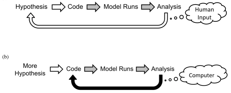
sequence with more capabilities. The traditional sequence begins with formulation of a hypothesis, then leads to im-plementing a test of the hypothesis in model code, making model runs using the coded test, and ends with analyzing the model results using various statistical and visualization packages (Fig. 10a). Some transitions between the various steps mainly make use of human input (e.g., from
(a)
Hypothesis Code Model Runs Analysis Human Input
(b)
More
Hypothesis Code Model Runs Analysis Computer
Fig. 10. Schematic of (a) the traditional analysis sequence used in modeling studies, and (b) the transformed analysis sequence using
qtcm-like modeling tools. Outlined arrows with no fill represent mainly human input. Gray-filled arrows represent a mix of human and computer-controlled input. Completely filled (black)-arrows represent purely computer-controlled input.
In contrast, the tools provided byqtcmand similar pack-ages open up the potential to automate substantially larger portions of the analysis sequence. Figure 10b shows a schematic of how model analysis might be transformed. In-stead of being limited to a few hypotheses, the transformed sequence makes additional types of hypotheses accessible without changing the complexity of the code required (see Sect. 4’s examples as illustrations). Most importantly, the Fig. 10b sequence enables model output analysis to automat-ically control future model runs. Instead of requiring human intervention to determine future model runs, the computer can make that evaluation, and as a result, for the same com-plexity of code, we can more intelligently explore the prob-lem’s solution space.
Thus, though the use of mixed language programming en-vironments for climate modeling has a modest cost in perfor-mance, these environments have the potential the pay back substantial dividends in code simplicity, reliability, and ease-of-use. More importantly, such an environment, by provid-ing a robust programmprovid-ing interface with capabilities tradi-tional languages cannot easily support, gives researchers the tools to investigate previously inaccessible (or difficult to ac-cess) questions. The wrapping techniques illustrated in the present study for the Neelin-Zeng QTCM1 may be fruitfully deployed to other climate models, increasing their flexibility and scientific usefulness.
Acknowledgements. Thanks to David Neelin, Ning Zeng,
Matthias Munnich, and the Climate Systems Interactions Group at UCLA for encouragement and help. Thanks to Alexis Zubrow, Christian Dieterich, Rodrigo Caballero, Michael Tobis, and Ray Pierrehumbert for Python help. Comments by reviewers Charles Doutriaux and Sebastien Denvil were very helpful. Early development ofqtcmprecursors was carried out at the University of Chicago Climate Systems Center, funded by the National Science Foundation (NSF) Information Technology Research
Program under grant ATM-0121028. Any opinions, findings and conclusions or recommendations expressed in this material are those of the author and do not necessarily reflect the views of the NSF. Trademarks in the present work are the property of their respective owners.
Edited by: O. Marti
References
Beazley, D. M.: SWIG 1.1 Users Manual, http://www.swig.org/ Doc1.1/HTML/Contents.html, 1997.
Edwards, P. N.: A brief history of atmospheric general circulation modeling, in: General Circulation Development, Past Present and Future: The Proceedings of a Symposium in Honor of Akio Arakawa, edited by: Randall, D. A., Academic Press, New York, 67–90, 2000.
Gushchina, D., Dewitte, B., and Illig, S.: Remote ENSO forcing versus local air-sea interaction in QTCM: A sensitivity study to intraseasonal variability, Adv. Geosci., 6, 289–297, 2006, http://www.adv-geosci.net/6/289/2006/.
Hunter, J. and Dale, D.: The Matplotlib User’s Guide, http:// matplotlib.sourceforge.net/users guide 0.98.1.pdf, 2007. Johnson, R. A.: Object-oriented analysis and design – What does
the research say?, J. Comput. Inform. Syst., 42, 11–15, 2002. Lin, J. W.-B.: qtcm User’s Guide, http://www.johnny-lin.com/py
pkgs/qtcm/doc/manual.pdf, 2008.
Lin, J. W.-B. and Neelin, J. D.: Influence of a stochastic moist convective parameterization on tropical climate variability, Geo-phys. Res. Lett., 27, 3691–3694, 2000.
Lin, J. W.-B. and Neelin, J. D.: Considerations for stochastic con-vective parameterization, J. Atmos. Sci., 59, 959–975, 2002. Lin, J. W.-B., Neelin, J. D., and Zeng, N.: Maintenance of tropical
intraseasonal variability: Impact of evaporation-wind feedback and midlatitude storms, J. Atmos. Sci., 57, 2793–2823, 2000. Mesinger, F. and Arakawa, A.: Numerical Methods Used in
Neelin, J. D. and Zeng, N.: A quasi-equilibrium tropical circulation model – formulation, J. Atmos. Sci., 57, 1741–1766, 2000. Neelin, J. D., Zeng, N., Chou, C., Lin, J., Su, H.,
Munnich, M., Hales, K., and Meyerson, J.: The Neelin-Zeng Quasi-Equilibrium Tropical Circulation Model (QTCM1), Ver-sion 2.3, UCLA Department of Atmospheric Sciences, Los Angeles, http://www.atmos.ucla.edu/∼csi/qtcm man/v2.3/qtcm manv2.3.pdf, 2002.
Oliphant, T. E.: Python for scientific computing, Comput. Sci. Eng., 9, 10–20, 2007.
PCMDI: Climate Data Analysis Tools, http://cdat.sf.net, 2006. Pennington, N., Lee, A. Y., and Rehder, B.: Cognitive activities
and levels of abstraction in procedural and object-oriented de-sign, Hum.-Comput. Interact., 10, 171–226, 1995.
Peterson, P.: F2PY Users Guide and Reference Manual, http://cens. ioc.ee/projects/f2py2e/usersguide/index.html, 2005.
PyCCSM: pyccsm: A Python version of the CCSM coupler, http: //code.google.com/p/pyccsm/, 2008.
Unidata: The NetCDF Tutorial, Boulder, CO, http://www.unidata. ucar.edu/software/netcdf/docs/netcdf-tutorial.html, 2007. van der Walt, S.: Documentation: NumPy and SciPy, http://www.
scipy.org/Documentation, 2008.
van Rossum, G.: Python Tutorial: Release 2.5.2, Python Software Foundation, http://www.python.org/doc/2.5.2/tut/tut.html, 2008. Zeng, N., Neelin, J. D., Lau, K.-M., and Tucker, C. J.: Enhancement of interdecadal climate variability in the Sahel by vegetation in-teraction, Science, 286, 1537–1540, 1999.