www.geosci-model-dev.net/4/785/2011/ doi:10.5194/gmd-4-785-2011
© Author(s) 2011. CC Attribution 3.0 License.
Geoscientific
Model Development
iGen 0.1: a program for the automated generation of models and
parameterisations
D. F. Tang1and S. Dobbie2
1School of Mathematics, University of Manchester, Manchester, UK 2School of Earth and Environment, University of Leeds, Leeds, UK
Received: 10 March 2011 – Published in Geosci. Model Dev. Discuss.: 8 April 2011 Revised: 31 August 2011 – Accepted: 31 August 2011 – Published: 16 September 2011
Abstract. Complex physical systems can often be simulated
using very high resolution models but this is not always prac-tical because of computational restrictions. In this case the model must be simplified or parameterised in order to make it computationally tractable. A parameterised model is created using an ad-hoc selection of techniques which range from the formal to the purely intuitive, and as a result it is very diffi-cult to objectively quantify the fidelity of the model to the physical system. It is rare that a parameterised model can be formally shown to simulate a physical system to within some bounded error. Here we introduce a new approach to param-eterising models which allows error to be formally bounded. The approach makes use of a newly developed computer pro-gram, which we call iGen, that analyses the source code of a high-resolution model and formally derives a much faster, parameterised model that closely approximates the original, reporting bounds on the error introduced by any approxima-tions. These error bounds can be used to formally justify conclusions about a physical system based on observations of the model’s behaviour. Using increasingly complex phys-ical systems as examples we illustrate that iGen has the abil-ity to produce parameterisations that run typically orders of magnitude faster than the underlying, high-resolution mod-els from which they are derived.
1 Introduction
When we perform numerical experiments it is our duty, as scientists, to ensure that the computer models we use are plausible simulations of the physical systems of interest; that is, we must ensure that observation of the behaviour of the model can justifiably lead to beliefs about the physical
Correspondence to: D. F. Tang ([email protected])
system being modelled. Only then can we make scientific conclusions about physical systems based on the results of numerical experiments.
Establishing the plausibility of a model, especially a very complex one such as a climate model, is far from straight-forward (Winsberg, 2001). The fourth assessment report of the IPCC (IPCC, 2007), for example, devotes a considerable amount of space to establishing the plausibility of climate models. The IPCC report presents a number of arguments, but to turn these arguments into a plausibility for a model re-quires us to weigh up many factors and make a number of subjective judgements. For this reason, these arguments can-not be used to make a formal, objective quantification of a model’s plausibility. The arguments can be categorised into three types:
The first type of argument consists of comparing the out-put of a model to data from experiment, high-resolution sim-ulation or a model from another research group. When as-sessing the plausibility of a model based on this type of ar-gument we must consider how much (or little) of the phase space of the model has been shown to be similar to the data. Based on this, it is difficult to prove that the untested por-tions of the phase space also have small error. It could be, for example, that these similarities can be explained, at least partially, by the tweaking and tuning of the model. When the data is experimental we must consider its limited precision and incompleteness: how was a complete set of boundary conditions for the simulation constructed and how was the model output compared to the data? When the data comes from other simulations we must assess, in turn, how plausi-ble those simulations are.
786 D. F. Tang and S. Dobbie: iGen 0.1: a program for automatic parameterisation The third type of argument presents an account of how the
model, or its constituent parts, are related to the underlying physics of the system of interest through a set of simplifi-cations, idealisations, approximations and established mod-elling techniques. If each of these techniques is plausible, it is argued, then the resulting model is also plausible. Typical simplification techniques include:
– Neglect of some physical process: sometimes a physical
process we know to be present in the physical system is not included in the model. Sometimes the error can be formally shown to be insignificant (e.g. neglect of the height dependence of gravitational acceleration), other times we must appeal to our physical intuition (e.g. ne-glect of the carbon cycle in a climate model).
– Idealisation: sometimes a model is based on
assump-tions we know to be false (e.g. that the sea has the vis-cosity of honey or that light travels only vertically) in or-der to make it easier (or, sometimes, possible) to or-derive the equations of the system. Quite often we do not have an exact physical description of the system, so there is no way to quantify the error introduced by the idealisa-tion. We must then appeal to our physical intuition to assess whether the idealisation will effect the behaviour of the model in a way that we care about.
– Empirical/Semi-Empirical parameterisation: when our
physical understanding does not provide us with a set of equations to describe a physical process, model building is guided in an ad-hoc and informal way by a combina-tion of theory, physical intuicombina-tion, idealisacombina-tion, experi-mental data and a certain amount of trial and error. Since these arguments cannot lead to an objective quantifica-tion of a model’s plausibility, we must rely on the judgement of the scientific community to weigh up the various argu-ments and give an inter-subjective quantification. This state of affairs has, without doubt, produced many good models and useful scientific results, but on more than one occasion it has produced conclusions that are somewhat clouded by questions of the model’s plausibility.
iGen presents a new method of generating parameterisa-tions of complex physical systems whose underlying equa-tions of motion are known. The generated parameterisaequa-tions have formally bounded error, allowing their plausibility to be objectively established. The method begins with a model of sufficiently high resolution to resolve all the relevant physical processes. Knowledge of the behaviour of this model can jus-tifiably lead to beliefs about the physical system since by def-inition the model integrates the underlying equations of mo-tion with sufficient accuracy. However, such high-resolumo-tion models would run far too slowly to be considered to be prac-tical models or parameterisations. Suppose, though, that we view the high-resolution model as a formal definition of the desired behaviour of the parameterisation, rather than a code
to be executed. The problem of parameterisation then re-duces to one of finding a computer program that closely ap-proximates the behaviour of the high-resolution model but uses far fewer computational operations. This is where iGen comes in. iGen takes as input the source code of the high-resolution model. Rather than execute it, iGen analyses the structure of the code, applies appropriate approximations, de-rives the source code of a faster model and reports bounds on the error between the fast model and the high-resolution model. Because the parameterisation is formally derived from the high-resolution model, with bounded error, its out-put can be used to justify conclusions about the behaviour of the high-resolution model, and so about the physical system of interest.
As an illustration of this method, take the problem of the parameterisation of deep convection. One so-lution to this problem is to replace the parameterisa-tion with a high-resoluparameterisa-tion model that resolves the con-vection, this is the idea behind superparameterisation (Grabowski and Smolarkiewicz, 1999). However, superpa-rameterisations are computationally very expensive. iGen goes one step further by analysing the source code of the superparameterisation and deriving a much more computa-tionally efficient model which provably approximates the su-perparameterisation with a specified error bound.
iGen can also be used as a tool for exploring the behaviour of high-resolution models. Traditionally, a numerical exper-iment would consist of executing a model with one or more input values to get one or more corresponding output values. iGen offers an alternative type of numerical experiment in which the model is formally analysed to extract functional relationships between large-scale observables. If we are try-ing to understand the emergent behaviour of a complex sys-tem, a formally derived functional relationship between ob-servables is of much more immediate use to us than a set of input/output pairs. For example, if we propose a theory that predicts some relationship between observables, then iGen’s analysis of the high-resolution model could supply us with a formal derivation of this relationship from the underlying equations of motion. Alternatively, we may not yet have a fully formed theory, but the discovery of a simple functional relationship between observables would be a valuable piece of evidence that informs and directs our theory building ef-forts. Held (2005) discusses how we could come to under-stand a very complex physical system by building a hierarchy of models, each one simpler than the last as conceptual com-plications are peeled away in sequence like layers from an onion. iGen could be used in the development of such a hier-archy by demonstrating formal links between models, testing hypothetical links and exploring our incomplete theories.
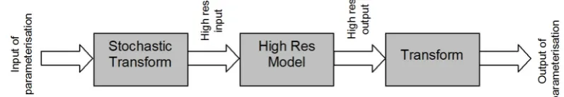
Fig. 1. Schematic of a wrapped, high-resolution model.
2 Description of the method
The proposed method can conveniently be split into four steps as follows:
1. Write a high-resolution model of the physical system of interest.
2. Define the inputs and outputs of the parameterisation and the range of inputs over which the parameterisation should be valid.
3. “Wrap” the high-resolution model.
4. Feed the source code of the wrapped model into iGen. The first step is to write a high-resolution model of the physical system. This should be of high enough resolution to ensure that the model captures all the behaviour that is of interest to us. The next step is to define the inputs and outputs of the parameterisation. In general, the inputs to the parameterisation will be some coarse-grained descrip-tion of the system which contains much less detail than the input to the high-resolution model. Equally, the output of the parameterisation will generally be some large scale or coarse-grained observable, rather than the detailed output of the high-resolution model. The range of values over which these inputs should be valid should also be decided upon at this stage. This could be based on the physically meaningful range of each input, on theoretical bounds or on some set of observed or simulated historical data.
The next step is to “wrap” the high-resolution model so that its inputs and outputs are those of the desired parame-terisation as defined in the previous step. The idea here is to turn the high-resolution model into a (very slow) param-eterisation, something akin to a superparameterisation. To do this, two pieces of extra code should be written to trans-form the inputs and outputs of the model. The first piece of code should take a coarse-grained input of the param-eterisation and transform it into a start state of the high-resolution model. Since the input to the parameterisation may not uniquely specify a high-resolution start state, a ran-dom number generator may be used to choose between pos-sible states. The code should be written so that the proba-bility of returning a high-resolution stateψon inputxis the conditional probability of finding the system in stateψgiven
that it conforms to the coarse-grained descriptionx. How difficult this is depends on the nature of the model and the desired parameterisation. In some cases a simple, uniform probability distribution may suffice, in others the distribution may be based on experimental data or the result of some kind of constrained spin-up that allows the system to settle onto its attractor. The range of values that each input can take is also specified in this piece of code by including arange di-rective that is read by iGen during the analysis. The second piece of extra code should extract the desired output from the high-resolution output. This is usually quite straightforward. So, the wrapped model should take a coarse-grained input, transform it stochastically into a high-resolution state, pass it through the high-resolution model and finally extract the output of interest (see Fig. 1).
Once the model is wrapped, its source code can be fed di-rectly into iGen together with a limit on the acceptable error in the parameterisation. iGen then analyses the code, “in-tegrates over” any random numbers, applies approximations and outputs an alternative code and a set of error bounds. The output of iGen is the source code of an efficient param-eterisation and the bounds give us formally derived bounds on the error between the parameterisation and the wrapped, high-resolution model.
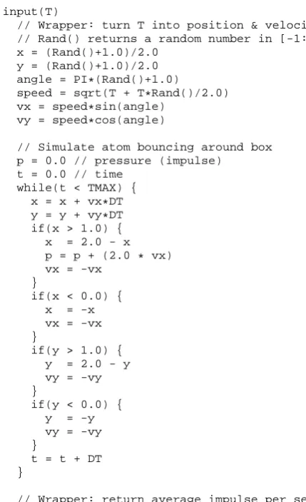
To illustrate this technique consider a simulation of a gas contained within a 2-dimensional box and suppose that we wish to parameterise the pressure of the gas in terms of its temperature. In this case, the high-resolution model is a sim-ulation of an atom bouncing around a box of unit dimen-sion. To wrap the model we extract the pressure by calcu-lating the average impulse per second on the right hand wall of the box and use this as output. The input is the temper-ature which is proportional to the average kinetic energy of the atom (for simplicity we assume a uniform distribution of kinetic energy rather than the Maxwell-Boltzmann distribu-tion, but this does not affect the result). The initial velocity, position and direction of motion of the atom is chosen at ran-dom using a ranran-dom number generator. The pseudocode for the program is shown in Fig. 2.
788 D. F. Tang and S. Dobbie: iGen 0.1: a program for automatic parameterisation
4
D. F. Tang and S. Dobbie: iGen: a program for automatic parameterisation
input(T)
// Wrapper: turn T into position & velocity // Rand() returns a random number in [-1:1] x = (Rand()+1.0)/2.0
y = (Rand()+1.0)/2.0 angle = PI*(Rand()+1.0)
speed = sqrt(T + T*Rand()/2.0) vx = speed*sin(angle)
vy = speed*cos(angle)
// Simulate atom bouncing around box p = 0.0 // pressure (impulse)
t = 0.0 // time while(t < TMAX) {
x = x + vx*DT y = y + vy*DT if(x > 1.0) { x = 2.0 - x p = p + (2.0 * vx) vx = -vx
}
if(x < 0.0) { x = -x vx = -vx }
if(y > 1.0) { y = 2.0 - y vy = -vy }
if(y < 0.0) { y = -y vy = -vy }
t = t + DT }
// Wrapper: return average impulse per sec p = p/TMAX
output(p)
Fig. 2.
Program to simulate an atom bouncing around a
2-dimensional box.
3
Symbolic analysis
iGen works by using the technique of “symbolic analysis”
(Fahringer and Scholz, 2003) in which the variables of the
program are not considered to be floating point numbers with
specific values but instead are considered to be symbolic
ex-pressions that are functions of the program’s input variables.
iGen represents variables as pairs
(C,b)
where
C
is a
mul-tivariate polynomial and
b
is a constant bound on the error
in
C
due to any approximations that have been applied. We
call these pairs “polynomial bounds”. In the following
sec-tions we explain how the structures encountered in a typical
programming language can be interpreted in terms of
poly-nomial bounds.
3.1
Arithmetic
Suppose we wish to generate an approximation of the very
simple program
input(x)
a = x + 1.0
y = a*a
y = y*y
output(y)
for inputs in the range
−
0
.
1
≤
x
≤
0
.
1.
Geosci. Model Dev., 4, 1–12, 2011
www.geosci-model-dev.net/4/1/2011/
Fig. 2. Program to simulate an atom bouncing around a 2-dimensional box.
the thermodynamic relationshipp∝T of an ideal gas from the underlying equations of kinetic theory.
3 Symbolic analysis
iGen works by using the technique of “symbolic analysis” (Fahringer and Scholz, 2003) in which the variables of the program are not considered to be floating point numbers with specific values but instead are considered to be symbolic ex-pressions that are functions of the program’s input variables. iGen represents variables as pairs(C,b)whereC is a mul-tivariate polynomial andbis a constant bound on the error inCdue to any approximations that have been applied. We call these pairs “polynomial bounds”. In the following sec-tions we explain how the structures encountered in a typical programming language can be interpreted in terms of poly-nomial bounds.
3.1 Arithmetic
Suppose we wish to generate an approximation of the very simple program
input(x) a = x + 1.0 y = a*a y = y*y output(y)
for inputs in the range−0.1≤x≤0.1.
Normally, we would simply execute this program for some input, say x=0.1. So, after the first line a=1.1, af-ter the second liney=1.1×1.1=1.21, the next liney=
1.21×1.21=1.4641 and the output would be 1.4641. How-ever, when analysing the program the input value is not spec-ified. Instead, the input,x, is treated as the polynomial bound
(x,0.0)and the program is interpreted as a sequence of arith-metic operations on polynomial bounds.
Arithmetic on polynomial bounds is interpreted in the fol-lowing way:
(P ,1)+(Q,2)→(P+Q,1+2)
(P ,1)−(Q,2)→(P−Q,1+2)
(P ,1)×(Q,2)→(P×Q,B(P )2+B(Q)1+12)
(R,)−1→
R−1,BR−12
whereB(P )is a constant bound on the absolute value ofP
over the domain of inputs. Here, the rule for finding the re-ciprocal makes use of the inequalityB(P2)≤B(P )2.
Let’s now analyse the example program above using this definition of arithmetic. The first line setsato(1+x,0.0), the second line setsyto(1+2x+x2,0.0), after the next line
y becomes(1+4x+6x2+4x3+x4,0.0)so the output of the program is the polynomial bound(1+4x+6x2+4x3+
x4,0.0). If we evaluate this polynomial atx=0.1, for exam-ple, we get 1+0.4+0.06+0.004+0.0001=1.4641, as we would expect.
An implementation of this analysis process can increase the speed of the analysis, and of the resulting model, by ap-plying approximations that reduce the degree of the polyno-mial bound.This can be formalised as the rule
(P±δ,)→(P ,+B(δ)) .
For example, suppose we are willing to accept errors in the output of our example program up to an absolute value of 0.04. The program’s symbolic output can be expanded in the Chebyshev basis as (0.0000125T4(x0)+0.001T3(x0)+ 0.03005T2(x0)+0.403T1(x0)+1.03004,0.0)whereTn(x0)is
thenth Chebyshev polynomial and we use the normalisation
x0=10x so that the independent variable lies in the range
−1≤x0≤1. This can be approximated by simply truncat-ing the appropriate number of higher order Chebyshev terms, giving(0.403T1(x0)+1.03004,0.0310625), where the bound is calculated using the inequality|Tn(x)| ≤1.0. This can
eas-ily be turned back into the program
input(x)
y = 4.03*x + 1.03004 output(y)
which approximates the original program given at the start of this section with an error bounded by±0.0310625 and reduces the number of computational operations from 3 to 2.
3.2 Random numbers
As mentioned in the introduction, when we wrap the high-resolution model the transformation from low-res input to high-res input will generally make use of a random num-ber generator. To generate random numnum-bers the wrapped model should call a function, rand(), which, upon exe-cution, returns a random floating point number with uniform probability over the range(−1:1). When analysing a call torand(), iGen generates a unique, especially tagged vari-able. The moments of each output can then be calculated by integrating over each of the tagged variables. For example, take the program
input(x)
x = x + 0.005*rand() a = x + 1
y = a*a y = y*y output(y)
The first moment of the output,y, would be
¯
y=1
2
R1
−1
(1+4x+6x2+4x3+x4)+
(0.02+0.06x+0.06x2+0.02x3)r0+
(0.00015+0.0003x+0.00015x2)r02+
(5×10−07+5×10−07x)r03+6.25×10⁻¹⁰r04dr0 wherer0is the output of the random number generator. Since the outputs are always expressed in polynomial form, iGen can use a simple algorithm to integrate them symbolically. Evaluating this integral gives
¯
y=1.000050000125+4.0001x+6.00005x2+4x3+x4.
3.3 Fixed loops
A loop with a fixed number of iterations can be expressed as the composition of a vector of polynomial bounds. Take, for example, the program
input(r) x = 0.0 y = 1.0 z = 0.0
loop 6 times {
dx_dt = 10.0*(y-x) dy_dt = r*x - y - x*z dz_dt = x*y - (8.0/3.0)*z x = x + dx_dt*0.01
y = y + dy_dt*0.01 z = z + dz_dt*0.01 }
output(x)
which integrates the Lorenz equations over six time-steps. The input to the program,r, is the parameterrin the Lorenz equations (Lorenz, 1963) which is a non-dimensionalised measure of the Rayleigh number, and the output of the pro-gram is the value of thex parameter after 6 timesteps. The loop can be dealt with by identifying the variables whose ini-tial values are referenced in a single iteration of the body of the loop; in this casex,y andz. Suppose these are placed into a vector of polynomial bounds
L=
(x,0.0) (y,0.0) (z,0.0)
.
A single iteration of the body of the loop can now be calcu-lated, in the usual way, as the vector
L=
(x+0.1y−0.1x,0.0) (y+0.01rx−0.01y−0.01xz,0.0)
(z+0.01xy−0.08
3 z,0.0)
.
The whole loop, then, is equal to the compositionL6(x,y,z)
and the output, x, is just the first element of this. On per-forming the composition and evaluating for the initial values
(0,1,0)forx,yandz, respectively, the output equates to
x= −1.09964×10⁻¹⁵r3+5.66995×10⁻⁷r2+
0.00169011r+0.455595.
If we specify that the input, r, lies in the range 0≤r≤28 (which includes the value used by Lorenz) and that errors up to 10−4 are acceptable, then the output can be truncated in the Chebyshev basis to give the approximation
x=0.00171r+0.45554±5.6×10⁻⁵.
This equation converts to a computer program
input(r)
x = 0.00171*r + 0.45554 output(x)
790 D. F. Tang and S. Dobbie: iGen 0.1: a program for automatic parameterisation An important point to note here is that in the previous
ex-amples the analysis has proceeded sequentially, in much the same order as it would during an execution. The loop,L6, however, illustrates that an analysis may proceed very differ-ently from an execution. During an execution of the loop, the program pointer would loop round 6 times; during an anal-ysis, on the other hand, we immediately define the mean-ing of the loop asL6. This can be evaluated in any way we please. For example, we may evaluateM=L⊗L⊗L, thenL6=M⊗M, givingL6in 3 (albeit polynomial) oper-ations. In some cases, there exists a closed form solution for a loop Ln in terms of n. As a simple example, sup-pose we have a loop with 100 iterations, and the body of the loop evaluates toL=< (2X,0.0),(Y+1,0.0) >for an input vector< X,Y >. Lncan be immediately solved as Ln=< (2nX,0.0),(Y+n,0.0) >givingL100=< (2100X,0.0),(Y+
100,0.0) >without the need to go through the 100 iterations.
So, when a program is executed, a program pointer moves, step by step, through the program. When a program is anal-ysed, however, its equivalent polynomial bound is built up from the structures of the program. There is no program pointer, structures can be transformed in any order, the end of the program may be transformed before the beginning.
3.4 ifstatements
Consider the following program which roughly simulates a ball bouncing on the floor in a gravitational field:
input(z) g = 10.0 dt = 0.01 v = 0.0
loop 100 {
z = z + v*dt - 0.5*g*dt*dt v = v - g*dt
if(z < 0) { v = -0.8*v z = 0.0 }
} output(z)
z is the height of the ball andv is its velocity in the up-ward direction. The input is the initial height that the ball is dropped from and is taken to be in the range 1≤z≤2.
The new structure here is theifstatement. This can be dealt with by using the Heaviside step function, defined as
H (x)=
1 ifx >0 0 ifx <0 whereH (0)is undefined.
The body of the if statement can be calculated in the same way as we did for fixed loops, giving the vector
P=((0.0,0.0),(−0.8v,0.0)).The meaning of the wholeif
statement can be written as an expression of the form
F=H (−z)P+H (z)I
whereI=((z,0),(v,0))is the identity vector (i.e. thenth el-ement is equal to thenth variable). To see thatF has the cor-rect meaning consider that ifz <0 thenF =P and ifz >0 thenF=I. This is exactly the behaviour we require for F to be equivalent to theifstatement1.
So, the whole loop equates to the vector
L=
(H (z+0.01v−0.0005)(z+0.01v−0.0005),0) ((1−1.8H (z+0.01v−0.0005))(v−0.1),0)
and the whole program equates toL100((z,0),(0,0)). In general, the condition in anifstatement may also con-tain conjunctions&&or disjunctions||so that(A && B)
is true if and only ifAandBare both true, and(A || B)
is true if and only ifAorBor both are true. A disjunction
(A || B)is taken to be equivalent toA+B−AB and a conjunction(A && B)is equivalent toAB.
When dealing with expressions that include the Heaviside step function, iGen first applies the following set of simple reasoning rules before the approximate expansion of the step functions into polynomial bounds.
If the argument to a step function can be proved not to cross zero then the function is replaced with 0 or 1:
H (A)=1 ifBl(A) >0
whereBl(A)is a lower bound onA.
H (A)=0 ifBu(A) <0
where Bu(A) is an upper bound on A. Lower and upper bounds on polynomials are calculated usinga0±B(A−a0), wherea0is the zero-th order coefficient ofA.
To simplify the form of complex booleans, the following identities are used whenever the left hand sides are encoun-tered:
1−H (A)=H (−A)
H (H (A)P+H (−A)Q)=H (A)H (P )+H (−A)H (Q)
if H (A)H (B)H (−C)=0
and H (−A)H (C)H (−B)=0
thenH (A)H (B)+H (−A)H (C)=H (B)H (C) .
The final identity is proved by noting that
H (A)H (B)(H (C)+H (−C))+
H (−A)H (C)(H (B)+H (−B))
=H (B)H (C)+H (A)H (B)H (−C)+
H (−A)H (C)H (−B) .
1Strictly speaking, the floating point variablezmay equal 0.0 when theifstatement is reached, in which caseFwould be a func-tion ofH (0)which is undefined. However, this is rarely a problem in practice since we can always add a small random number to the inputs to represent their inherent uncertainty. When the random numbers are integrated over, the ambiguity is removed as long asP remains finite.
This may seem like a rather arbitrary piece of reasoning, but because of the wayifstatements split the input space into two partitions, this structure was found to occur quite often. Its effect is to join together neighbouring partitions that have the same approximation.
Products of Heaviside functions of the form
H (P1)H (P2)...H (PN)
can sometimes be proved to be trivially true or false, and so replaced by 1 or 0, respectively. The problem reduces to that of deciding whether a set of inequalities on polynomials is satisfiable. We used a simple algorithm based on the Gaus-sian elimination method. The algorithm first transforms the inequalities to equalities in the following way: each Heavi-side termH (Pn)is equivalent to the inequalityPn>0. Since
Pncan be bounded above byBu(Pn)(as calculated using the
sum of its Chebyshev coefficients) then there exists ayn in
the range 0< yn≤Bu(Pn)that satisfiesPn−yn=0. If we
let
yn=
B(Pn)(1+zn)
2
thenznis in the range[−1:1]and can be treated as a normal
Chebyshev variable. This leads to a set of equalities
Pn0=Pn−
B(Pn)(1+zn)
2 =0
for all 0< n≤N.
Once in this form, the highest degree terms that occur in more than one equation can be successively removed by Gaussian elimination. At each stage, the bounds of the re-maining polynomials are checked. If any has an upper bound that is below zero or lower bound above zero, the equation cannot be satisfied and so there is no solution. An equation
Pn0was removed if it could be shown to be tautological, i.e. if it could be reduced to a formzn=QandQcould be bounded
by the interval [−1:1].
We found that this algorithm detected all instances en-countered in our example programs without becoming pro-hibitively slow. However, in the worst case, this algorithm runs in worse than exponential time so the procedure quits if the number of equalities exceeds a cutoff value. No fast algorithm for solving this problem is known, the first algo-rithm was due to Tarski (1951) but this also ran in worse than exponential time. Exponential time algorithms were found by Seidenberg (1954) and later by Collins (1975). More re-cently, a sub-exponential time algorithm has been found by Grigorev and Vorobjov (1988) but execution times remain high.
3.5 Conditional loops
Conditional loops can be implemented using the structures we have already described
while(A) { ... }
is equivalent to
loop M { if(A) {
... } }
for someM that gives the maximum number of times the
whileloop can iterate over the domain of inputs.
By insisting thatMis given a finite value we are, in effect, restricting iGen’s applicability to the subset of computer pro-grams known as “basic recursive”. These are the propro-grams that can be proved to terminate. As it turns out (Solomonoff, 2005), almost all computer programs in practical use hap-pen to compute basic recursive functions. Upon reflection, it is not surprising that numerical models can be shown to terminate: they are written that way. For example, if it was suspected that an algorithm could enter an infinite loop, this would in all practical respects be considered to be a bad algo-rithm and would be rewritten or thrown out of the model. The one exception to this is the use of randomised algorithms, some of which may technically never terminate. However, these algorithms all have the property that the probability of termination very quickly approaches 1 as the number of it-erations of some loop increases. So, by limiting the number of iterations we effectively take an algorithm with a vanish-ingly small probability of not terminating and replace it with an algorithm with a vanishingly small probability of return-ing the wrong answer. So when we come to integrate over the uncertainties in the input, as long as all outputs are finite, there is always a finiteM that ensures that the result is the correct answer with a vanishingly small error. We therefore restrict ourselves to the consideration of the basic recursive functions without fear that this will be a problem for our pro-posed application.
3.6 Arrays
Array reference and modification can be performed by rep-resenting the whole array as a single polynomial with the array’s index variable as an independent variable (multidi-mensional arrays can trivially be reduced to one di(multidi-mensional arrays by using the memory address offset as the index of each element). Suppose we have an array,A, of sizeN. Let
xnbe theNequidistant points on the interval [−1:1]
xn=
2n
N−1−1
wherenis an integer in the range 0≤n < N. The Lagrange basis polynomials on these points is defined as
ln=
Y
0≤i<N,i6=n
x−xi
xn−xi
792 D. F. Tang and S. Dobbie: iGen 0.1: a program for automatic parameterisation These polynomials have the important property thatln(xm)=
0 ifn6=mandln(xn)=1. If we letai be the value ofA[i]
for all integers 0≤i < N, then the(N−1)th degree polyno-mial
A(x)=
N−1
X
i=0
aili
has the property that for any integer 0≤j < N, A(N2−j1−
1)=ai. So an array referenceA[j]has the value
A
2
j
N−1−1
.
If we now define the bi-variate polynomialL(i,x)as
L(i,x)=
N−1
X
j=0
lj
2
i
N−1−1
lj(x)
so thatL(i,x)=li(x) for any integer 0≤i < N, then the
value of an arrayAafter an assignment operationA[i] = Yis equivalent to the polynomial
A+
Y−A
2i
N−1−1
L(i) .
4 Implementation details
iGen has been written in C++ and is, at present, only ca-pable of analysing C++ source code although work is un-derway to link iGen to the GNU compiler collection (GCC) so that it can analyse all languages that can be compiled by GCC. iGen can analyse any C++ source code although calls to pre-compiled library code, other than the<cmath> li-brary, cannot be analysed. Any arithmetic that is sensitive to machine precision or that depends on overflow or float-ing point exceptions should be avoided as this behaviour is not reproduced by the analysis. Consideration should also be given to the time it will take for iGen to analyse the model. At present, integer arithmetic (but not integer loop counting) tends to lead to slow analysis speed. Luckily this is usually quite easily avoided in models of physical systems. Another consideration is that since iGen represents each variable as a polynomial, rather than a floating point number, the mem-ory requirements of an analysis can be many times that of an execution.
iGen represents polynomials as a set of values at the Gauss-Lobatto collocation points as this allows very efficient computation of arithmetic operations. The type of polyno-mial approximation used is user specifiable and is either by truncation in the Chebyshev basis or by interpolation be-tween collocation points. We chose to use the Gauss-Lobatto collocation points because of their good convergence prop-erties (Boyd, 2001), this is extended to the multivariate case by using a generalised, adaptive sparse grid as described in Gerstner and Griebel (2003).
The analysis can be terminated when the bounds on error fall below a certain level, or when a certain amount of CPU time has been used. The rate of reduction of error as analy-sis time increases depends on the smoothness of the function calculated by the wrapped model, the smoother the function, the faster the convergence. The convergence properties of the sparse grid used by iGen have been discussed at length in the literature, see for example Gerstner and Griebel (2003), Barthelmann et al. (2000) or Bungartz and Griebel (2004) for a survey. Polynomial approximations of certain discon-tinuous functions never converge, this is known as the Gibbs phenomenon. However, discontinuities in a model can be formally removed by accounting for the finite precision of the input values. This can be done by adding a random number to each input value with a magnitude that represents the preci-sion of the input. On integrating over these random numbers, any discontinuities in the wrapped model are removed.
5 Applications of iGen
5.1 Automatic derivation of the Lorenz equations
iGen was used to analyse a high-resolution model of Rayleigh-Benard convection in a 2-dimensional, laminar, in-compressible fluid on an 80×28 grid. The model was wrapped so that the input was three variables (X,Y,Z). These were converted to a state of the fluid according to
ψ (x,z)=
√
2(1+a2)
a X sin(π ax)sin(π z)
and
θ (x,z)=
√
2Y cos(π ax)sin(π z)−Zsin(2π z)
π r
whereψ (x,z)is the stream-function,θ (x,z)is the tempera-ture perturbation,a=√1
2is the aspect ratio of the convective cells andr=28 is the non-dimensionalised Rayleigh num-ber. Similarly, the output of the high-resolution model was converted back to the(X,Y,Z)phase space by extracting the appropriate lowest modes ofψandθaccording to
X=√ 1
2(1+a2)
Z Z
ψ (x,y)sin(π ax)sin(π z) dx dz
Y=√π R
2a
Z Z
θ (x,y)cos(π ax)sin(π z) dx dz
Z= −π R
2a
Z Z
θ (x,y)sin(2π z) dx dz
The final output of the wrapped model was the average rate of change ofX,Y andZover a 0.00001s simulation.
The variables, (X,Y,Z), correspond to the variables of the Lorenz equations (Lorenz, 1963), which describe a 3-variable parameterisation of Rayleigh-Benard convection. iGen analysed the wrapped model of Rayleigh-Benard con-vection and produced the following simplified code:
input(x,y,z)
dx_dt = 9.95076*y + 9.94443*x dy_dt = -0.991175*x*z - 0.999187*y
+ 27.9712*x
dz_dt = -2.65625*z + 0.997019*x*y output(dx_dt, dy_dt, dz_dt)
which is a statement of the Lorenz equations with a slight difference (less than 0.9%) in the constants. This represents an increase in execution speed of 5 orders of magnitude com-pared to the wrapped model. The slight difference between iGen’s analysis and the Lorenz equations is attributed to the finite resolution of the grid, the finite time over which the in-tegration was performed and the accuracy of the algorithm used to solve the Poisson equation.
5.2 Mie scattering
In order to demonstrate iGen’s ability to deal with much more complex mathematical functions, a program was writ-ten to simulate the scattering of parallel light by spherical water droplets. This was done using Mie theory (Bohren and Huffman, 1998) which gives a method of solving Maxwell’s equations for parallel light incident upon a sphere, using complex spherical Bessel and Hankel functions. In order to analyse this, iGen had to deal with polynomials that spanned many orders of magnitude and included sharp peaks due to resonances, without losing precision.
The program was wrapped to calculate the scattering cross section per unit mass of water for light of wavelength 500 nm scattered by a thin layer of cloud. The cloud was made up of spherical water droplets with refractive index of 1.33+1×
10−8ı. The droplets in a cloud are not generally all of the same radius and are often assumed (Dobbie et al., 1999) to have a gamma distribution given by
P (r)=Arαe−βr
where
α= 1
ve
−3.0 and
β= 1
vere
andAis a normalisation factor,veis the relative “effective variance” of the distribution and is set to 0.172, andredefines an “effective radius” of the droplets. re was taken to be the input of the wrapped model, and defined to lie in the range 5 µm to 40 µm. The output of the wrapped model was defined to be the reciprocal of the scattering cross section per unit mass.
iGen was used to analyse this wrapped model and pro-duced the simplified model for the scattering cross section
Ksca:
0 50 100 150 200 250 300 350
5 10 15 20 25 30 35 40
Scattering cross section (m
2/kg)
droplet effective radius (µm)
Mie scattering Numerical integration Parameterised value
180 200 220 240 260 280 300 320 340
5 5.5 6 6.5 7 7.5 8
Scattering cross section (m
2/kg)
droplet effective radius (µm)
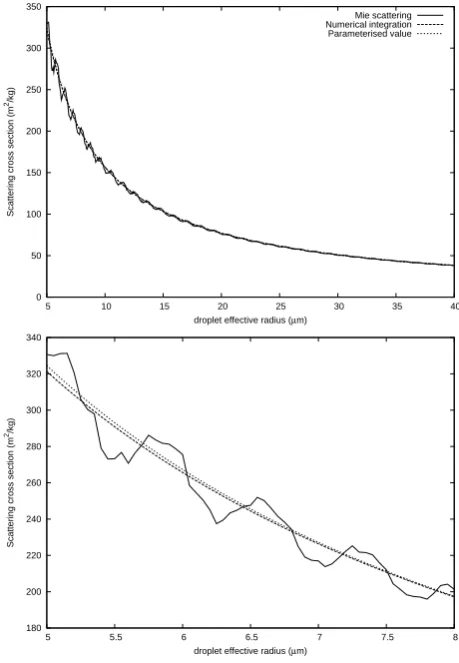
Fig. 3. Plot of scattering cross section for fixed radius droplets (solid line), numerically integrated over the droplet radius distri-bution (dashes), and iGen ’s simplified model (dots). For clarity, a magnified section is shown in the lower plot.
Ksca=
1
660.1re−2.188×10⁻⁴
with an error bounded by 4 m2kg−1. This is plotted in Fig. 3 together with the exact result calculated using numerical in-tegration.
5.3 Entrainment in stratocumulus
794 D. F. Tang and S. Dobbie: iGen 0.1: a program for automatic parameterisation The high-resolution model in this case was a
2-dimensional cloud resolving model, wrapped so that its in-put was a 5-variable specification of the large scale state of the system and the output was the mean and variance of the entrainment velocity over the final 4 h of a 6 h simulation.
iGen’s analysis produced 10th degree multivariate nomials for mean and variance of entrainment. These poly-nomials can be approximated to form a parameterisation of entrainment that executes in a few hundred arithmetic operations. iGen’s parameterisation of mean entrainment was shown to be in good agreement with data from the DYCOMS-II field campaign and from an intercomparison of cloud resolving models (Stevens et al., 2005). Full details of this experiment is given in Tang and Dobbie (2011).
6 Discussion
There remain many ways in which iGen could be developed further. iGen’s use of an adaptive sparse grid representation for polynomials goes some way to dealing with the expo-nential increase in the size of polynomial approximants as the number of independent (input) variables of the wrapped model increases. However, this “curse of dimensionality” cannot be staved off forever and iGen’s performance will quickly diminish as the number of independent variables in-creases beyond around six. The exact number of indepen-dent variables that can be practically analysed depends on the smoothness of the function calculated by the wrapped model. If the wrapped model contains many discontinuities or singu-larities then iGen’s analysis will slow down and the resulting parameterisations will have wider error bounds. This could be improved by including localised adaptive grid refinement or having a piecewise polynomial representation of variables. If the wrapped model has many more independent variables than iGen can handle then it may be possible to split the pa-rameterisation into modules and parameterise each module separately. For this to be possible each module should have inputs and outputs with clearly defined physical meaning so that wrapped models of each module can be constructed. A mathematical treatment of this strategy and a way of calcu-lating error in the whole model from the error in each module is given in Tang (2010).
If the variables in the high-resolution model become very sensitive to initial conditions then error bounds may become wide. iGen will apply approximations in order to prevent the analysis becoming too slow, and this will introduce a small uncertainty to the value of the variable. If this uncer-tainty is subsequently amplified in the final result, the error bounds will end up correspondingly wide. To improve the calculation of error bounds iGen could calculate probabilistic bounds, use bounds that are functions of the input variables or use automatic differentiation in order to apply approxima-tions more intelligently. iGen is being actively developed in this area.
It should be noted that using iGen to analyse a model is different from just fitting a curve to a model or training a neural network in two key respects. Firstly, since iGen is analysing the structure of the source code, rather than exe-cuting it, it may be possible for iGen to analyse loops in a much more computationally efficient way than executing the program multiple times on a number of input values. Sec-ondly, the analysis allows iGen to calculate error bounds that are valid over the whole of the input domain. Fitting a curve or training a neural net on a set of input/output pairs does not give any way to bound the error at points that are not in the training set without making additional assumptions about the model. So the resulting parameterisation cannot be given formally bounded error.
The iGen software and techniques described here are cur-rently being developed into a user-friendly environment that will allow scientists to use formal methods to generate mod-els of physical systems and perform numerical experiments that lead to formally provable assertions about the real world. Since the iGen source-code is changing rapidly it has not been released at this time. As soon as the iGen software reaches a stable, easy-to-use state it will be made available to the scientific community and documented in another paper. In the meantime, scientists interested in applying or experi-menting with iGen are encouraged to contact the lead author for access to the source code.
7 Conclusions
In this paper we have provided a “proof of concept” of a new technique that allows the formal generation of fast com-puter models whose error is bounded compared to a high-resolution model. This is important because it provides a for-mal, epistemic link between the results of a numerical exper-iment and the physical system that is being simulated. This ultimately allows conclusions about the physical system to be convincingly justified by the model’s output. The technique makes use of a computer program called iGen that automat-ically generates the source code of a parameterisation by analysing the source code of a high-resolution model. iGen’s ability to generate models was illustrated with a sequence of examples of increasing complexity. iGen was shown to scale up to models of realistic complexity by generating a parameterisation of entrainment in marine stratocumulus; an open problem that has been identified as a large source of uncertainty and error in existing climate models (Bony and Dufrence, 2005; Dufrence and Bony, 2008).
There is much scope for the further development of iGen and the technique described here but the authors firmly be-lieve that iGen has the potential to become an important tool for model development.
Acknowledgements. We would like to thank Zen Internet Ltd
for the loan of a computer for the stratocumulus experiment and the Natural Environment Research Council for funding this research under award number NER/S/A/2006/14148. Thanks to J. Chrimes for proof-reading this paper and supplying data for the stratocumulus experiment and to N. Stott for his discussions on polynomials. Thanks also to Wayne and Jane at North Tea Power for much needed coffee.
Edited by: I. Rutt
References
Barthelmann, V., Novak, E. and Ritter, K.: High dimensional poly-nomial interpolation on sparse grids, Adv. Comp. Maths, 12, 273–288, 2000.
Bohren, C. F. and Huffman, D. R.: Absorption and scattering of light by small particles, Wiley, New York, 1998.
Bony, S. and Dufrence, J.: Marine boundary layer clouds at the heart of tropical cloud feedback uncertainties in climate models, Geophys. Res. Lett., 32, L20806, doi:10.1029/2005GL023851, 2005.
Boyd, J. P.: Chebyshev and Fourier spectral methods, 2nd Edn., Dover publications, New York, 2001.
Bungartz, H. J. and Griebel, M.: Sparse grids, Acta Numerica, 13, 147–269, 2004.
Collins, G. E.: Quantifier elimination for real closed fields by cylin-drical algebraic decomposition, Lect. Notes Comput. Sc., 33, 134–183, 1975.
Dobbie, S., Li, J., and Chylek, P.: Two- and four-stream optical properties for water clouds and solar wavelengths, J. Geophys.-Res., 104, 2067–2079, 1999.
Dufrence, J. L. and Bony, S.: An assessment of the primary sources of spread of global warming estimates from coupled atmosphere-ocean models, J. Climate, 21, 5135–5144, 2008.
Fahringer, T. and Scholz, B.: Advanced symbolic analysis for com-pilers, Lect. Notes Comput. Sc., 2628, 1–125, 2003.
Gerstner, T. and Griebel, M.: Dimension-adaptive tensor-product quadrature, Computing, 71, 65–87, 2003.
Grabowski, W. W. and Smolarkiewicz, P. K.: CRCP: a Cloud Re-solving Convection Parameterisation for modeling the tropical convecting atmosphere, Physica D, 133, 171–178, 1999. Grigorev, D. Y. and Vorobjov, N. N.: Solving systems of polynomial
inequalities in subexponential time, J. Symb. Comput., 5, 37–64, 1988.
Held, I. M.: The gap between simulation and understanding in cli-mate modeling, B. Am. Meteorol. Soc., 86, 1609–1614, 2005. IPCC, Climate change 2007: The physical science basis.
Contribu-tion of Working Group I to the Fourth Assessment Report of the Intergovernmental Panel on Climate Change, Cambridge Univer-sity Press, Cambridge, 996 pp., 2007.
Lorenz, E. N.: Deterministic nonperiodic flow, J. Atmos. Sci., 20, 130–141, 1963.
Seidenberg, A.: A new decision method for elementary algebra, Ann. Math., 60, 365–374, 1954.
Solomonoff, R.: Algorithmic probability, AI and NKS, Lecture given at the Midwest NKS conference, 2005.
Stevens, B., Moeng, C., Ackerman, A. S., Bretherton, C. S., Chlond, A., DeRoode, S., Edwards, J., Golaz, J., Jiang, H., Khairoutdi-nov, M., Kirkpatrick, M. P., Lewellen, D. C., Lock, A., Muller, F., Stevens, D. E., Whelan, E., and Zhu, P.: Evaluation of large-eddy simulations via observations of nocturnal marine stratocumulus, Mon. Weather Rev., 133, 1443–1462, 2005.
Tang, D.: The formal generation of models for scientific simula-tions, PhD thesis, University of Leeds, 2010.
Tang, D. F. and Dobbie, S.: iGen 0.1: the automated generation of a parameterisation of entrainment in marine stratocumulus, Geosci. Model Dev., 4, 797–807, doi:10.5194/gmd-4-797-2011, 2011.
Tarski, A.: A decision method for elementary algebra and geometry, University of California Press, California, 1951.