www.geosci-model-dev.net/10/553/2017/ doi:10.5194/gmd-10-553-2017
© Author(s) 2017. CC Attribution 3.0 License.
r.avaflow v1, an advanced open-source computational framework
for the propagation and interaction of two-phase mass flows
Martin Mergili1,2, Jan-Thomas Fischer3, Julia Krenn1,4, and Shiva P. Pudasaini5
1Institute of Applied Geology, University of Natural Resources and Life Sciences (BOKU), Peter-Jordan-Straße 70,
1190 Vienna, Austria
2Geomorphological Systems and Risk Research, Department of Geography and Regional Research, University of Vienna,
Universitätsstraße 7, 1190 Vienna, Austria
3Department of Natural Hazards, Austrian Research Centre for Forests (BFW), Rennweg 1, 6020 Innsbruck, Austria 4Group Roads, Provincial Government of Lower Austria, Landhausplatz 1/17, 3109 St. Pölten, Austria
5Department of Geophysics, University of Bonn, Meckenheimer Allee 176, 53115 Bonn, Germany
Correspondence to:Martin Mergili ([email protected])
Received: 19 August 2016 – Published in Geosci. Model Dev. Discuss.: 28 September 2016 Revised: 21 December 2016 – Accepted: 5 January 2017 – Published: 6 February 2017
Abstract. r.avaflow represents an innovative open-source computational tool for routing rapid mass flows, avalanches, or process chains from a defined release area down an ar-bitrary topography to a deposition area. In contrast to most existing computational tools, r.avaflow (i) employs a two-phase, interacting solid and fluid mixture model (Pudasaini, 2012); (ii) is suitable for modelling more or less complex process chains and interactions; (iii) explicitly considers both entrainment and stopping with deposition, i.e. the change of the basal topography; (iv) allows for the definition of multi-ple release masses, and/or hydrographs; and (v) serves with built-in functionalities for validation, parameter optimiza-tion, and sensitivity analysis. r.avaflow is freely available as a raster module of the GRASS GIS software, employ-ing the programmemploy-ing languages Python and C along with the statistical software R. We exemplify the functionalities of r.avaflow by means of two sets of computational exper-iments: (1) generic process chains consisting in bulk mass and hydrograph release into a reservoir with entrainment of the dam and impact downstream; (2) the prehistoric Acheron rock avalanche, New Zealand. The simulation results are generally plausible for (1) and, after the optimization of two key parameters, reasonably in line with the corresponding observations for (2). However, we identify some potential to enhance the analytic and numerical concepts. Further, thor-ough parameter studies will be necessary in order to make r.avaflow fit for reliable forward simulations of possible fu-ture mass flow events.
1 Introduction
Rapid flows or avalanches of snow, debris, rock, or ice, or processes, process chains, or process interactions involving more than one type of movement or material, frequently lead to loss of life, property, and infrastructures in moun-tainous areas worldwide. All state-of-the-art methods for an-ticipating the occurrence, characteristics, and dynamics of such events rely on computer simulations. On the one hand, models attempt to identify those areas where mass flows are likely to release (landslide susceptibility; Guzzetti, 2006; Van Westen et al., 2006). On the other hand, they attempt to anticipate the motion of rapid mass flows once they are re-leased (Hungr et al., 2005a). Whilst conceptual models (Lied and Bakkehøi, 1980; Gamma, 2000; Wichmann and Becht, 2003; Horton et al., 2013; Mergili et al., 2015) are employed to identify possible impact areas at broad scales, physically based dynamic models are used for the detailed back-analysis or prediction of specific events.
Pitman and Le (2005), and many others (see Pudasaini and Hutter, 2007 for a review). Savage and Hutter (1989) in-troduced depth-averaged mass and momentum conservation equations which were later utilized, modified, and extended by Mangeney et al. (2003, 2005), Denlinger and Iverson (2004), and McDougall and Hungr (2004, 2005). The Sav-age and Hutter (1989) model was further extended to include the effects of pore fluid by Iverson and Denlinger (2001), Savage and Iverson (2003), Pitman and Le (2005), Pudasaini et al. (2005), Pastor et al. (2009), and Hutter and Schnei-der (2010a, b). Still, these approaches either represent effec-tively one-phase models, or do not fully consider the two-phase nature of most mass flows. More recently, the software GeoClaw and its extension D-Claw consider shallow water and quasi-two-phase flows (M. J. Berger et al., 2011; Iverson and George, 2016). Pudasaini (2012) introduced a general two-phase mass flow model including several essentially new physical aspects of two-phase solid–fluid mixture flows. In comparison to one-phase models, amongst a few other two-phase approaches (e.g. Kowalski and McElwaine, 2013), this appears suitable for the realistic simulation of most types of process chains and interactions such as overtopping of a lake and a subsequent flood or debris flow due to the impact of a landslide into the lake.
Entrainment of the basal material into the flow may sub-stantially alter the dynamics and characteristics of mass flows, increasing their destructive potential (Hungr and Evans, 2004, Hungr et al., 2005b; Reid et al., 2011; C. Berger et al., 2011; Pirulli and Pastor, 2012). Empirical laws for en-trainment were proposed by Rickenmann et al. (2003), Mc-Dougall and Hungr (2005), and Chen et al. (2006), whereas mechanical concepts were introduced by Fraccarollo and Ca-part (2002), Pitman et al. (2003a), Sovilla et al. (2006), Med-ina et al. (2008), and Iverson (2012). The available entrain-ment models are effectively single phase and developed for bulk debris (Armanini et al., 2009; Crosta et al., 2009; Hungr and McDougall, 2009; Pirulli and Pastor, 2012). Whilst the importance of erosion and the associated change of the basal topography (Fraccarollo and Capart, 2002; Hungr and Evans, 2004; Hungr et al., 2005b; Le and Pitman, 2009) have been recognized by the scientific community, attempts to sim-ulate deposition of mass flow material are sparsely docu-mented.
Various types of numerical schemes have been used to solve mass flow model equations in order to redistribute mass and momentum (e.g. Davis, 1988; Toro, 1992; Nessyahu and Tadmor, 1990; Tai et al., 2002; Wang et al., 2004). Pre-viously, equations were commonly formulated and solved for predefined types of topographies (Pudasaini et al., 2005, 2008; Wang et al., 2004), whereas a mathematically con-sistent application to arbitrary mountain topographies – and therefore to real-world conditions – still remains a chal-lenge (Mergili et al., 2012). This issue is closely related to the fact that the model equations are commonly expressed in topography-following coordinates hardly compatible with
global Cartesian coordinates, which usually appear in geo-graphic information systems (GIS) and are referred to as GIS coordinates in the following. Nevertheless, some of the mass flow models mentioned have been implemented in compu-tational tools used for hazard mapping and zoning, such as DAN (Hungr, 1995), TITAN2D (Pitman et al., 2003b; Pit-man and Le, 2005), SamosAT (Sampl and Zwinger, 2004), or RAMMS (Christen et al., 2010a, b). Hergarten and Robl (2015) developed a modelling tool relying on the open-source flow solver GERRIS (Popinet, 2009).
None of these models explicitly consider stopping and de-position, and they offer only basic functionalities for simu-lating chains or interactions of two-phase mass flows. There is, however, a particular need to appropriately consider pro-cess chains and interactions in mass flow simulations: some of the most destructive events in history have evolved from cascading effects, such as the 1970 Huascarán event in Peru (Evans et al., 2009) or the 2002 Kolka–Karmadon event in Russia (Huggel et al., 2005).
The present work addresses some of the needs and issues raised by introducing the multifunctional open-source com-putational framework r.avaflow, employing an enhanced ver-sion of the Pudasaini (2012) two-phase flow model for rout-ing mass flows from a defined release area down arbitrary to-pography to a deposition area. Next, we introduce the struc-ture and components of r.avaflow (Sect. 2). Then, we perform two computational experiments in order to demonstrate the functionalities of the computational framework (Sect. 3). We discuss the implementation of r.avaflow and the implications of our findings (Sect. 4) and finally conclude with the key messages of the work and a brief outlook on the next steps (Sect. 5).
2 The computational framework r.avaflow 2.1 Computational implementation
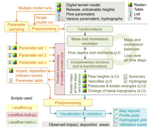
C programming language (sub-module r.avaflow.main). To-gether with Python, the R software environment for statistical computing and graphics (R Core Team, 2016) is employed for built-in validation and visualization functions. Figure 1 illustrates the logical framework of r.avaflow.
Multiple model runs may be executed in parallel, exploit-ing all computational cores available (see Sect. 2.5). This speeds up the processing considerably and allows the use of r.avaflow on computational clusters. Parallelization is imple-mented at the Python level (Mergili et al., 2014, 2015): for each model run, a batch file is produced within the module r.avaflow. This batch file calls the Python-based sub-module r.avaflow.mult, launching r.avaflow.main, which is then exe-cuted with the specific parameters for the associated model run. Thereby, the Python library “Threading”, a higher-level threading interface is exploited. The Python class “Queue” is employed for handling the queue of items to be processed.
r.avaflow was developed and tested with the operating systems (OS) Ubuntu 12.04 and 16.04 LTS, and Scientific Linux 6.6 (Red Hat). It is expected to work on other UNIX systems, too. A simple user interface is available. However, the tool may be started more efficiently through command line parameters, enabling a straightforward batching on the shell script level. This feature facilitates model testing and the combination with other GRASS GIS modules.
Experiments where parallel processing is not applied are performed on an Intel® Core i7 975 with 3.33 GHz and 16 GB RAM (DDR3, PC3-1333 MHz), exploring a maxi-mum of eight cores through hyperthreading and using the OS Ubuntu 12.04 LTS. All experiments with parallel processing are performed on the Vienna Scientific Cluster, serving with approximately 2020 nodes (Supermicro X9DRD-iF Board), each equipped with an Intel Xeon processor E5-2650v2 with 2.6 GHz and 8×8 GB RAM. The OS for these computations is Scientific Linux 6.6 (Red Hat).
2.2 Input and output
The key input parameters of r.avaflow are summarized in Table 1. Essentially, r.avaflow relies on (i) a digital terrain model (DTM) representing the elevation of the basal sur-face (in the release areas beneath the release mass) before the event under investigation, (ii) raster maps of the spatial dis-tribution of the solid and fluid release heights or hydrographs of solid and fluid release, and (iii) a set of flow parameters (Table 2). Input raster maps of the entrainable solid and fluid heights, and a raster map or value defining the empirical en-trainment coefficient (needed for enen-trainment) are optional. Instead of the solid and fluid release and entrainable heights, the total heights and fixed values of the solid concentration may be defined.
There is no restriction imposed on the arrangement of the release cells. With the term “cell”, we refer to a regular, equidistant, square, ground-projected computa-tional/numerical unit, i.e. an element of a GIS raster. Patches
Figure 1.Logical framework of r.avaflow. The transformations and retransformations refer to the conversion of heights and GIS coor-dinates to depths and topography-following coorcoor-dinates, and vice versa (see Sect. 2.3).
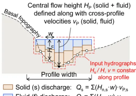
of cells where the release height is larger than zero may be defined in various parts of the investigation area. An arbi-trary number of release hydrographs – each associated with a given set of coordinates – can be defined alternatively or in addition to the release masses. This allows the simulation of complex interactions between different types of processes (see Sect. 3). Hydrographs are defined through their solid and fluid heights at the centre point of the hydrograph profiles, and by the solid and fluid flow velocities. The flow height distribution along the hydrograph profile – which should be aligned perpendicular to the main flow direction – is derived from the assumptions of a horizontal cross section of the flow table and a maximum profile length (Fig. 2).
Mandatory parameters further include the time interval at which output maps are written1tout(s), the maximum time
after which the simulation terminates, and the threshold flow height for visualization and validationHt (m; see Table 1).
Optional parameters further include raster maps of the ob-served impact area and deposition height, as well as a set of flow path coordinates (for validation and visualization; see Fig. 1 and Sect. 2.6). An exhaustive list of input parame-ters is provided in the user manual of r.avaflow, available at http://www.avaflow.org/software.html.
If a single model run is executed (see Fig. 1), the output of r.avaflow consists in raster maps of solid, fluid, and total flow heights, flow velocities inx andy direction and in ab-solute terms, pressures and kinetic energies, and the change of the basal topography (only relevant with entrainment or stopping; see Sect. 2.4). All raster maps are produced for each output time step (defined by1tout) and for the
Table 1.Key input and output parameters of r.avaflow – s: solid; f: fluid; t: total. Remarks: 1: mandatory; 2: one of the input data sets A, B, or C+D is mandatory, C+D may also be provided in addition to A or B;nD≥nC, ifnD> nCthe remaining sets of D are output hydrographs;
3: either A or B may be provided if entrainment is activated, otherwise all values ofHEmax= ∞; C is mandatory with entrainment; 4: at
least one of the data sets A, B, and C is mandatory for validation.
Parameter Symbol Unit Format Remarks
Input
Initial elevation of basal surface Z0 m Raster map 1
s, f release heights H0,s,H0,f m, m Raster maps 2A
Total release height, s concentration
of release mass H0,αs0 m, – Raster map, value 2B
s, f entrainable heights HEmax,s,HEmax,f m,m Raster maps 3A
Entrainable total height, s concentration
of entrainable mass HEmax,αs,Emax m, – Raster map, value 3B
nChydrograph tables: s and f flow heights and velocities
at defined points of time (see Fig. 2) HP,s,vP,s,HP,f,vP,f m, m s−1, m, m s−1 Tables 2C nDsets of centre coordinates, length,
and aspect of hydrograph – m, degree Sets of 4 values 2D
Flow parameters (see Table 2) – – Set of 14 values 1
Entrainment coefficient (see Table 2) CE kg−1 Value 3C
Time interval for output, max. time 1
after which simulation terminates 1tout,tterm s, s Set of 2 values 1
Threshold flow height for visualization
and validation Ht m Value 1
Observed impact area, observed deposition area OIA, ODA –, – Raster maps 4A, B
Vertex coordinates of flow path – m Even number of≥4 values 4C
Output (excluding validation and visualization output; see Sect. 2.6) Maximum flow height, kinetic energy,
and pressure (each for s, f, t) HMax,TMax,pMax m, J, Pa Raster maps Always
Flow height, flow kinetic energy, and flow pressure
at each output time steptout(each for s, f, t) Htout,Ttout,ptout m, J, Pa Raster maps Always Flow velocities inxandydirection,
and in absolute values (each for s, f) vx,vy,v m s−1 Raster maps Always
Change of basal topography (s, f, t) HC m Raster maps Always
Impact indicator index, deposition indicator index III, DII –, – Raster maps Multiple runs
nD–nCoutput hydrograph tables: flow heights, velocities,
and discharges at defined points of time (s, f) HP,vP,Q m, m s−1, m3s−1 Tables IfnD> nC
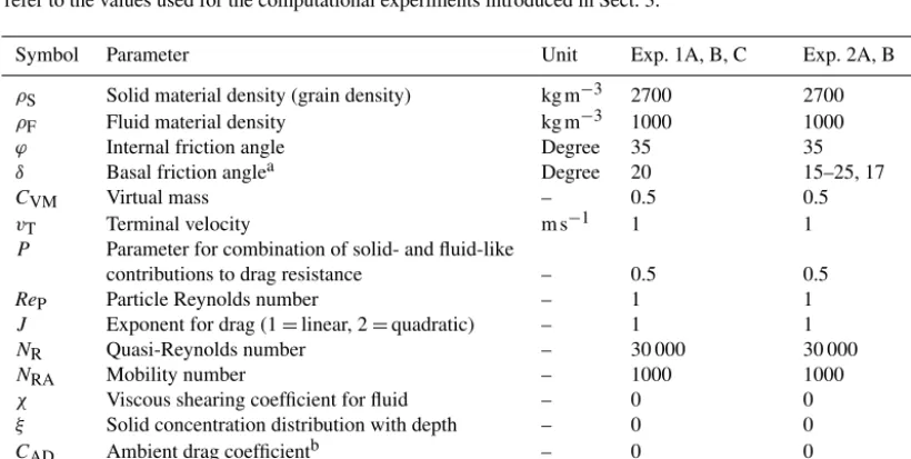
Table 2.Flow parameters and entrainment coefficient required with the enhanced version of the Pudasaini (2012) two-phase flow model. Exp. 1 and 2 refer to the values used for the computational experiments introduced in Sect. 3.
Symbol Parameter Unit Exp. 1A, B, C Exp. 2A, B
ρS Solid material density (grain density) kg m−3 2700 2700 ρF Fluid material density kg m−3 1000 1000 ϕ Internal friction angle Degree 35 35
δ Basal friction anglea Degree 20 15–25, 17
CVM Virtual mass – 0.5 0.5
vT Terminal velocity m s−1 1 1 P Parameter for combination of solid- and fluid-like
contributions to drag resistance – 0.5 0.5
ReP Particle Reynolds number – 1 1 J Exponent for drag (1=linear, 2=quadratic) – 1 1
NR Quasi-Reynolds number – 30 000 30 000 NRA Mobility number – 1000 1000 χ Viscous shearing coefficient for fluid – 0 0
ξ Solid concentration distribution with depth – 0 0
Figure 2.Sketch of a hydrograph profile. The flow surface of input hydrographs is defined byHP and is extended in cross-profile
di-rection either to the edge of the profile or until it intersects with the basal topography.
maximum solid and fluid flow heights and velocities as well as flow volumes and kinetic energies for all output time steps is produced. Optionally, solid and fluid output hydrographs are generated for an arbitrary number of given output hydro-graph profiles (see Table 1 and Fig. 2). With multiple model runs, the results of each single run are aggregated to impact or deposition indicator indices (see Sect. 2.5). In the present work, we focus on the output heights, hydrographs, and in-dices when analysing the results, rather than on velocities or deduced results such as pressures or kinetic energies (see Sect. 3).
2.3 Mass and momentum evolution
The core functionality of r.avaflow consists in the redistri-bution of mass and momentum, employing a dynamic flow model and a numerical scheme. Thereby, the tool offers im-plementations (i) of a single-phase shallow water model with Voellmy friction relation (Christen et al., 2010a, b; Fischer et al., 2012) and (ii) essentially the Pudasaini (2012) two-phase flow model with ambient drag (Kattel et al., 2016) and a set of additional numerical treatments (complemen-tary functions) outlined in Sect. 2.4. In the present work, we only consider the implementation (ii). It builds on the conser-vation of mass and momentum, computed separately but si-multaneously for the solid and fluid components of the flow. A system of six differential equations (expressed in locally topography-following coordinates) represents the basis for a set of six flux and source terms, regarding solid and fluid flow depths (Ds,Df), solid momentumMsxand fluid momentum Mfxinxdirection (Msx=Ds·vsx,Mfx=Df·vfx), andMsy andMfyinydirection (Msy=Ds·vsy,Mfy=Df·vfy), where vis flow velocity.
The Pudasaini (2012) model employs the Mohr–Coulomb plasticity for the solid stress. The fluid stress is modelled as a solid-volume, fraction-gradient-enhanced, non-Newtonian viscous stress. The generalized interfacial momentum trans-fer includes viscous drag, buoyancy, and virtual mass in-duced by relative acceleration between the phases. A new generalized drag force is proposed that covers both solid-like and fluid-solid-like contributions. Strong coupling between the solid-momentum and the fluid-momentum transfer leads to simultaneous deformation, mixing, and separation of the phases. Inclusion of the non-Newtonian viscous stresses is important in several aspects. The advection and diffusion of the solid volume fraction play an important role. The model includes a number of innovative, fundamentally new, and dominant physical aspects. Please consult Pudasaini (2012) for the full details of the model, including the corresponding equations. The flow parameters required are summarized in Table 2.
Solving the differential equations and propagating the flow from one cell to the next requires the implementation of a nu-merical scheme. For this purpose, r.avaflow employs a high-resolution total variation diminishing non-oscillatory central differencing (TVD-NOC) scheme, a numerical scheme used to avoid unphysical numerical oscillations (Nessyahu and Tadmor, 1990). Cell averages of all six state variables are computed using a staggered grid: the system is moved half of the cell size with every time step; the values at the cor-ners of the cells and in the middle of the cells are com-puted alternatively at half and full time steps, respectively. The TVD-NOC scheme with the minmod limiter has suc-cessfully been applied to a large number of mass flow prob-lems (Tai et al., 2002; Wang et al., 2004; Mergili et al., 2012; Pudasaini and Krautblatter, 2014; Kafle et al., 2016; Kattel et al., 2016).
The input and output of r.avaflow (see Sect. 2.2) is dis-cretized on the basis of GIS coordinates, i.e. in cells which are rectangular in shape in the ground projection. For the numerical solution, the cell lengths in x and y directions, and the area, are corrected for the local slope in order to maintain consistency with the state variables expressed in the local topography-following coordinates. Gravitational accel-eration in the topography-following x, y, and z directions – representing a fundamental input to the Pudasaini (2012) model equations – is computed from the DTM, employing a finite central differencing scheme. All input heightsH (m) are expressed in a vertical direction and are converted into depthsD (m) expressed in a direction normal to the local topography as in the model equation formulation. The result-ing depths are converted into heights for output. The time step length1tis dynamically updated according to the CFL condition (Courant et al., 1967; Tai et al., 2002; Wang et al., 2004).
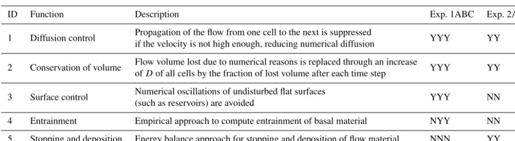
Table 3.Functionalities of r.avaflow introduced for numerical purposes (ID 1–3) or complementing the Pudasaini (2012) model (ID 4–5). Exp. 1 and 2 refer to the computational experiments introduced in Sect. 3; Y: activated, N: deactivated.
ID Function Description Exp. 1ABC Exp. 2AB 1 Diffusion control Propagation of the flow from one cell to the next is suppressed YYY YY
if the velocity is not high enough, reducing numerical diffusion
2 Conservation of volume Flow volume lost due to numerical reasons is replaced through an increase YYY YY ofDof all cells by the fraction of lost volume after each time step
3 Surface control Numerical oscillations of undisturbed flat surfaces YYY NN (such as reservoirs) are avoided
4 Entrainment Empirical approach to compute entrainment of basal material NYY NN 5 Stopping and deposition Energy balance approach for stopping and deposition of flow material NNN YY
pores in the solid material are filled with fluid (pores filled with air are excluded).
2.4 Complementary functions
Table 3 summarizes some additional functions of r.avaflow. The functions with ID 1–3 have been introduced to compen-sate for deficiencies of the numerical scheme and its imple-mentation experienced with complex real-world flows (see Sect. 4). Entrainment and stopping, in contrast, represent dy-namic functions not covered by the Pudasaini (2012) model and are executed at the end of each time step (see Fig. 1). Even though the separation of the complementary functions from the TVD-NOC scheme, and their treatment in a sim-ple forward Euler manner, can be questioned physically and mathematically, we consider the current implementation a reasonable first approximation (see Sect. 4). We now elab-orate the concepts employed for entrainment as well as for stopping and deposition in more detail.
Full handling of the evolution of the basal topography within the TVD-NOC scheme is not straightforward and could also produce some diffusion. Therefore, as entrainment is not included in the original Pudasaini (2012) model, en-trainment is treated as a complementary function in a first step. We note, however, that the time steps at which entrain-ment and the change of the basal topography are updated are identical to the time steps of the numerical scheme. The potential solid and fluid entrainment ratesqE,s andqE,f
(ex-pressed perpendicular to the basal topography) build on the user-defined empirical entrainment coefficient CE (see
Ta-ble 2) and the solid and fluid momenta. We assume a verti-cally homogeneous solid fractionαs,Emaxwithin the
entrain-able material, which is reflected in the ratio betweenqE,sand
qE,f:
qE,s =CE|Ms+Mf|αs,Emax,
qE,f =CE|Ms+Mf| 1−αs,Emax. (1)
The fact that the basal velocities, which are relevant for en-trainment, are lower than the depth-averaged velocities is not
explicitly considered, but has to be reflected in the value of CE.qE,s and qE,f are always positive. The solid and fluid
changes of the basal topography,HE,s andHE,f, due to
en-trainment are
HE,s,t=min
HE,s(t−1t )+
qE,s1t
cosβ , HEmax,s
, (2)
HE,f,t=min
HE,f(t−1t )+
qE,f1t
cosβ , HEmax,f
, (3)
where HE,s(t−1t ) and HE,f(t−1t ) are the change of
the basal topography at the start of the time step,HEmax,s
and HEmax,f are the maximum entrainable depths at the
given cell, t is the time passed at the end of the time step, 1t is the time step length, and β is the local slope of the basal surface. The division by cosβ approximates the conversion from depths to heights. The solid and fluid entrained depthsDE,s= HE,s(t )−HE,s(t−1t )cosβ and
DE,f= HE,f(t )−HE,f(t−1t )cosβ are added to the solid
and fluid flow depths. We further assume that entrainment in-creases the solid and fluid momentum of the flow in each di-rection by the product of the entrained solid and fluid depth and the velocity in the given direction (ME; Fig. 3a). The
basal topography and, consequently, thex andy cell sizes, cell areas, and gravitational acceleration components inx,y, andzdirection are updated after each time step.
The changes in gravitational acceleration also influence the magnitude of the frictional terms (Pudasaini and Hut-ter, 2003), which are important for stopping processes. In the literature, few approaches explicitly consider stopping pro-cesses directly in their numerical scheme by operator split-ting methods coupled with the determination of admissible stresses (e.g. Mangeney et al., 2003; Zhai et al., 2015). Here, in order to consider stopping which occurs at a spatial scale that is not numerically resolved, we choose a different ap-proach by proposing the dimensionless factor of mobility (FoM), relating the distance required for stopping sstop to
move-Figure 3.Interactions of the flow with the basal topography:(a) en-trainment, assuming that HEmax,s and HEmax,f are not limiting; Di: total initial flow depth (s+f); Mi: total initial momentum
(s+f);DE: entrained depth;ME: total increase in momentum due
to entrainment (s+f). Panel(b)indicates stopping and deposition. Both panels represent sections along the steepest slope of the basal topography. Note that stopping and deposition usually occur on less inclined slopes than drawn in(b)which represents upslope move-ment.
ment. The flow stops ifsstop≤1s, i.e. FoM≤1 (see Fig. 3b):
FoM=sstop
1s . (4)
To estimatesstop, we formulate the energy balance
consider-ing that the initial kinetic energy at an initial velocityv0and
the change of potential energy while travelling the distance sstophave transformed in dissipative energy due to Coulomb
friction, which dominates close to stopping. With this, the energy balance estimate yields
v20
2 +sstopsinβvg=sstoptanδcosβvg. (5) Consequently,
sstop=
v20
2gcosβv(tanδ−tanβv)
, (6)
whereδ is the basal friction angle,βvis the slope angle in
the direction of movement, and gis gravitational accelera-tion (see Table 2). According to Eq. (6) the stopping distance sstopis positive forδ > βv, meaning that stopping is possible
when the friction angle is higher than the slope angle, i.e. in particular at flat or even counter slopes. We note that, by a simple transformation of Eq. (6), FoM can alternatively be derived by relating the stopping time to the time step length. The stopping criterion is only relevant forv0>0.
FoM can relate to various spatial units, such as (i) a single cell; i.e. FoM is computed separately for each cell (it may happen that stopping of the flow occurs at a certain cell, but not at its neighbour cells); (ii)v0andβvare averaged over
a certain cell neighbourhood to compute FoM, so that stop-ping occurs at patches of adjacent cells; and (iii)βvand the
associated component ofvare averaged over the entire flow area. This means that the entire flow stops at once.
The third possibility is currently implemented with r.avaflow as an optional function. If activated, the simulation terminates as soon as stopping occurs and the entire flow ma-terial is deposited. Note that, in the current implementation, stopping and deposition always consider the total mass, with-out differentiating between the solid and the fluid compo-nents. This simplification is reasonable for flows character-ized by a relatively small fluid volume fraction. The change of basal topography due to entrainmentHEafter the last time
step is subtracted from the height of the deposited material HDin order to derive the change of basal topography (or net
deposition)HCat the end of the simulation (positive for an
increase, negative for a decrease of terrain elevation). 2.5 Multiple model runs
r.avaflow includes a built-in function to perform multiple model runs at a time with controlled or random variation of uncertain input parameters between given lower and up-per thresholds. Essentially, this concerns the flow parameters (see Table 2) but also the solid concentration of the release massαs0. Multiple parameters can be varied at a time. This
procedure serves two purposes:
– It facilitates multi-parameter sensitivity analysis and op-timization efforts.
– The results of all model runs are aggregated to an im-pact indicator index (III) and a deposition indicator in-dex (DII), each in the range 0–1. III represents the frac-tion of model runs where HMax≥Ht at a given cell,
whilst DII represents the fraction of model runs where HC≥Htat a given cell. III and DII are used to directly
account for uncertain input parameters in the simulation result.
The model runs can be assigned to multiple computational cores (parallel processing), enabling the exploitation of high-performance computational environments (see Sect. 2.1). 2.6 Validation and visualization
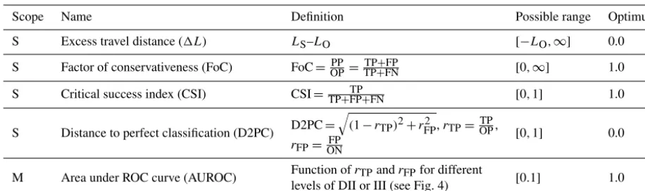
Table 4. Validation criteria used in r.avaflow (see also Fig. 4). S: single model run, binary simulation result; M: multiple model runs, simulation result in the range 0–1. The concepts of CSI and D2PC are taken from Formetta et al. (2016). All validation parameters are computed forHMax(OIA as reference) and/orHC(ODA as reference), depending on which of the reference data are available.
Scope Name Definition Possible range Optimum S Excess travel distance (1L) LS–LO [−LO,∞] 0.0
S Factor of conservativeness (FoC) FoC= PP OP=
TP+FP
TP+FN [0,∞] 1.0
S Critical success index (CSI) CSI= TP
TP+FP+FN [0,1] 1.0
S Distance to perfect classification (D2PC) D2PC=
q
(1−rTP)2+rFP2 ,rTP=OPTP, [
0,1] 0.0
rFP=ONFP
M Area under ROC curve (AUROC) Function ofrTPandrFPfor different [0.1] 1.0 levels of DII or III (see Fig. 4)
Figure 4.Validation of r.avaflow results.(a)Validation scores for single model run;(b)multiple model runs: threshold levels of III or DII, employed to produce(c)ROC curves.
at selected coordinates and time steps. Those cells with ob-served impact or deposition are referred to as obob-served pos-itives (OPs), those without observed impact or deposition as observed negatives (ONs). When using the observed impact area (OIA) as reference, all cells withHMax≥Htare
consid-ered as predicted positives (PPs), all cells with HMax< Ht
are considered as predicted negatives (PNs). When using the observed deposition area (ODA) as reference, all cells with HC≥Ht are considered as PPs, all cells withHC< Ht are
considered as PNs. Intersecting ONs and OPs with PPs and PNs results in four validation scores: true positive (TP), true negative (TN), false positive (FP), and false negative (FN) predictions (Fig. 4). TN strongly depends on the size of the area of interest. It is normalized to 5·(TP+FN)−FP in or-der to allow a meaningful comparison of model performance among different case studies. These scores build the basis for most of the validation parameters described in Table 4. Only the excess travel distance1Lrelies on the observed and sim-ulated terminal points of the flow, based on a user-defined longitudinal profile. We note that this profile is only needed
for validation but is not used for the mass flow simulation itself.
Values of1L >0 and FoC>1 indicate conservative re-sults (simulated impact or deposition area is larger than ob-served impact or deposition area) whilst values of1L <0 and FoC<1 indicate non-conservative results. CSI, D2PC, and AUROC do not allow to conclude on the conservative-ness of the results. 1L, FoC, CSI, and D2PC as defined in Table 4 target at the validation of HMax or HC derived
with one single model run. With multiple model runs (see Sect. 2.5), those validation parameters are computed sepa-rately for each run, allowing to conclude on the sensitivity of the model performance to given input parameters, or to optimize input parameter values. In this sense, optimum pa-rameters always refer to one particular criterion, and different criteria may suggest different optimum parameter values.
In contrast, ROC (receiver operating characteristic) curves are used to test the performance of the overall output of mul-tiple model runs. Such curves are produced for III (OIA as reference) and/or DII (ODA as reference): the true positive rate is plotted against the false positive rate for various levels of III or DII. The area under the curve connecting the result-ing points, AUROC, is used as an indicator for model perfor-mance (AUROC≈1 indicates an excellent performance; see Fig. 4 and Table 4).
3 Computational experiments
3.1 Experiment 1: generic process chain 3.1.1 Topographic setup
In a first step, the potential of r.avaflow for simulating pro-cess chains is demonstrated, considering the interaction be-tween one or more landslides, a reservoir, and the dam im-pounding the reservoir. This experiment represents a follow-up to the work of Pudasaini (2014), Kafle et al. (2016), and Kattel et al. (2016). We construct a generic landscape of size 3200 m×2000 m, illustrated in Fig. 5a. This landscape consists of the following elements: (i) west–east stretching trough-shaped valley with an amphitheatre-shaped head, in-clined towards the east in its lower part; (ii) dam with a trape-zoidal cross section running across the valley, consisting of 100 % solid material; (iii) reservoir impounded by the dam; (iv) landslide release mass near the northwest corner of the area of interest (Landslide 1); (v) landslide release mass di-rectly north of the dam (Landslide 2); (vi) hydrograph release of landslide near the southwest corner of the area of inter-est; (vii) measurement profile for output hydrograph down-stream from the dam. Both landslide release masses assume the shape of a distorted hemi-ellipsoid imposed on the basal topography (see Fig. 5a). The algorithm for exactly repro-ducing the generic landscape in GRASS GIS is available at http://www.avaflow.org/casestudies.html.
3.1.2 Modelling strategy and parameterization
Landslides 1 and 2 consist of 75 % solid and 25 % fluid by volume (uniformly mixed); the input hydrograph I1 (see Fig. 5b) consists of 50 % solid and 50 % fluid per volume. The parameters and settings applied are summarized in Ta-bles 2 and 3.
Three computational experiments are performed, with in-creasing complexity from A to C:
– Experiment 1A: Landslide 1 is released and interacts with the reservoir. The dam is assumed stable and may therefore not be entrained.
– Experiment 1B: Again, Landslide 1 is released and in-teracts with the reservoir. However, dam material is al-lowed to be entrained in this experiment.
– Experiment 1C: Landslide 2 is released and interacts with the dam and the reservoir. The release from the input hydrograph I1 starts after 10 s and continues for a period of 130 s (see Fig. 5). Dam material is allowed to be entrained at all stages of the computational experi-ment.
All experiments are performed at a cell size of 10 m and for a duration of tterm=300 s;1tout=5 s. The solid and fluid
Figure 5. Generic landscape used for Experiment 1A–C.
(a)Oblique view illustrating the topography and elements of the landscape.(b)Input hydrograph I1 employed for Experiment 1C.
discharges are continuously recorded at the output hydro-graph profile O1 downstream. The stopping function is de-activated (see Table 3).
3.1.3 Results
Animations illustrating the time evolution of the flow heights in all three experiments are enclosed in Animations 1A, B, and C in the Supplement.
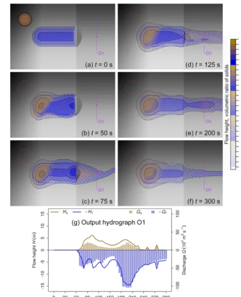
Figure 6a–f illustrates the flow heights at selected points of time during Experiment 1A. Landslide 1 (see Fig. 5a) im-pacts the backward portion of the reservoir after few sec-onds and generates a water wave – oblique and perpendicular to the impact – that overtops the dam fromt=50–55 s on-wards. The output hydrograph O1 starts recording discharge att=65 s, with the peak of the first major flood wave pass-ing att=75 s (Qf=8×10⁴m3s−1; Fig. 6g). We note that
Figure 6.Key results of Experiment 1A. (a–f)Sequence of sim-ulated flow heights and solid ratios at selected points of time; see Animation 1A in the Supplement for animations of flow height se-quences;(g)output hydrograph O1 (see Fig. 5a).
(Qf=1.5×10⁴m3s−1att=175 s;Qf=2.2×10³m3s−1at
t=285 s). The solid content passing the hydrograph profile is almost negligible as all solid landslide material remains in the reservoir basin. Att=300 s, the impact wave in the lake has almost alleviated (see Animation 1A in the Supplement). Experiment 1B (Fig. 7) is identical to the Experiment 1A until the point when the impact wave reaches the dam att= 50 s. Entrainment of the dam starts with overtopping, which sets on at the lateral portions. Part of the dam is entrained during overtopping by the initial impact wave. Whilst mas-sive outflow from the reservoir occurs due to the decreased level of the dam crest, part of the wave is deflected at the dam and pushed back towards the rear part of the reservoir, inducing a system of secondary waves. The remaining dam material is entrained when hit by those secondary waves. At t=200 s, the entire dam has disappeared and the reservoir starts emptying completely. In contrast to Experiment 1A, due to the emptying process, the system does not approach a static equilibrium aftert=300 s (see Animation 1B in the Supplement).
The temporal patterns of the simulated entrainment and wave propagation are clearly reflected in the discharge recorded at the output hydrograph O1 (see Fig. 7g). As a
Figure 7.Key results of Experiment 1B.(a–f)Sequence of sim-ulated flow heights and solid ratios at selected points of time; see Animation 1B in the Supplement for animations of flow height se-quences;(g)output hydrograph O1 (see Fig. 5a).
consequence of dam overtopping, fluid discharge at O1 starts increasing at t=65 s and reaches a first peak at t=80 s (Qf=5.1×10⁴m3). Solid discharge – a consequence of
en-trainment of the dam – starts slightly delayed, reaching a first peak roughly 10 s later (Qs=2.1×10⁴m3s−1). A
depres-sion in both of the discharge curves att=155–160 s indi-cates that the initial impact wave has passed through. A sec-ond, larger peak of fluid discharge is simulated att=195 s (Qf=1.0×10⁵m3s−1). It occurs synchronously with a
sec-ond, comparatively smaller peak of solid discharge (Qs=
2.1×10⁴m3s−1), indicating a high degree of mixing of the solid and fluid components of the flow. The pronounced sec-ond peak of Qf is a consequence of the secondary waves
in combination with the lowered level of the dam. After the peak,Qsslowly and unsteadily decreases (the entire dam has
been entrained and the material has passed through), whilst Qfremains high. Due to the entrainment of the dam, the
sim-ulated discharges are much higher than those computed in the Experiment 1A (see Fig. 6g).
reser-Figure 8.Key results of Experiment 1C.(a–f)Sequence of sim-ulated flow heights and solid ratios at selected points of time; see Animation 1C in the Supplement for animations of flow height se-quences;(g)output hydrograph O1 (see Fig. 5a).
voir in downstream direction. Consequently, the solid dis-charge at the output hydrograph O1 starts att=40 s, reach-ing a peak of Qs=2.4×10⁴m3s−15 s later (see Fig. 8g).
Due to the high (75 %) solid fraction of the landslide, the fluid discharge is lower at that time (Qf=1.5×10⁴m3s−1).
The western part of the landslide interacts with the reservoir, causing overtopping at the south (distal) portion of the dam. This results in the increase of fluid discharge recorded at O1, culminating att=60 s when the solid discharge has already passed its peak (Qf=3.7×10⁴m3s−1). The resulting
im-pact at O1 has reduced aftert=105 s in terms of discharge, even though the total flow height remains atH >15 m. This means that the flow material moves slowly at O1.
From t=35 s onwards, the flow released through the in-put hydrograph I1 (see Fig. 5b) pushes the reservoir water to-wards the northeast. The southern part of the remaining dam is overtopped by the resulting inhomogeneous solid–fluid mixture (including material originating from Landslide 2), leading to substantial further entrainment. In contrast to Ex-periment 1B, however, the dam is not completely entrained. The wave increasingly influences the discharge recorded at O1, leading to a peak at t=180 s (Qs=6.9×10³m3s−1;
Qf=1.7×10⁴m3s−1). At that time the hydrograph
indi-Figure 9.The Acheron rock avalanche.(a)Oblique view; the view point is indicated in(b)illustrating the location and the main ele-ments of the rock avalanche; ORA: observed release area.
cates a well-mixed flow withαs≈0.25, composed of fluid
from the reservoir, solid–fluid mixtures from the landslide and the hydrograph release, and solid material from the dam (see Fig. 5a). The solid and fluid discharges remain at an al-most constant level thereafter, reflecting a steady emptying of the reservoir.
3.2 Experiment 2: Acheron rock avalanche, New Zealand
3.2.1 Event description
The Acheron rock avalanche in Canterbury, New Zealand (Fig. 9), occurred approximately 1100 years BP (Smith et al., 2006). It is characterized by sharp bending of the flow path, a limited degree of spreading into the lateral valleys, and a high mobility (travel distance: 3550 m; measured angle of reach: 11.62◦). It was used as a test event for the compu-tational tool r.randomwalk (Mergili et al., 2015).
3.2.2 Modelling strategy and parameterization
Preliminary tests have shown that the simulation results of r.avaflow are potentially sensitive to variations in the initial solid fraction αs0 and the basal friction angleδ, parameters
which are uncertain in many real-world applications. We per-form two computational experiments for the Acheron rock avalanche:
1. Experiment 2A: III and DII are computed from a set of 121 model runs. Thereby, αs0 is varied from 0.5–
0.9, andδ is varied from 15 to 25◦ (see Table 2). The variation is done in a controlled way assuming a uni-form probability density function; i.e. a regular grid with 11 grid points in each dimension is laid over the two-dimensional parameter space. III is then evaluated against the OIA, and DII is evaluated against the ODA. αs0andδare optimized in terms of1L, FoC, CSI, and
D2PC derived fromHCand the ODA.
2. Experiment 2B: r.avaflow simulation with the optimized values ofαs0andδ.
Both experiments are conducted at a cell size of 20 m. En-trainment is not considered whilst stopping and deposition are included (see Table 3). All flow parameters except forδ are kept constant (see Table 2).
3.2.3 Results
Figure 10 illustrates III and DII derived with the parameter settings shown in Tables 2 and 3 (Experiment 2A). AUROC is 0.830 with regard to III and 0.838 with regard to DII. In general, those areas with high values of III coincide with the OIA, whilst those areas with lower values of III lie close to the margins or outside of the OIA. The performance of III suffers from the motion of small portions of the simulated avalanche in the wrong (northern) direction and from exces-sive lateral spreading and run-up in the upper part, observed for all tested combinations ofαs0 andδ (high values of III;
see Fig. 10a). However, one has to consider that the event occurred hundreds of years ago and run-up may have oc-curred even though it is not any more recognizable in the field and therefore excluded from the OIA. High values of DII are fairly constrained to those cells within the ODA (see Fig. 10b) which is most probably better defined than the OIA. Those areas with lower, but non-zero values of III or DII both extend well beyond the reference areas. Particularly the travel distance appears highly sensitive to the choice of αs0
andδ.
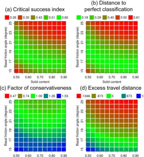
We now focus on the DII map and evaluate the perfor-mance of the deposition maps simulated with the various combinations of αs0 andδ against the ODA. Figure 11
il-lustrates the dependency of the model performance (defined by the parameters summarized in Table 4) on the combina-tion of αs0 andδ employed for a given model run. All four
parameters clearly indicate that, within the ranges tested, the
Figure 10.Results of Experiment 2A:(a)impact indicator index III and(b)deposition indicator index DII derived for the Acheron rock avalanche.
model results are sensitive to bothδandαs0.1L, CSI, and
D2PC display their optima nearδ=17◦as long asαs0≥0.7.
With higher fluid content, the optimum value ofδ increases, arriving at 20◦withαs0=0.5 (see Fig. 11a, b, and d). This
pattern appears plausible as far as a higher fluid content is supposed to increase the mobility of the flow, compensating for higher values ofδ. However, values ofαs0<0.7 are not
plausible at all for rock avalanches of this type. Forαs0≥0.7,
FoC displays its optimum of 1.0 atδ≥21◦, depending on αs0. FoC≈1.25 for the value ofδ where the other
parame-ters reach their optimum (see Fig. 11c). This would be fine for many applications in practice where slightly conservative results are desirable.
Consequently, we consider δ=17◦ and αs0=0.8 – in
addition to the parameter values given in Table 2 – one possible combination for back-calculating the Acheron rock avalanche. The simulation is repeated with exactly this com-bination (Experiment 2B). We note, however, that these pa-rameter values do not necessarily represent the real-world conditions, as the fluid content of rock avalanches may be much lower. Figure 12 shows the maps of HMax andHC,
both corresponding reasonably well to the OIA and the ODA, respectively. The slightly larger simulated than ob-served deposit (see Fig. 12b) corresponds to FoC≈1.25; the almost perfect correspondence of the observed and simu-lated termini corresponds to1L≈0. This means that the fact that the result is rather conservative than non-conservative (FoC>1) relates to lateral spreading rather than to the travel distance of the rock avalanche. Animation 2 in the Supple-ment illustrates the time evolution of the flow height in Ex-periment 2B.
4 Discussion
Figure 11.Validation and optimization of DII for the Acheron rock avalanche (see Table 4 for the criteria):(a)critical success index (CSI);(b) distance to perfect classification (D2PC);(c)factor of conservativeness (FoC);(d)excess travel distance (1L).
and the agreement of the observed and simulated deposition areas in Experiment 2B (see Sect. 3.2) appears reasonable. Yet, these experiments can neither replace model validation with observed process chains or interactions, nor can they re-place thorough multi-parameter sensitivity analysis and op-timization efforts, which will both be the subjects of future research. Fully documented two-phase process chains with readily available pre- and post-event DTMs are scarce. Pre-liminary r.avaflow results for the 2012 Santa Cruz multi-lake outburst flood in the Cordillera Blanca, Peru (Emmer et al., 2016), are however promising.
Experiment 2 serves for the demonstration of the pa-rameter sensitivity analysis and optimization functions of r.avaflow. The outcomes may be different when changing the cell size or any of the flow parameter values (see Ta-ble 2). Making r.avaflow fit for forward predictions will re-quire a thorough multi-parameter sensitivity analysis and op-timization campaign involving a large number and variety of well-documented events. Thereby, we aim at obtaining guid-ing parameter values – or, more appropriately, guidguid-ing pa-rameter ranges – for mass flow processes of different types and magnitudes. Approaches to perform such analyses are readily available, and some of them can be directly coupled to r.avaflow (Fischer, 2013; Fischer et al., 2015; Aaron et al., 2016; Krenn et al., 2016). However, due to the complex nature of two-phase mixture flows, r.avaflow depends on a relatively large number of flow parameters, a fact that
rep-Figure 12.Results of Experiment 2B.(a)Maximum flow height
HMax;(b)height of final depositHD(as entrainment is not
consid-ered,HD=HC). Note that, due to the predominance of solids, the
bluish and greenish colours indicated in the legend do not appear in the map (see Figs. 6–8).
resents a particular challenge in terms of the computational resources as well as in terms of visualization and interpreta-tion of the results of multi-parameter studies.
ex-pressed in topography-following coordinates are hardly com-patible with the data given in GIS coordinates.
A detailed and fully discrete description of the TVD-NOC scheme exists in the literature (Wang et al., 2004), and the scheme served well for various theoretical test cases (e.g. Pu-dasaini et al., 2014; Kafle et al., 2016; Kattel et al., 2016). However, we also identify two major drawbacks:
– Although the numerical scheme itself should be shock capturing and volume preserving (Tai et al., 2002; Wang et al., 2004), these properties may not fully hold in prac-tical applications (i.e. bounded gravitational mass flows with well-defined margins over complex topography). The complementary functions with ID 1–3 introduced in Sect. 2.4 partly compensate for the issues raised. – For real flow applications, full handling of the evolution
of the basal topography is not straightforward: the TVD-NOC scheme may introduce diffusion even though the evolution of the basal topography is not a standard trans-port equation. Entrainment is therefore, as a first step, included as a complementary function.
The numerical scheme employed will have to be enhanced to directly and effectively incorporate the complementary functions outlined in Sect. 2.4 in a fully consistent way. Ex-tensions of similar schemes have been tested for generic ex-amples (e.g. Zhai et al., 2015) and could serve as a valu-able basis also to implement a mechanical model for erosion, entrainment, and deposition (Pudasaini and Fischer, 2016). On the one hand, such an erosion model may build on ex-isting concepts (e.g. Fraccarollo and Capart, 2002; Sovilla et al., 2006; Medina et al., 2008; Armanini et al., 2009; Crosta et al., 2009; Hungr and McDougall, 2009; Le and Pitman, 2009; Iverson, 2012; Pirulli and Pastor, 2012). On the other hand, it may further require some fundamentally new ideas with regard to deposition.
5 Conclusions and outlook
We have introduced r.avaflow, a multifunctional open-source GIS application for simulating two-phase mass flows, pro-cess chains, and interactions. The outcomes of two compu-tational experiments have revealed that r.avaflow (i) has the capacity to simulate complex solid–fluid process interactions in a plausible way, and (ii) after the optimization of the basal friction angle and the solid content of the release mass, rea-sonably reproduces the observed deposition area of a doc-umented rock avalanche. However, it was out of the scope of the present work to validate the results obtained for com-plex process interactions against observed real-world data or even to conduct a comprehensive multi-parameter optimiza-tion campaign. Such efforts will be the next step towards making r.avaflow ready for the forward prediction of possible future mass flow events. Thereby, we will attempt to
estab-lish guiding parameter values for different types of processes and process magnitudes.
At the same time, we have identified a certain potential for the future enhancement of some the components of r.avaflow. The key challenges will consist in (i) integrating the model equations in an up-to-date numerical scheme, allowing to directly include the complementary functions, and (ii) re-placing the empirical entrainment model with a mechanical model for entrainment and deposition.
6 Code availability
The model codes along with a user manual are available at http://www.avaflow.org/software.html (Mergili et al., 2017).
7 Data availability
The scripts, the text file, and the GRASS locations with the spatial data required for reproducing the computational ex-periments described in Sect. 3 are available at http://www. avaflow.org/casestudies.html (Mergili and Krenn, 2017).
The Supplement related to this article is available online at doi:10.5194/gmd-10-553-2017-supplement.
Competing interests. The authors declare that they have no conflict of interest.
Acknowledgements. The work was conducted as part of the
international cooperation project “A GIS simulation model for avalanche and debris flows (avaflow)” supported by the German Research Foundation (DFG, project no. PU 386/3-1) and the Aus-trian Science Fund (FWF, project no. I 1600-N30). We are grateful to Matthias Benedikt and Matthias Rauter for comprehensive technical support.
Edited by: Simon Unterstrasser
Reviewed by: J. K. Kowalski and one anonymous referee
References
Armanini, A., Fraccarollo, L., and Rosatti, G.: Two-dimensional simulation of debris flows in erodible channels, Comput. Geosci., 35, 993–1006, 2009.
Berger, C., McArdell, B. W., and Schlunegger, F.: Sediment transfer patterns at the Illgraben catchment, Switzerland: Implications for the time scales of debris flow activities, Geomorphology, 125, 421–432, 2011.
Berger, M. J., George, D. L., LeVeque, R. J., and Mandli, K. T.: The GeoClaw software for depth-averaged flows with adaptive refinement, Adv. Water Res., 34, 1195–1206, 2011.
Chen, H., Crosta, G. B., and Lee, C. F.: Erosional effects on runout of fast landslides, debris flows and avalanches: A numerical in-vestigation, Geotechnique, 56, 305–322, 2006.
Christen, M., Bartelt, P., and Kowalski, J.: Back calculation of the In den Arelen avalanche with RAMMS: interpretation of model results, Ann. Glaciol., 51, 161–168, 2010a.
Christen, M., Kowalski, J., and Bartelt, B.: RAMMS: Numerical simulation of dense snow avalanches in three-dimensional ter-rain, Cold Reg. Sci. Technol., 63, 1–14, 2010b.
Courant, R., Friedrichs, K., and Lewy, H.: On the partial difference equations of mathematical physics, IBM J. Res. Dev., 11, 215– 234, 1967.
Crosta, G. B., Imposimato, S., and Roddeman, D.: Numerical mod-elling of entrainment/deposition in rock and debris-avalanches, Eng. Geol., 109, 135–145, 2009.
Davis, S. F.: Simplified second-order Godunov-type methods, SIAM J. Sci. Stat. Comp., 9, 445–473, 1988.
Denlinger, R. P. and Iverson, R. M.: Granular avalanches across irregular three-dimensional terrain: 1. Theory and computa-tion, J. Geophys. Res., 109, F01014, doi:10.1029/2003JF000085, 2004.
Emmer, A., Mergili, M., Juˇricová, A., Cochachin, A., and Huggel, C.: Insights from analyzing and modelling cascading multi-lake outburst flood events in the Santa Cruz Valley (Cordillera Blanca, Perú), EGU General Assembly, Vienna, Austria, 17–22 April 2016, EGU2016-2181, 2016.
Evans, S. G., Bishop, N. F., Fidel Smoll, L., Valderrama Murillo, P., Delaney, K. B., and Oliver-Smith, A: A re-examination of the mechanism and human impact of catastrophic mass flows orig-inating on Nevado Huascarán, Cordillera Blanca, Peru in 1962 and 1970, Eng. Geol., 108, 96–118, 2009.
Fischer, J.-T.: A novel approach to evaluate and compare computa-tional snow avalanche simulation, Nat. Hazards Earth Syst. Sci., 13, 1655–1667, doi:10.5194/nhess-13-1655-2013, 2013. Fischer, J.-T., Kowalski, J., and Pudasaini, S. P.: Topographic
curva-ture effects in applied avalanche modeling, Cold Reg. Sci. Tech-nol., 74, 21–30, 2012.
Fischer, J.-T., Kofler, A., Fellin, W., Granig, M., and Kleemayr, K.: Multivariate parameter optimization for computational snow avalanche simulation in 3d terrain, J. Glaciol., 61, 875–888, 2015.
Formetta, G., Capparelli, G., and Versace, P.: Evaluating perfor-mance of simplified physically based models for shallow land-slide susceptibility, Hydrol. Earth Syst. Sci., 20, 4585–4603, doi:10.5194/hess-20-4585-2016, 2016.
Fraccarollo, L. and Capart, H.: Riemann wave description of ero-sional dam-break flows, J. Fluid Mech., 461, 183–228, 2002. Gamma, P.: dfwalk – Ein Murgang-Simulationsprogramm zur
Gefahrenzonierung, Geographica Bernensia, G66, 144 pp., 2000.
GRASS Development Team: Geographic Resources Analysis Sup-port System (GRASS) Software, Version 7.0. Open Source Geospatial Foundation, 2015, available at: http://grass.osgeo.org, last access: 25 July 2016.
Grigoriyan, S. S., Eglit, M. E., and Yakimov, Y. L.: A new for-mulation and solution of the problem of the motion of a snow avalanche, Trudy Vycokogornogo Geofiziceskogo Instituta, 12, 104–113, 1967.
Guzzetti, F.: Landslide hazard and risk assessment, PhD disserta-tion, University of Bonn, Germany, Bonn, Germany, 2006. Hergarten, S. and Robl, J.: Modelling rapid mass movements using
the shallow water equations in Cartesian coordinates, Nat. Haz-ards Earth Syst. Sci., 15, 671–685, doi:10.5194/nhess-15-671-2015, 2015.
Horton, P., Jaboyedoff, M., Rudaz, B., and Zimmermann, M.: Flow-R, a model for susceptibility mapping of debris flows and other gravitational hazards at a regional scale, Nat. Hazards Earth Syst. Sci., 13, 869–885, doi:10.5194/nhess-13-869-2013, 2013. Huggel, C., Zgraggen-Oswald, S., Haeberli, W., Kääb, A., Polkvoj,
A., Galushkin, I., and Evans, S. G.: The 2002 rock/ice avalanche at Kolka/Karmadon, Russian Caucasus: assessment of extraordi-nary avalanche formation and mobility, and application of Quick-Bird satellite imagery, Nat. Hazards Earth Syst. Sci., 5, 173–187, doi:10.5194/nhess-5-173-2005, 2005.
Hungr, O.: A model for the runout analysis of rapid flow slides, de-bris flows, and avalanches, Can. Geotech. J., 32, 610–623, 1995. Hungr, O. and Evans, S. G.: Entrainment of debris in rock avalanches: an analysis of a long run-out mechanism, Geol. Soc. Am. Bull., 116, 1240–1252, 2004.
Hungr, O. and McDougall, S.: Two numerical models for landslide dynamic analysis, Comput. Geosci., 35, 978–992, 2009. Hungr, O., Corominas, J., and Eberhardt, E.: Estimating landslide
motion mechanism, travel distance and velocity, in: Landslide Risk Management, Proceedings, Vancouver Conference, Van-couver, Canada, 31 May–3 June 2005, State of the Art Paper #4, edited by: Hungr, O., Fell, R., Couture, R., and Eberhardt, E., Taylor and Francis Group, London, 99–128, 2005a.
Hungr, O., McDougall, S., and Bovis, M.: Entrainment of material by debris flows, in: Debris-flow hazards and related phenomena, edited by: Jakob, M. and Hungr, O., Springer, Berlin, Heidelberg, 135–158, 2005b.
Hutter, K. and Schneider L.: Important Aspects in the Formulation of Solid-Fluid Debris-Flow models. Part I: Thermodynamic Im-plications, Continuum Mech. Therm., 22, 363–390, 2010a. Hutter, K. and Schneider L.: Important Aspects in the Formulation
of Solid-Fluid Debris-Flow models. Part II: Constitutive Mod-elling, Continuum Mech. Therm., 22, 391–411, 2010b.
Iverson, R. M.: The physics of debris flows, Rev. Geophys., 35, 245–296, 1997.
Iverson, R. M.: Elementary theory of bed-sediment entrainment by debris flows and avalanches, J. Geophys. Res., 117, F03006, doi:10.1029/2011JF002189, 2012.
Iverson, R. M. and Denlinger, R. P.: Flow of variably fluidised gran-ular masses across three-dimensional terrain. I: Coulomb mixture theory, J. Geophys. Res., 106, 537–552, 2001.
Kafle, J., Pokhrel, P. R., Khattri, K. B., Kattel, P., Tuladhar, B. M., and Pudasaini, S. P.: Landslide-generated tsunami and particle transport in mountain lakes and reservoirs, Ann. Glaciol, 57, 232–244, 2016.
Kattel, P., Khattri, K. B., Pokhrel, P. R., Kafle, J., Tuladhar, B. M., and Pudasaini, S. P.: Simulating glacial lake outburst floods with a two-phase mass flow model, Ann. Glaciol., 57, 349–358, 2016. Kowalski, J. and McElwaine, J. N.: Shallow two-component gravity-driven flows with vertical variation, J. Fluid Mech., 714, 434–462, 2013.
Krenn, J., Mergili, M., Fischer, J.-T., Frattini, P., and Puda-saini, S. P.: Optimizing the parameterization of mass flow mod-els, in: Landslides and Engineered Slopes. Experience, Theory and Practice, edited by: Aversa, S., Cascini, L., Picarelli, L., and Scavia, C., Proceedings of the 12th International Symposium on Landslides, Napoli, Italy, CRC Press, Boca Raton, London, New York, Leiden, Chapter 135, 1195–1203, 2016.
Le, L. and Pitman, E. B.: A model for granular flows over an erodi-ble surface, SIAM J. Appl. Math., 70, 1407–1427, 2009. Lied, K. and Bakkehøi, S.: Empirical calculations of
snow-avalanche run-out distance based on topographic parameters, J. Glaciol., 26, 165–177, 1980.
Mangeney, A., Vilotte, J. P., Bristeau, M. O., Perthame, B., Bouchut, F., Simeoni, C., and Yerneni, S.: Numeri-cal modelling of avalanches based on Saint Venant equa-tions using a kinetic scheme, J. Geophys. Res., 108, 2527, doi:10.1029/2002JB002024, 2003.
Mangeney, A., Bouchut, F., Lajeunesse, E., Aubertin, A., Vilotte, J. P., and Pirulli, M.: On the use of Saint Venant equations to simulate the spreading of a granular mass, J. Geophys. Res., 110, B09103, doi:10.1029/2004JB003161, 2005.
McDougall, S. and Hungr, O.: A Model for the Analysis of Rapid Landslide Motion across Three-Dimensional Terrain, Can. Geotech. J., 41, 1084–1097, 2004.
McDougall, S. and Hungr, O.: Dynamic modeling of entrainment in rapid landslides, Can. Geotech. J., 42, 1437–1448, 2005. Medina, V., Hürlimann, M., and Bateman, A.: Application of
FLAT-Model, a 2D finite volume code, to debris flows in the northeast-ern part of the Iberian Peninsula, Landslides, 5, 127–142, 2008. Mergili, M. and Krenn, J.: r.avaflow – The open source GIS
simula-tion model for granular avalanches and debris flows. Case studies for computational experiments, available at: http://www.avaflow. org/casestudies.html, last access: 29 January 2017.
Mergili, M., Schratz, K., Ostermann, A., and Fellin, W.: Physically-based modelling of granular flows with Open Source GIS, Nat. Hazards Earth Syst. Sci., 12, 187–200, doi:10.5194/nhess-12-187-2012, 2012.
Mergili, M., Marchesini, I., Alvioli, M., Metz, M., Schneider-Muntau, B., Rossi, M., and Guzzetti, F.: A strategy for GIS-based 3-D slope stability modelling over large areas, Geosci. Model Dev., 7, 2969–2982, doi:10.5194/gmd-7-2969-2014, 2014. Mergili, M., Krenn, J., and Chu, H.-J.: r.randomwalk v1, a
multi-functional conceptual tool for mass movement routing, Geosci. Model Dev., 8, 4027–4043, doi:10.5194/gmd-8-4027-2015, 2015.
Mergili, M., Benedikt, M., and Pudasaini, S. P.: r.avaflow – The open source GIS simulation model for granular avalanches and debris flows, r.avaflow distributions, http://www.avaflow.org/ software.html, last access: 29 January 2017.
Nessyahu, H. and Tadmor, E.: Non-oscillatory central differencing for hyperbolic conservation laws, J. Comput. Phys., 87, 408–463, 1990.
Neteler, M. and Mitasova, H.: Open source GIS: a GRASS GIS ap-proach, Springer, New York, 2007.
Pastor, M., Haddard, B., Sorbino, G., Cuomo, S., and Drempetic, V.: A depth-integrated, coupled SPH model for flow-like landslides and related phenomena, Int. J. Numer. Anal. Met., 33, 143–172, 2009.
Pirulli, M. and Pastor, M.: Numerical study on the entrainment of bed material into rapid landslides, Geotechnique, 62, 959–972, 2012.
Pitman, E. B. and Le, L.: A two-fluid model for avalanche and de-bris flows, Philos. T. Roy. Soc. A,363, 1573–1601, 2005. Pitman, E. B., Nichita, C. C, Patra, A. K, Bauer, A. C., Bursik, M.,
and Weber, A.: A model of granular flows over an erodible sur-face, Discrete Cont. Dyn.-B., 3, 589–599, 2003a.
Pitman, E. B., Nichita, C. C., Patra, A. K., Bauer, A., Sheridan, M., and Bursik, M.: Computing granular avalanches and landslides, Phys. Fluids, 15, 3638–3646, 2003b.
Popinet, S.: An accurate adaptive solver for surface-tension-driven interfacial flows, J. Comput. Phys., 228, 5838–5866, 2009. Pudasaini, S. P.: A general two-phase debris flow model, J.
Geo-phys. Res., 117, F03010, doi:10.1029/2011JF002186, 2012. Pudasaini, S. P.: Dynamics of submarine debris flow and tsunami,
Acta Mech., 225, 2423–2434, doi:10.1007/s00707-014-1126-0, 2014.
Pudasaini, S. P. and Fischer, J.-T.: A mechanical erosion model for two-phase mass flows, arXiv:1610.01806, 2016.
Pudasaini, S. P. and Hutter, K.: Rapid shear flows of dry granular masses down curved and twisted channels, J. Fluid Mech., 495, 193–208, 2003.
Pudasaini, S. P. and Hutter, K.: Avalanche Dynamics: Dynamics of rapid flows of dense granular avalanches, Springer, Berlin, Hei-delberg, 2007.
Pudasaini, S. P. and Krautblatter, M.: A two-phase mechanical model for rock-ice avalanches, J. Geophys. R.-Earth, 119, 2272– 2290, 2014.
Pudasaini, S. P., Wang, Y., and Hutter, K.: Modelling debris flows down general channels, Nat. Hazards Earth Syst. Sci., 5, 799– 819, doi:10.5194/nhess-5-799-2005, 2005.
Pudasaini, S. P., Wang, Y., Sheng, L.-T., Hsiau, S.-S., Hutter, K., and Katzenbach, R.: Avalanching granular flows down curved and twisted channels: Theoretical and experimental results, Phys. Fluids, 20, 073302, doi:10.1063/1.2945304, 2008.
R Core Team: R: A Language and Environment for Statistical Com-puting, R Foundation for Statistical ComCom-puting, Vienna, Austria, available at: http://www.R-project.org, last access: 25 July 2016. Reid, M. E., Iverson, R. M., Logan, M., Lahusen, R. G., Godt, J. W., and Griswold, J. P.: Entrainment of bed sediment by debris flows: results from large-scale experiments, in: 5th International Con-ference on Debris-Flow Hazards “Mitigation, Mechanics, Pre-diction and Assessment”, 14–17 June 2011, Padua, Italy, edited by: Genevois, R., Hamilton, D. L., and Prestininzi, A., Italian Journal of Engineering Geology and Environment – Book, La Sapienza, Rome, 367–374, 2011.
by: Rickenmann, D. and and Chen, C.-L., Millpress, Rotterdam, 883–894. 2003.
Sampl, P. and Zwinger, T.: Avalanche Simulation with SAMOS, Ann. Glaciol., 38, 393–398, 2004.
Savage, S. B. and Hutter, K.: The motion of a finite mass of granular material down a rough incline, J. Fluid Mech., 199, 177–215, 1989.
Savage, S. B. and Iverson, R. M.: Surge dynamics coupled to pore-pressure evolution in debris flows, in: Debris-Flow Hazards Mit-igation: Mechanics, Prediction and Assessment, edited by: Rick-enmann, D. and Chen, C.-L., Millpress, Rotterdam, 503–514, 2003.
Smith, G. M., Davies, T. R., McSaveney, M. J., and Bell, D. H.: The Acheron rock avalanche, Canterbury, New Zealand – morphol-ogy and dynamics, Landslides, 3, 62–72, 2006.
Sovilla, B., Burlando, P., and Bartelt, P.: Field experiments and numerical modeling of mass entrainment in snow avalanches, J. Geophys. Res., 111, F03007, doi:10.1029/2005JF000391, 2006.
Tai, Y. C., Noelle, S., Gray, J. M. N. T., and Hutter, K.: Shock-capturing and front-tracking methods for granular avalanches, J. Comput. Phys., 175, 269–301, 2002.
Takahashi, T.: Debris Flow, IAHR Monograph Series, Balkema, The Netherlands, 1991.
Toro, E. F.: Riemann problems and the waf method for solving the twodimensional shallow water equations, Philos. T. Roy. Soc. A, 338, 43–68, 1992.
Van Westen, C. J., van Asch, T. W. J., and Soeters, R.: Landslide hazard and risk zonation: why is it still so difficult?, B. Eng. Geol. Environ., 65, 176–184, 2005.
Voellmy, A.: Über die Zerstörungskraft von Lawinen, Schweiz-erische Bauzeitung, 73, 159–162, 212–217, 246–249, 280–285, 1955.
Wang, Y., Hutter, K., and Pudasaini, S. P.: The Savage-Hutter the-ory: A system of partial differential equations for avalanche flows of snow, debris, and mud, J. Appl. Math. Mech., 84, 507–527, 2004.
Wichmann, V. and Becht, M.: Modeling of geomorphic processes in an alpine catchment, in: GeoDynamics: 7th International Con-ference on GeoComputation, Southampton, UK, 8–10 Septem-ber 2003, edited by: Atkinson, P. M, Foody, G. M., Darby, S. E., and Wu, F., 14 pp., 2003.