A comprehensive evaluation of multicategory classification methods for microbiomic data

R E S E A R C H

Open Access

A comprehensive evaluation of multicategory

classification methods for microbiomic data

Alexander Statnikov

, Mikael Henaff

, Varun Narendra

, Kranti Konganti

, Zhiguo Li

, Liying Yang

,

Zhiheng Pei

, Martin J Blaser

, Constantin F Aliferis

and Alexander V Alekseyenko

Abstract

Background:Recent advances in next-generation DNA sequencing enable rapid high-throughput quantitation of microbial community composition in human samples, opening up a new field of microbiomics. One of the promises of this field is linking abundances of microbial taxa to phenotypic and physiological states, which can inform development of new diagnostic, personalized medicine, and forensic modalities. Prior research has

demonstrated the feasibility of applying machine learning methods to perform body site and subject classification with microbiomic data. However, it is currently unknown which classifiers perform best among the many available alternatives for classification with microbiomic data.

Results:In this work, we performed a systematic comparison of 18 major classification methods, 5 feature selection methods, and 2 accuracy metrics using 8 datasets spanning 1,802 human samples and various classification tasks: body site and subject classification and diagnosis.

Conclusions:We found that random forests, support vector machines, kernel ridge regression, and Bayesian logistic regression with Laplace priors are the most effective machine learning techniques for performing accurate

classification from these microbiomic data.

Keywords:Microbiomic data, Machine learning, Classification, Feature selection

Background

Advances in low-cost, high-throughput DNA sequencing technologies have enabled the studies of the composition of microbial communities at unprecedented throughput levels. Such studies are particularly interesting for bio-medicine because for every human cell in the body there are about ten microbial cells in the gut alone [1]. These microbial symbionts contribute a meta-genome to human biology and interact with the human host to perform a multitude of functions ranging from basic metabolism to immune system development. Therefore, it is conceivable that the study of microbial compositions will yield important clues in understanding, diagnosing, and treating diseases by inferring the contribution of

each constituent of microbiota to various disease and physiological states.

A typical microbiomic study relies on a marker gene (or a group of markers) that can be used for the identifi-cation and quantitation of the microbes present in a given specimen. A good marker gene needs to have three essential properties: (i) it must be present in all of the microbes that we try to identify, (ii) its sequences should be conserved in members of the same species, and (iii) the interspecies difference in the gene sequence should be sufficiently significant to allow for taxonom-ical discrimination. The 16S rRNA gene is commonly used in microbiomic studies as a marker gene to gener-ate human microbiota surveys. For every sample in a dataset, a human microbiota survey contains hundreds of thousands or millions of DNA sequences from the underlying microbial community. Abundances of oper-ational taxonomic units (OTUs), extracted from the high-throughput sequencing data using upstream bio-informatic processing pipelines, can serve as input features for machine learning algorithms.

* Correspondence:[email protected];alexander. [email protected]

1

Center for Health Informatics and Bioinformatics, New York University Langone Medical Center, 227 East 30th Street, New York, NY, USA 2

Department of Medicine, New York University School of Medicine, 550 First Ave, New York, NY, USA

Full list of author information is available at the end of the article

A necessary prerequisite for the creation of successful microbiomics-based models is a solid understanding of the relative strengths and weaknesses of available machine learning and related statistical methods. Prior work by Knightset al. took an excellent first step in this direction and established the feasibility of creating accurate models for classification of body sites and subject identification [2]. The present work extends prior research by: (i) addressing diagnostic/personalized medicine applications in addition to classification of body sites and subjects, (ii) evaluating a large number of machine learning classification and feature/OTU selection methods, (iii) using more powerful multicategory classifiers based on a one-versus-rest scheme [3,4], (iv) measuring classification accuracy by a metric that is insensitive to prior distribution of classes, and (v) performing formal statistical comparison among classifiers. The present study thus allows determination of the classifiers that perform best for microbiomic data among the many available alternatives. It also allows identification of the best performing combinations of classification and feature/OTU selection algorithms across most microbiomic datasets.

We undertook a rigorous comparison of 18 major ma-chine learning methods for multicategory classification, 5 feature/OTU selection methods, and 2 accuracy met-rics using 8 datasets spanning 1,802 human samples and various classification tasks: body site and subject classifi-cation and diagnosis. We focused here on supervised classification methods because unsupervised methods (such as clustering and principal component analysis), which are designed to reveal structure of the data, pro-vide visual summaries, and help quality control, are not optimal (and depending on application may also be completely inadvisable) for predictively linking the data to specific response variables/phenotypes [5,6]. We found that random forests, support vector machines, kernel ridge regression, and Bayesian logistic regression with Laplace priors are the most effective machine learning techniques in performing accurate classification from microbiomic data.

Methods

Datasets and data preparatory steps

In this work, we used eight microbiomic datasets (Table 1). All datasets were 16S rRNA gene surveys obtained with 454 pyrosequencing. The datasets CBH, CS, CSS, FS, FSH were obtained from the study of Knights et al. [2] and originate from the works of Costello et al. [7] [SRA: ERP000071] and Fierer et al. [8] [SRA: SRA0102034.1]. The dataset BP was obtained from the laboratory of Martin J. Blaser (Alekseyenko AV, Perez-Perez GI, D’Souza A, Strober B, Gao Z, Methe B, Blaser MJ: Population differen-tiation of the cutaneous microbiota in psoriasis, forthcom-ing), [9] and the datasets PBS and PDX were obtained from

the laboratory of Zhiheng Pei [10] at New York University (NYU) Langone Medical Center.

A major data preparatory step in the analysis of human microbiota gene surveys is the extraction of operational taxonomic units (OTUs) that serve as input features for machine learning algorithms. An OTU is a cluster of sequences of non-human origin that is constructed based on nucleotide similarity between the sequences. The necessity to use sequence similarity-based OTUs is motivated by two major considerations: (i) good reference databases may not be available for fine-grained taxo-nomic classification of sequences, and (ii) sequencing errors introduced by the technologies are effectively controlled when sequences are aggregated into similarity-based clusters.

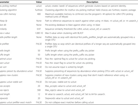
The OTUs were constructed using UCLUST software version 1.2.22q (http://www.drive5.com/usearch/, [11]) at a sequence similarity threshold of 97%, as recommended in the study [2]. UCLUST was applied after processing the raw DNA sequencing data with the Quantitative Insights Into Microbial Ecology (QIIME) pipeline version 1.3.0 (http://qiime.org/), which is specifically designed for high-throughput 16S rRNA sequencing studies [12]. All param-eter values used for processing are provided in Table 2.

In summary, we started with raw DNA sequencing data, removed human DNA sequences, defined OTUs over microbial sequences, and quantified relative abun-dance of all sequences that belong to each OTU. These relative abundances, further rescaled to the range [0, 1], served as input features for machine learning algorithms. The number of OTUs in each dataset is provided in Table 1. We emphasize that the OTUs were constructed without knowledge of classification labels and thus do not bias performance of machine learning techniques.

The OTU tables and sample labels for all datasets used in the study are provided in Additional files 1, 2, 3, 4, 5, 6, 7 and 8.

Machine learning algorithms for classification

Table 2 Values of parameters of the preprocessing methods [2,11,12]

Parameter Value Description

otu picking method uclust uclust, creates‘seeds’of sequences which generate clusters based on percent identity.

clustering algorithm furthest Clustering algorithm for mothur otu picking method. Valid choices are: furthest, nearest, average.

max cdhit memory 400 Maximum available memory to cd-hit-est (via the program’s -M option) for cdhit OTU picking method (units of Mbyte)

refseqs fp None Path to reference sequences to search against when using -m blast, -m uclust_ref, or -m usearch_ref

blast db None Pre-existing database to blast against when using -m blast

similarity 0.97 Sequence similarity threshold (for cdhit, uclust, uclust_ref, or usearch)

max e value 1.00E-10 Max E-value when clustering with BLAST

prefix prefilter length None Prefilter data so seqs with identical first prefix_prefilter_length are automatically grouped into a single OTU

trie prefilter FALSE Prefilter data so seqs which are identical prefixes of a longer seq are automatically grouped into a single OTU

prefix length 50 Prefix length when using the prefix_suffix otu picker

suffix length 50 Suffix length when using the prefix_suffix otu picker

optimal uclust FALSE Pass the -optimal flag to uclust for uclust otu picking.

exact uclust FALSE Pass the -exact flag to uclust for uclust otu picking.

user sort FALSE Do not assume input is sorted by length

suppress presort by abundance uclust FALSE Suppress presorting of sequences by abundance when picking OTUs with uclust or uclust_ref

suppress new clusters FALSE Suppress creation of new clusters using seqs that don_’t match reference when using -m uclust_ref or -m usearch_ref

suppress uclust stable sort FALSE Do not pass -stable-sort to uclust

max accepts 20 Max_accepts value to uclust and uclust_ref

max rejects 500 Max_rejects value to uclust and uclust_ref

word length 12 W value to usearch, uclust, and uclust_ref. Set to 64 for usearch.

stepwords 20 Stepwords value to uclust and uclust_ref

suppress uclust prefilter exact match FALSE Do not collapse exact matches before calling uclust Table 1 Characteristics of microbiomic datasets used in this study

Dataset Number

of samples

Number of features (OTUs)

Number of classes

Classification task and samples per class Max. prior probability of a class (%)

Costello Body Habitat (CBH) 552 6,979 6 Classify body habitats: Skin (357), Oral Cavity (46), External Auditory Canal (44), Hair (14), Nostril (46), Feces (45)

64.7

Costello Subject (CS) 140 2,543 7 Classify 7 subjects by microbiota (20/20/20/20/20/20/20) 14.3

Costello Skin Sites (CSS) 357 4,793 12 Classify skin sites: external nose (14), forehead (32), glans penis (8), labia minora (6), axilla (28), pinna (27), palm (64), palmar index finger (28), plantar foot (64), popliteal fossa (46), volar forearm (28), umbilicus (12)

17.9

Fierer Subject (FS) 104 1,217 3 Classify 3 subjects by microbiota (40/33/31) 38.5

Fierer Subject x Hand (FSH) 98 1,217 6 Classify by subject and left/right hand (20/18/17/14/16/13)

20.4

Blaser Psoriasis (BP) 151 13,503 3 Classify as Control (49), Psoriasis Normal (51), Psoriasis Lesion (51)

33.8

Pei Diagnosis (PDX) 200 74,018 4 Classify as Normal (28), Reflux Esophagitis (36), Barrett's Esophagus (84), Esophageal Adenocarcinoma (52)

42.0

Pei Body Site (PBS) 200 74,018 4 Classify body site: Oral Cavity (51), Esophagus (51), Stomach (48), Stool (50)

for each class against the rest and then classified new sam-ples by taking a vote of the binary classifiers and choosing the class with the ‘strongest’ vote. The one-versus-rest approach for classification is known to be among the best performing methods for multicategory classification for other types of data, including microarray gene expression [3,4]. Random forests, k-nearest neighbors, and probabil-istic neural networks methods can solve multicategory problems natively and were applied directly.

Support vector machines (SVMs) are a class of machine learning algorithms that perform classification by separat-ing the different classes in the data usseparat-ing a maximal margin hyperplane [13]. To learn non-linear decision boundaries, SVMs implicitly map the data to a higher dimensional space by means of a kernel function, where a separating hyperplane is then sought. The superior empirical per-formance of SVMs in many types of high-throughput biomedical data can be explained by several theoretical reasons: for example, SVMs are robust to high variable-to-sample ratios and large numbers of features, they can efficiently learn complex classification functions, and they employ powerful regularization principles to avoid overfitting [3,14]. Extensive literature on applications in text categorization, image recognition and other fields also show the excellent empirical performance of this classifier in many other domains. SVMs were used with linear kernel, polynomial kernel, and a radial basis function (RBF, also known as Gaussian) kernel.

Kernel ridge regression (KRR) adds the kernel trick to ridge regression. Ridge regression is linear regression with regularization by an L2penalty. Kernel ridge regres-sion and SVMs are similar in dealing with non-linearity (by using the kernel trick) and model regularization (by using an L2penalty, also called the ridge). The differ-ence lies in the loss function: the SVMs use a hinge loss function, while ridge regression uses squared loss [15].

Regularized Logistic Regressionadds regularization by an L1or L2penalty to the logistic regression (abbreviated as L1-LR and L2-LR, respectively) [16,17]. Logistic regression is a learning method from the class of general linear models that learns a set of weights that can be used to predict the probability that a sample belongs to a given class [18]. The weights are learned by minimizing a log-likelihood loss function. The model is regularized by impos-ing an L1or L2penalty on the weight vector. An L2penalty favors solutions with relatively small coefficients, but does not discard any features. An L1penalty shrinks the weights more uniformly and can set weights to zero, effectively performing embedded feature selection.

Bayesian logistic regression (BLR) is another method from the class of general linear models that finds the maximum a posteriori estimate of the weight vector under either Gaussian or Laplace prior distributions, using a coordinate descent algorithm [19,20]. Gaussian

priors tend to favor dense weight vectors, whereas Laplace priors lead to sparser solutions; in this way they perform a similar purpose as imposing an L1penalty on the coefficients.

Random forests (RF) is a classification algorithm that uses an ensemble of unpruned decision trees, each built on a bootstrap sample of the training data using a randomly selected subset of features [21]. The random forest algorithm possesses a number of appealing proper-ties, making it well-suited for classification of microbiomic data: (i) it is applicable when there are more predictors than observations; (ii) it performs embedded feature selection and it is relatively insensitive to the large number of irrelevant features; (iii) it incorporates interactions be-tween predictors: (iv) it is based on the theory of ensemble learning that allows the algorithm to learn accurately both simple and complex classification functions; (v) it is applic-able for both binary and multicategory classification tasks; and (vi) according to its inventors, it does not require much fine tuning of parameters and the default parameterization often leads to excellent classification accuracy [21].

K-nearest neighbors (KNN) algorithm treats all objects as points inm-dimensional space (wheremis the number of features) and given an unseen object, the algorithm classifies it by a vote of K nearest training objects as determined by some distance metric, typically Euclidian distance [15,22].

Probabilistic Neural Networks (PNN) belong to the family of Radial Basis Function (RBF) neural networks [22], and are composed of an input layer, a hidden layer consisting of a pattern layer and a competitive layer, and an output layer (see [23,24]). The pattern layer contains one unit for each object in the training dataset. Given an unseen training object, each unit in the pattern layer computes a distance from this object to objects in the training set and applies a Gaussian density activation function. The competitive layer contains one unit for each classification category, and these units receive input only from pattern units that are associated with the classification category to which the training object belongs. Each unit in the competitive layer sums over the outputs of the pattern layer and computes a probability of the object belonging to a specific classification category. Finally, the output unit corresponding to the maximum of these probabilities outputs ‘1’, while those remaining output‘0’.

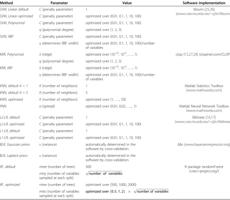
Table 3 describes software implementations for each classifier.

Parameters of machine learning classification algorithms

For SVMs and KRR, we used the following polynomial kernel:

K xð ;yÞ ¼xTyþ1q and RBF kernel:

K xð ;yÞ ¼ expγkxyk2;

where x and y are samples with sequence abundances and q and γ are kernel parameters. Table 3 describes the parameter values for each classifier.

Model/parameter selection and accuracy estimation strategy

For model/parameter selection and accuracy estimation, we used nested repeated 10-fold cross-validation [29,30].

The inner loop of cross-validation was used to determine the best parameters of the classifier (that is, values of parameters yielding the best accuracy for the validation dataset). The outer loop of cross-validation was used for estimating the accuracy of the classifier that was built using the previously found best parameters by testing with an independent set of samples. To account for variance in accuracy estimation, we repeated this entire process (nested 10-fold cross-validation) for 10 different splits of the data into 10 cross-validation testing sets and averaged the results [29].

Feature/operational taxonomic unit (OTU) selection methods

We used the following feature selection techniques in an effort to improve classification accuracy, alleviate the ‘curse of dimensionality’and improve interpretability by Table 3 Parameters and software implementations of the classification algorithms

Method Parameter Value Software implementation

SVM, Linear default C(penalty parameter) 1 libsvm [25,26]

(www.csie.ntu.edu.tw/~cjlin/libsvm/) SVM, Linear optimized C(penalty parameter) optimized over (0.01, 0.1, 1, 10, 100)

SVM, Polynomial C(penalty parameter) optimized over (0.01, 0.1, 1, 10, 100)

q(polynomial degree) optimized over (1, 2, 3)

SVM, RBF C(penalty parameter) optimized over (0.01, 0.1, 1, 10, 100)

γ(determines RBF width) optimized over (0.01, 0.1, 1, 10, 100)/number of variables

KRR, Polynomial λ(ridge) optimized over (10-10_{, 10}-9_{,. . ., 1) clop [15,27,28] (clopinet.com/CLOP/)}

q(polynomial degree) optimized over (1, 2, 3)

KRR, RBF λ(ridge) optimized over (10-10_{, 10}-9_{,. . ., 1)}

γ(determines RBF width) optimized over (0.01, 0.1, 1, 10, 100)/number of variables

KNN, default K = 1 K(number of neighbors) 1 Matlab Statistics Toolbox

(www.mathworks.com) KNN, default K = 5 K(number of neighbors) 5

KNN, optimized K(number of neighbors) optimized over (1,. . ., 50)

PNN σ(spread) optimized over (0.01, 0.02,. . ., 1) Matlab Neural Network Toolbox (www.mathworks.com)

L2-LR, default C(penalty parameter) 1 liblinear [16,17]

(www.csie.ntu.edu.tw/~cjlin/liblinear/) L2-LR, optimized C(penalty parameter) optimized over (0.01, 0.1, 1, 10, 100)

L1-LR, default C(penalty parameter) 1

L1-LR, optimized C(penalty parameter) optimized over (0.01, 0.1, 1, 10, 100)

BLR, Gaussian priors v(variance) automatically determined in the software by cross-validation

bbr (www.bayesianregression.org)

BLR, Laplace priors v(variance) automatically determined in the software by cross-validation

RF, default ntree(number of trees) 500 R package randomForest

(cran.r-project.org/) mtry(number of variables

sampled at each split)

ffiffiffiffiffiffiffiffiffiffiffiffiffiffiffiffiffiffiffiffiffiffiffiffiffiffiffiffiffiffiffiffiffiffiffiffiffiffiffiffiffiffi

number of variables p

RF, optimized ntree(number of trees) optimized over (500, 1000, 2000)

mtry(number of variables

sampled at each split) optimized over

0:5;1;2

determining which OTUs were predictive of the different responses:

Random forest-based backward elimination procedure RFVS [31]: We applied thevarSelRFimplementation of the RFVS method (http://cran.r-project.org/web/ packages/varSelRF) with the recommended

parameters:ntree= 2000,mtryFactor= 1,nodesize=

1,fraction.dropped= 0.2 (a parameter denoting

fraction of OTUs with low importance values to be discarded during the backward elimination procedure), andc.sd= 0 (a factor that multiplies the standard deviation of error for stopping iterations and choosing the best performing subset of OTUs). We refer to this method as‘RFVS1.’

The RFVS procedure as described above, except that

c.sd= 1 (denoted as‘RFVS2’): This method differs from RFVS1 in that it performs statistical

comparison to return the smallest subset of OTUs with classification accuracy that is not statistically distinguishable from the nominally best one. The SVM-based recursive feature elimination

method SVM-RFE [32]: To be comparable with the RFVS method, we used the fraction of OTUs that are discarded in the iterative SVM models equal to 0.2. This variable selection method was optimized separately for the employed accuracy metrics. We used implementation of SVM-RFE on top of the libSVM library [25,26].

A backward elimination procedure based on univariate ranking of OTUs with Kruskal-Wallis one-way non-parametric ANOVA [3] (denoted as ‘KW’): Similarly to SVM-RFE and RFVS, we performed backward elimination by discarding 20% of the OTUs at each iteration. This variable selection method was optimized separately for the employed accuracy metrics. We used

implementation of this variable selection procedure on top of the libSVM library [25,26] and Matlab Statistics Toolbox.

We emphasize that all feature selection methods were applied during cross-validation utilizing only the training data and splitting it into smaller training and validation sets, as necessary. This ensures integrity of the model accuracy estimation by protecting against overfitting.

Accuracy metrics

We used two classification accuracy metrics: the proportion of correct classifications (PCC) and relative classifier infor-mation (RCI). The first is easy to interpret and simplifies statistical testing, but is sensitive to the prior class probabil-ities and does not fully describe the actual difficulty of the classification problem. For example, in the CBH dataset

where 357 out of 552 samples are drawn from the skin, a trivial classifier that would always predict the class of maximum prior probability would still obtain PCC = 0.647. On the other hand, a trivial classifier would achieve only PCC = 1/7 = 0.143 in the CS dataset where there are 20 samples from each of the 7 individuals that we want to classify.

The RCI metric is an entropy-based measure that quantifies how much the uncertainty of the decision problem is reduced by the classifier, relative to classifying by simply using the prior probabilities of each class [33]. As such, it corrects for differences in prior probabilities of the diagnostic categories, as well as the number of categories.

The values of both metrics range from 0 to 1, where 0 indicates worst and 1 indicates best classifi-cation performance.

Statistical comparison among classifiers

To test whether the differences in accuracy between the nominally best method (that is, the one with the highest average accuracy) and all remaining algorithms are non-random, we need a statistical comparison of the observed differences in accuracies. We used random permutation testing, as described in [34]. For every algorithmX, other than the nominally best algorithm Y, we performed the following steps: (I) we defined the null hypothesis (H0) to be algorithmXis as good asY, that is, the accuracy of the best algorithmYminus the accuracy of algorithmXis zero; (II) we obtained the permutation distribution ofΔXY, the es-timator of the true unknown difference between accuracies of the two algorithms under the null hypothesis, by repeat-edly swapping the accuracy measures ofXandYat random for each of the datasets and cross-validation testing sets; (III) we computed the cumulative probability (P value) of

ΔXYbeing greater than or equal to the observed difference

^

ΔXY over 10,000 permutations. This process was repeated for each of the 10 data splits, and the P values were averaged. If the resultingPvalue was smaller than 0.05, we rejected H0and concluded that the data support that algorithmXis not as good asYin terms of classification accuracy, and this difference is not due to sampling error. The procedure was run separately for PCC and RCI accuracy metrics.

Results and Discussion

Classification without feature/operational taxonomic unit (OTU) selection

datasets, and thePvalue associated with its statistical com-parison against the nominally best performing classifier.

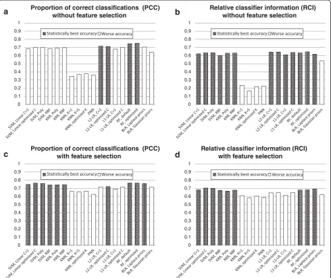
Notably, we obtain different results depending on which performance metric we use. In both cases, random for-ests with optimized parameters is the nominally best performing classifier. When using PCC as a performance metric, the nominally best performing classifier is statisti-cally significantly better than all other classifiers except for L2-regularized logistic regression and random forests with default parameters. However, when using RCI as a per-formance metric, the only classifiers which are statistically significantly worse than the nominally best performing classifier are the KNN-based methods, PNN and BLR with

Gaussian priors. Therefore, several classifiers which are significantly worse when using the somewhat naive PCC metric are comparable when using the more descriptive RCI metric (Figure 1a,b).

Classification with feature/operational taxonomic unit (OTU) selection

Classification accuracy results of experiments with feature/ OTU selection, averaged over 8 datasets, are provided in Figure 1c,d. Detailed dataset-by-dataset classification accur-acy results are shown in Tables 6 and 7. The tables present results for the best performing feature selection method for each classifier/dataset combination under the operating 0

0.1 0.2 0.3 0.4 0.5 0.6 0.7 0.8 0.9 1

Proportion of correct classifications (PCC) with feature selection

0 0.1 0.2 0.3 0.4 0.5 0.6 0.7 0.8 0.9 1

Proportion of correct classifications (PCC) without feature selection

0 0.1 0.2 0.3 0.4 0.5 0.6 0.7 0.8 0.9 1

Relative classifier information (RCI) without feature selection

0 0.1 0.2 0.3 0.4 0.5 0.6 0.7 0.8 0.9 1

Relative classifier information (RCI) with feature selection

a

c

b

d

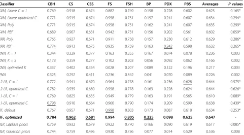
Table 4 Classification accuracy without feature/operational taxonomic unit (OTU) selection, measured by proportion of correct classifications (PCC)

Classifier CBH CS CSS FS FSH BP PDX PBS Averages Pvalues

SVM, Linear C = 1 0.920 0.911 0.583 0.940 0.598 0.354 0.468 0.695 0.684 0.022

SVM, Linear optimized C 0.920 0.911 0.622 0.980 0.585 0.383 0.485 0.709 0.699 0.038

SVM, Poly 0.920 0.911 0.622 0.980 0.585 0.383 0.484 0.709 0.699 0.036

SVM, RBF 0.909 0.904 0.575 0.973 0.575 0.379 0.451 0.700 0.683 0.021

KRR, Poly 0.913 0.918 0.581 0.954 0.598 0.377 0.482 0.709 0.692 0.027

KRR, RBF 0.923 0.904 0.618 0.967 0.632 0.366 0.467 0.709 0.698 0.030

KNN, K = 1 0.496 0.360 0.195 0.451 0.305 0.249 0.419 0.291 0.346 0.002

KNN, K = 5 0.713 0.339 0.188 0.397 0.281 0.331 0.393 0.300 0.368 0.001

KNN, optimized K 0.714 0.377 0.192 0.325 0.273 0.340 0.409 0.379 0.376 0.001

PNN 0.743 0.321 0.216 0.522 0.332 0.325 0.167 0.247 0.359 0.000

L2-LR, C = 1 0.934 0.939 0.628 0.982 0.628 0.380 0.515 0.725 0.716 0.084*

L2-LR, optimized C 0.933 0.938 0.623 0.978 0.618 0.383 0.502 0.725 0.712 0.067*

L1-LR, C = 1 0.929 0.801 0.559 0.975 0.700 0.422 0.384 0.673 0.680 0.018*

L1-LR, optimized C 0.928 0.903 0.561 0.981 0.690 0.445 0.412 0.692 0.702 0.039

RF, default 0.932 0.955 0.673 0.999 0.744 0.508 0.424 0.730 0.746 0.270*

RF, optimized 0.938 0.956 0.689 0.994 0.760 0.523 0.423 0.735 0.752

-BLR, Laplace priors 0.927 0.927 0.634 0.962 0.622 0.387 0.452 0.727 0.705 0.042

BLR, Gaussian priors 0.921 0.736 0.480 0.966 0.631 0.354 0.410 0.635 0.642 0.008

The nominally best performing classifier on average over all datasets is marked with bold, andPvalues of methods whose performance cannot be deemed statistically worse than the nominally best performing method are marked with“*”. The accuracy of the nominally best performing method for each dataset is underlined.

Table 5 Classification accuracy without feature/operational taxonomic unit (OTU) selection, measured by relative classifier information (RCI)

Classifier CBH CS CSS FS FSH BP PDX PBS Averages Pvalues

SVM, Linear C = 1 0.769 0.918 0.674 0.882 0.749 0.158 0.228 0.602 0.623 0.165*

SVM, Linear optimized C 0.771 0.915 0.674 0.958 0.751 0.157 0.241 0.607 0.634 0.294*

SVM, Poly 0.771 0.915 0.674 0.958 0.751 0.162 0.241 0.607 0.635 0.299*

SVM, RBF 0.689 0.907 0.631 0.942 0.731 0.156 0.202 0.561 0.602 0.059*

KRR, Poly 0.765 0.927 0.671 0.911 0.758 0.157 0.230 0.612 0.629 0.206*

KRR, RBF 0.774 0.913 0.675 0.935 0.759 0.163 0.242 0.598 0.632 0.265*

KNN, K = 1 0.344 0.329 0.377 0.163 0.355 0.167 0.074 0.078 0.236 0.003

KNN, K = 5 0.178 0.359 0.277 0.102 0.203 0.056 0.092 0.062 0.166 0.002

KNN, optimized K 0.337 0.402 0.354 0.028 0.207 0.089 0.122 0.196 0.217 0.003

PNN 0.325 0.292 0.411 0.236 0.342 0.041 0.070 0.089 0.226 0.002

L2-LR, C = 1 0.772 0.941 0.670 0.964 0.778 0.161 0.236 0.628 0.644 0.575*

L2-LR, optimized C 0.782 0.939 0.680 0.958 0.778 0.163 0.228 0.624 0.644 0.626*

L1-LR, C = 1 0.769 0.825 0.635 0.949 0.779 0.163 0.191 0.565 0.610 0.089*

L1-LR, optimized C 0.798 0.910 0.664 0.960 0.790 0.174 0.209 0.599 0.638 0.439*

RF, default 0.767 0.957 0.671 0.998 0.803 0.173 0.087 0.618 0.634 0.253*

RF, optimized 0.784 0.962 0.681 0.994 0.805 0.225 0.098 0.625 0.647

-BLR, Laplace priors 0.759 0.932 0.679 0.922 0.770 0.166 0.090 0.619 0.617 0.085*

BLR, Gaussian priors 0.744 0.759 0.496 0.930 0.736 0.077 0.014 0.529 0.536 0.008

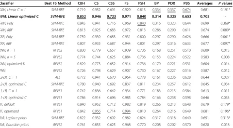
Table 6 Classification accuracy with feature/operational taxonomic unit (OTU) selection, measured by proportion of correct classifications (PCC)

Classifier Best FS Method CBH CS CSS FS FSH BP PDX PBS Averages Pvalues

SVM, Linear C = 1 SVM-RFE 0.900 0.941 0.610 0.965 0.719 0.524 0.558 0.759 0.747 0.319*

SVM, Linear optimized C SVM-RFE 0.952 0.935 0.631 0.985 0.754 0.534 0.553 0.761 0.763 0.535*

SVM, Poly SVM-RFE 0.950 0.929 0.633 0.987 0.742 0.528 0.551 0.754 0.759 0.460*

SVM, RBF SVM-RFE 0.941 0.918 0.617 0.987 0.693 0.518 0.523 0.727 0.741 0.179*

KRR, Poly KW 0.909 0.933 0.623 0.949 0.749 0.547 0.514 0.713 0.742 0.199*

KRR, RBF KW 0.929 0.939 0.634 0.970 0.737 0.537 0.504 0.714 0.745 0.248*

KNN, K = 1 RFVS2 0.930 0.760 0.563 0.971 0.623 0.421 0.443 0.596 0.663 0.011

KNN, K = 5 RFVS2 0.930 0.724 0.529 0.943 0.656 0.434 0.434 0.609 0.657 0.009

KNN, optimized K RFVS2 0.935 0.754 0.552 0.963 0.648 0.422 0.432 0.620 0.666 0.011

PNN RFVS2 0.906 0.781 0.560 0.956 0.623 0.130 0.449 0.604 0.626 0.006

L2-LR, C = 1 ALL 0.934 0.939 0.628 0.982 0.628 0.380 0.515 0.725 0.716 0.047

L2-LR, optimized C KW 0.921 0.948 0.650 0.836 0.739 0.499 0.464 0.711 0.721 0.089*

L1-LR, C = 1 RFVS1 0.922 0.818 0.589 0.968 0.706 0.449 0.395 0.687 0.692 0.020

L1-LR, optimized C RFVS1 0.934 0.909 0.611 0.993 0.710 0.442 0.418 0.697 0.714 0.048

RF, default RFVS1 0.954 0.950 0.704 0.991 0.745 0.550 0.479 0.746 0.765

-RF, optimized RFVS1 0.954 0.950 0.695 0.996 0.746 0.548 0.479 0.741 0.764 0.498*

BLR, Laplace priors SVM-RFE 0.946 0.929 0.639 0.991 0.759 0.521 0.537 0.739 0.758 0.465*

BLR, Gaussian priors KW 0.926 0.856 0.557 0.980 0.728 0.525 0.426 0.701 0.713 0.043

The nominally best performing classifier on average over all datasets is marked with bold, andPvalues of methods whose performance cannot be deemed statistically worse than the nominally best performing method are marked with“*”. The accuracy of the nominally best performing method for each dataset is underlined.

Table 7 Classification accuracy with feature/ operational taxonomic unit (OTU) selection, measured by relative classifier information (RCI)

Classifier Best FS Method CBH CS CSS FS FSH BP PDX PBS Averages Pvalues

SVM, Linear C = 1 SVM-RFE 0.719 0.952 0.691 0.929 0.813 0.334 0.337 0.674 0.681 0.191*

SVM, Linear optimized C SVM-RFE 0.852 0.946 0.723 0.971 0.840 0.314 0.325 0.653 0.703

-SVM, Poly SVM-RFE 0.845 0.941 0.716 0.969 0.840 0.316 0.323 0.644 0.699 0.369*

SVM, RBF SVM-RFE 0.813 0.925 0.683 0.972 0.813 0.286 0.290 0.611 0.674 0.089*

KRR, Poly SVM-RFE 0.759 0.939 0.683 0.931 0.800 0.297 0.290 0.626 0.666 0.061*

KRR, RBF SVM-RFE 0.807 0.935 0.687 0.944 0.801 0.297 0.316 0.633 0.677 0.097*

KNN, K = 1 RFVS2 0.830 0.779 0.657 0.939 0.736 0.168 0.251 0.510 0.609 0.015

KNN, K = 5 RFVS2 0.774 0.744 0.625 0.884 0.736 0.153 0.224 0.522 0.583 0.008

KNN, optimized K RFVS2 0.829 0.773 0.652 0.914 0.736 0.179 0.221 0.531 0.604 0.014

PNN RFVS2 0.726 0.798 0.629 0.907 0.730 0.167 0.227 0.516 0.587 0.012

L2-LR, C = 1 ALL 0.772 0.941 0.670 0.964 0.778 0.161 0.236 0.628 0.644 0.027

L2-LR, optimized C SVM-RFE 0.780 0.940 0.692 0.837 0.811 0.234 0.257 0.612 0.645 0.034

L1-LR, C = 1 RFVS1 0.742 0.836 0.642 0.934 0.771 0.183 0.213 0.584 0.613 0.011

L1-LR, optimized C RFVS1 0.786 0.914 0.696 0.985 0.784 0.166 0.238 0.598 0.646 0.033

RF, default RFVS1 0.840 0.952 0.712 0.982 0.819 0.266 0.213 0.648 0.679 0.179*

RF, optimized RFVS1 0.842 0.956 0.714 0.994 0.810 0.264 0.216 0.649 0.681 0.196*

BLR, Laplace priors SVM-RFE 0.822 0.932 0.692 0.982 0.824 0.317 0.318 0.640 0.691 0.313*

BLR, Gaussian priors RFVS2 0.761 0.855 0.625 0.968 0.770 0.208 0.202 0.570 0.620 0.018

assumption that practitioners will optimize the choice of feature selection method for each dataset separately (using cross-validation or other suitable protocols). As before, for each classifier and feature selection method we include the performance on each individual dataset, the average performance over all datasets, and thePvalue associated with the statistical comparison test against the nominally best performing classifier.

For many methods, there is a significant improvement using feature/OTU selection prior to performing classifi-cation. For both accuracy metrics, there is no statistically significant difference between the performance of SVMs, kernel ridge regression and random forests. The improve-ment in performance due to feature selection is especially pronounced in the case of KNN and PNN, which is consistent with the general understanding that these methods are sensitive to a large number of irrelevant features. However, KNN and PNN are still among the worst performing classifiers (Figure 1c,d).

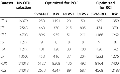
The number of OTUs selected on average across the 10 data splits and 10 cross-validation training sets is provided in Table 8. We note that feature/OTU selection was optimized for each accuracy metric separately to the extent that the feature selection methods allowed it. Specifically, we used the same accuracy metric for evaluating model accuracy internally in the SVM-RFE and KW feature selection methods as for evaluating the final classification accuracy on the testing sets. In the case of RFVS, we used the package provided by the authors which only allows the use of PCC for evalu-ation of model accuracy for the different subsets of variables [31]; hence, the same sets of features were used in both the PCC and RCI benchmarks. Finally, we note that in the present work we focus exclusively on classification accuracy and do not incorporate the number of selected OTUs in the comparison metrics

because there is no well-defined trade-off between the number of selected OTUs and the classification accuracy in the datasets studied.

Conclusions

In this work, we conducted a thorough evaluation to identify the most accurate machine learning algorithms for multicategory classification from microbiomic data. We evaluated 18 algorithms for multicategory classification, 5 feature selection methods and 2 accuracy metrics on 8 different classification tasks with human microbiomic data. We found that for the most part, SVMs, random forests, kernel ridge regression, and Bayesian logistic regression with Laplace priors provided statistically similar levels of classification accuracy. On the other hand, we also found that K-nearest neighbors and probabilistic neural networks were significantly outperformed by the other techniques.

The results of this work also highlight the large vari-ation in difficulty across the different classificvari-ation tasks. Tasks that involve classifying body sites, body habitats or subjects yield much higher accuracy rates than those which involve predicting the correct diagnosis, which are arguably more useful for real-life clinical applications. However, considering that the use of microbiomics for disease diagnosis has so far been relatively unexplored, the fact that we can still produce predictions that are better than random is encouraging.

The present results are relevant to the extent that the datasets employed are representative of the characteristics of microbiomic datasets in common use. We believe that we provided a dataset catalogue with broadly relevant characteristics. Of course, analysts when using the present benchmark comparison results to inform their analyses, should consider the degree of similarity of their datasets to the datasets in the study.

Finally, we mention that the results of this work may not be limited to microbiomic applications, and they might also apply to other similar classification tasks with next-generation DNA sequencing data. For example, classification with metagenomic surveys, in which the input features correspond to abundances of genes or gene families from different organisms, would be an interesting direction for future work.

Additional files

Additional file 1:Operational taxonomic unit table and sample labels for the CBH dataset.

Additional file 2:Operational taxonomic unit table and sample labels for the CS dataset.

Additional file 3:Operational taxonomic unit table and sample labels for the CSS dataset.

Additional file 4:Operational taxonomic unit table and sample labels for the FS dataset.

Table 8 Number of features/operational taxonomic units (OTUs) selected on average across ten data splits and ten cross-validation training sets

Dataset No OTU selection

Optimized for PCC Optimized for RCI SVM-RFE KW RFVS1 RFVS2 SVM-RFE KW

CBH 6979 259 1191 20 50 285 1359

CS 2543 469 370 215 805 474 370

CSS 4793 896 935 51 211 1166 1262

FS 1217 9 8 8 8 9 8

FSH 1217 101 128 38 108 126 142

BP 13503 453 416 37 204 1223 1276

PDX 74018 5127 8308 136 492 8164 7400

Additional file 5:Operational taxonomic unit table and sample labels for the FSH dataset.

Additional file 6:Operational taxonomic unit table and sample labels for the BP dataset.

Additional file 7:Operational taxonomic unit table and sample labels for the PBS dataset.

Additional file 8:Operational taxonomic unit table and sample labels for the PDX dataset.

Abbreviations

BLR:Bayesian logistic regression (machine learning method); KNN: K-nearest neighbors (machine learning method); KRR: kernel ridge regression (machine learning method); L1-LR: regularized logistic regression by an L1penalty

(machine learning method); L2-LR: regularized logistic regression by an L2

penalty (machine learning method); OTU: operational taxonomic unit; PCC: proportion of correct classifications (classification accuracy metric); PNN: probabilistic neural networks (machine learning method); QIIME: Quantitative Insights Into Microbial Ecology; RCI: relative classifier information (classification accuracy metric); RF: random forests (machine learning method); SVM: support vector machine (machine learning method).

Competing interests

The authors declare that they have no competing interests.

Authors’contributions

AS and AVA conceived the research study and designed the methods and experiments. MH, VN, KK, ZL, LY prepared the data, implemented the methods and conducted all experiments and data analysis. AS, AVA, MH, KK, VN participated in the interpretation of the results. All authors have contributed to, read, and approved the final manuscript.

Acknowledgements

This research was supported in part by grants UH2 AR057506-01S1 and UH3 CA140233 from the Human Microbiome Project and 1UL1 RR029893 from the National Center for Research Resources, National Institutes of Health, by the Diane Belfer Program in Human Microbial Ecology, and by the Department of Veterans Affairs, Veterans Health Administration, Office of Research and Development. The authors acknowledge Efstratios Efstathiadis and Eric Peskin for providing access and support with high performance computing and Yingfei Ma for contribution to preparation of the PDX and PBS datasets. The authors also are grateful to Dan Knights and Rob Knight for contributing data from their study [2] and providing the technical details for reproducing their findings.

Author details

1_{Center for Health Informatics and Bioinformatics, New York University} Langone Medical Center, 227 East 30th Street, New York, NY, USA. 2_{Department of Medicine, New York University School of Medicine, 550 First} Ave, New York, NY, USA.3_{Department of Pathology, New York University} School of Medicine, 550 First Ave, New York, NY, USA.4_{Department of} Microbiology, New York University School of Medicine, 550 First Ave, New York, NY, USA.5_{Department of Pathology and Laboratory Medicine,} Department of Veterans Affairs New York Harbor Healthcare System, 423 East 23rd Street, New York, NY, USA.6_{Medical Service, Department of Veterans} Affairs New York Harbor Healthcare System, 423 East 23rd Street, New York, NY, USA.7_{Whole Systems Genomics Initiative, Texas A&M University, Kleberg} Center, Mail Stop 2470, College Station, TX, USA.8_{Department of Biostatistics,} Vanderbilt University, 1161 21st Ave South, Nashville, TN, USA.

Received: 10 January 2013 Accepted: 13 March 2013 Published: 5 April 2013

References

1. Savage DC:Microbial ecology of the gastrointestinal tract.Annu Rev Microbiol1977,31:107–133.

2. Knights D, Costello EK, Knight R:Supervised classification of human microbiota.FEMS Microbiol Rev2011,35:343–359.

3. Statnikov A, Aliferis CF, Tsamardinos I, Hardin D, Levy S:A comprehensive evaluation of multicategory classification methods for microarray gene expression cancer diagnosis.Bioinformatics2005,21:631–643.

4. Rifkin R, Mukherjee S, Tamayo P, Ramaswamy S, Yeang CH, Angelo M, Reich M, Poggio T, Lander ES, Golub TR, Mesirov JP:An analytical method for multi-class molecular cancer classification.SIAM Rev2003,45:706–723. 5. Dupuy A, Simon RM:Critical review of published microarray studies for

cancer outcome and guidelines on statistical analysis and reporting. J Natl Cancer Inst2007,99:147–157.

6. Simon R, Radmacher MD, Dobbin K, McShane LM:Pitfalls in the use of DNA microarray data for diagnostic and prognostic classification. J Natl Cancer Inst2003,95:14–18.

7. Costello EK, Lauber CL, Hamady M, Fierer N, Gordon JI, Knight R:Bacterial community variation in human body habitats across space and time. Science2009,326:1694_–1697.

8. Fierer N, Lauber CL, Zhou N, McDonald D, Costello EK, Knight R:Forensic identification using skin bacterial communities.Proc Natl Acad Sci USA 2010,107:6477_–6481.

9. Yang L, Oberdorf W, Gerz E, Parsons T, Shah P, Bedi S, Nossa C, Brown S, Chen Y, Liu M, Poles M, Francois F, Traube M, Singh N, DeSantis TZ, Andersen GL, Bihan M, Foster L, Tenney A, Brami D, Thiagarajan M, Singh IK, Torralba M, Yooseph S, Rogers YH, Brodie EL, Nelson KE, Pei Z:Foregut microbiome in development of esophageal adenocarcinoma.Nature Precedings2010. doi:10.1038/npre.2010.5026.1.

10. Edgar RC:Search and clustering orders of magnitude faster than BLAST. Bioinformatics2010,26:2460–2461.

11. Caporaso JG, Kuczynski J, Stombaugh J, Bittinger K, Bushman FD, Costello EK, Fierer N, Pena AG, Goodrich JK, Gordon JI, Huttley GA, Kelley ST, Knights D, Koenig JE, Ley RE, Lozupone CA, McDonald D, Muegge BD, Pirrung M, Reeder J, Sevinsky JR, Turnbaugh PJ, Walters WA, Widmann J, Yatsunenko T, Zaneveld J, Knight R:QIIME allows analysis of high-throughput community sequencing data.Nat Methods2010,7:335–336. 12. Vapnik VN:Statistical learning theory.New York: Wiley; 1998. 13. Furey TS, Cristianini N, Duffy N, Bednarski DW, Schummer M, Haussler D:

Support vector machine classification and validation of cancer tissue samples using microarray expression data.Bioinformatics2000,16:906–914. 14. Hastie T, Tibshirani R, Friedman JH:The elements of statistical learning: data

mining, inference, and prediction.New York: Springer; 2001.

15. Fan RE, Chang KW, Hsieh CJ, Wang XR, Lin CJ:LIBLINEAR: A library for large linear classification.J Machine Learn Res2008,9:1871_–1874. 16. Lin CJ, Weng RC, Keerthi SS:Trust region newton method for logistic

regression.J Machine Learn Res2008,9:627–650.

17. McCullagh P, Nelder JA:Generalized linear models.2nd edition. London: Chapman and Hall; 1989.

18. Genkin A, Lewis DD, Madigan D:Large-scale Bayesian logistic regression for text categorization, Technical Report DIMACS. 2004.

19. Genkin A, Lewis DD, Madigan D:Large-scale Bayesian logistic regression for text categorization.Technometrics2007,49:291–304.

20. Breiman L:Random forests.Machine Learn2001,45:5–32. 21. Mitchell T:Machine learning.New York, NY, USA: McGraw-Hill; 1997. 22. Demuth H, Beale M:Neural network toolbox user_’s guide. InMathworks

Matlab user’s guide.Natick, MA: The MathWorks Inc; 2001.

23. Specht DF:Probabilistic neural networks.Neural Netw1990,3:109–118. 24. Chang CC, Lin CJ:LIBSVM: a library for support vector machines.ACM

Trans Intell Syst Tech (TIST)2011,2:27.

25. Fan RE, Chen PH, Lin CJ:Working set selection using second order information for training support vector machines.J Machine Learn Res1918,2005:6. 26. Guyon I:Kernel ridge regression tutorial. InTechnical Report.2005. http://

clopinet.com/isabelle/Projects/ETH/KernelRidge.pdf.

27. Guyon I, Li J, Mader T, Pletscher PA, Schneider G, Uhr M:Feature selection with the CLOP package. InTechnical report.2006. http://clopinet.com/ isabelle/Projects/ETH/TM-fextract-class.pdf.

28. Braga-Neto UM, Dougherty ER:Is cross-validation valid for small-sample microarray classification?Bioinformatics2004,20:374–380.

29. Statnikov A, Tsamardinos I, Dosbayev Y, Aliferis CF:GEMS: a system for automated cancer diagnosis and biomarker discovery from microarray gene expression data.Int J Med Inform2005,74:491_–503.

30. Diaz-Uriarte R, Alvarez de Andres S:Gene selection and classification of microarray data using random forest.BMC Bioinformatics2006,7:3. 31. Guyon I, Weston J, Barnhill S, Vapnik V:Gene selection for cancer classification

32. Sindhwani V, Bhattacharyya P, Rakshit S:Information theoretic feature crediting in multiclass support vector machines. InProceedings First SIAM International Conference on Data Mining (ICDM), November 29 - December 2, 2001, San Jose, California.Edited by Cercone N, Lin TY, Wu X.

33. Menke J, Martinez TR:Using permutations instead of student's t distribution forPvalues in paired-difference algorithm comparisons.Proc 2004 IEEE Int Joint Conf Neural Networks2004,2004(2):1331–1335.

doi:10.1186/2049-2618-1-11

Cite this article as:Statnikovet al.:A comprehensive evaluation of

multicategory classification methods for microbiomic data.Microbiome

20131:11.

Submit your next manuscript to BioMed Central and take full advantage of:

• Convenient online submission • Thorough peer review

• No space constraints or color figure charges

• Immediate publication on acceptance

• Inclusion in PubMed, CAS, Scopus and Google Scholar

• Research which is freely available for redistribution