ISSN: 2008-6822 (electronic)
http://dx.doi.org/10.22075/ijnaa.2016.450
Application of new basis functions for solving
nonlinear stochastic differential equations
Zahra Sadati
Department of Mathematics, Khomein Branch, Islamic Azad University, Khomein, Iran
(Communicated by R. Memarbashi)
Abstract
This paper presents an approach for solving nonlinear stochastic differential equations (NSDEs) using a new basis functions (NBFs). These functions and their operational matrices are used for representing matrix form of the NBFs. With using this method in combination with the collocation method, the NSDEs are reduced a stochastic nonlinear system of 2m+ 2 equations and 2m+ 2 unknowns. Then, the error analysis is proved. Finally, numerical examples illustrate applicability and accuracy of the presented method.
Keywords: New basis functions; Standard Brownian motion; Stochastic operational matrix; Nonlinear stochastic differential equations.
2010 MSC: Primary 65C30, 60H35, 65C20; secondary 60H20, 68U20.
1. Introduction
The stochastic differential equations arise in many problems in mechanics, finance, biology, medical, social sciences and etc [2]. These equations are often dependent on a noise source, on a Gaussian white noise, so modeling such phenomena naturally requires the use of various stochastic differential equations or, in more complicated cases, the NSDEs and stochastic integro-differential equations. In many problems such equations of course cannot be solved explicitly, hence the study of such problems is very important in find their approximate solutions by using some numerical methods [3, 4, 4, 6, 7, 8, 9].
In the presented work, we consider
dx(s) = f(s, x(s))ds+g(s, x(s))dB(s), s∈(0, T), x(0) =x0,
(1.1)
or
x(t) = x0+ Z t
0
f(s, x(s))ds+
Z t
0
g(s, x(s))dB(s), t, s ∈(0, T), T ≤1, (1.2) where f(t, x(t)), g(t, x(t)) : (0, T)×R −→ R and x(t) are the unknown stochastic processes on probability space (Ω,z, P). Also, B(s) be the standard Brownian motion defined on probability space.
The Eq. 1.2 has been studied by some authors with using various techniques that can be classified into main groups: solving the NSDEs by using the runge-kutta methods [3] and the bluck pulse functions [7], but we use from the stochastic operational matrix based on properties of the NBFs without integration. The benefits of this method are lower cost of setting up the system of equations, moreover, the computational cost of operations is low. Also, convergence of this method is faster than other methods.
The rest of the paper is organized as follows: In Section 2, we introduced some properties of the standard Brownian motion and the necessary properties of the NBFs that are essential for the rest of this paper. In Section 3, the first we prove a theorem then, with using properties of the NBFs in combination with the collocation technique, Eq. 1.2 is reduced to the stochastic nonlinear system. In Section 4, the error analysis is done for proposed method. In Section 5, the presented method is illustrated by some examples. Finally, in Section 6, is given a brief conclusion.
2. Preliminaries
Let the functions f(t, x(t)) and g(t, x(t)) hold in Lipschitz conditions and Linear growth ( for all
t∈(0, 1)), i.e. there are constants m1, m2, l1 and l2 such that:
A1.
|f(t, x)−f(t, y)| ≤m1|x−y| (lipschitz continuity),
|f(t, x)|< l1(1 +|x|) (linear growth).
A2.
|g(t, x)−g(t, y)|< m2|x−y| (lipschitz condition),
|g(t, x)|< l2(1 +|x|) (linear growth).
Forx, y ∈R and t ∈(0, T).
Theorem 2.1. (Oksendal [2]) Let f(t, x(t)) andg(t, x(t)) hold in conditions A1,A2 andEkx0k2 <
∞. Then, there exists a unique solution for Eq. 1.2.
In the sequel, we introduce the basic properties of the NBFs that are necessary for the rest of this paper. For more details see [1].
1. In [1], m−sets of the NBFs are defined as follows:
Ni1(t) =
( ((i+1)×T m)
2−t2
(2i+1)×(T m)2
imT ≤t <(i+ 1))mT,
0 otherwise,
and
Ni2(t) =
( t2−(iT m)
2
(2i+1)×(T m)2
imT ≤t <(i+ 1))mT,
0 otherwise,
2. A function g(t)∈L2 [0, T] is approximated by using properties of the NBFs as follows:
g(t)≈GT.N(t),
where
Ni2(t) =
N1(t) = [N01(t), ..., Nm−11 (t)]T, N2(t) = [N2
0(t), ..., Nm−12 (t)]T, N(t) = [N1(t), N2(t)]T,
and
G= [g1, g2]T,
with g1 = (g(ih))m×1 and g2 = (g(i+ 1)h)m×1 (i= 0,1, .., m−1). 3. In [1], it is stated that
Z t
0
N(s)ds ≈PN.N(t),
where
PT =
P1 P2
P1 2
P2 2
,
with
P1 = h 6
2 4 4 . . . 4 0 2 4 . . . 4 0 0 2 . . . 4
..
. ... ... . .. ... 0 0 0 . . . 2
m×m ,
and
P2 = h 6
0 4 4 . . . 4 0 0 4 . . . 4 0 0 0 . . . 4
..
. ... ... . .. ... 0 0 0 . . . 0
m×m .
3. Application of NBFs for solving NSDEs Theorem 3.1. Let N1
i(t) and Ni1(t) (i= 0, . . . , m−1) denotes the NBFs, then
Z t
0
Ni1(s)dB(s)≈
0 0≤t < ih,
α(i) ih≤t <(i+ 1)h, β(i) (i+ 1)h≤t < T. and
Z t
0
Ni2(s)dB(s)≈
0 0≤t < ih,
with
α(i) = (i+1)2i+12[B((i+ 0.5)h)−B(ih)]−R(i+0.5)h ih
s2
(2i+1)h2dB(s),
β(i) = (i+1)2i+12[B((i+ 1)h)−B(ih)]−R(i+1)h ih
s2
(2i+1)h2dB(s),
δ(i) =Rih(i+0.5)h (2i+1)hs2 2dB(s)−
i2
2i+1[B((i+ 0.5)h)−B(ih)], λ(i) = R(i+1)h
ih
s2
(2i+1)h2dB(s)−
i2
2i+1[B((i+ 1)h)−B(ih)].
(3.1)
Proof . By using the definitions N1
i(t) and Ni1(t) (i= 0, . . . , m−1), we can write L1.
Z t
0
Ni1(s)dB(s) = 0, t ∈[0, ih),
and
Z t
0
Ni2(s)dB(s) = 0, t ∈[0, ih). L2.
Z t
0
Ni1(s)dB(s) =
Z ih
0
Ni1(s)dB(s) +
Z t
ih
Ni1(s)dB(s) = (i+ 1)
2
2i+ 1 [B(t)−B(ih)]−
Z t
ih
s2
(2i+ 1)h2dB(s), t∈[ih,(i+ 1)h),
and
Z t
0
Ni2(s)dB(s) =
Z ih
0
Ni2(s)dB(s) +
Z t
ih
Ni2(s)dB(s) =
Z t
ih
s2
(2i+ 1)h2 dB(s)− i
2
2i+ 1[B(t)−B(ih)], t∈[ih,(i+ 1)h).
L3.
Z t
0
Ni1(s)dB(s) =
Z ih
0
Ni1(s)dB(s) +
Z (i+1)h ih
Ni1(s)dB(s) +
Z t
(i+1)h
Ni1(s)dB(s)
= (i+ 1)
2
2i+ 1 [B((i+ 1)h)−B(ih)]−
Z (i+1)h ih
s2
(2i+ 1)h2dB(s), t∈[(i+ 1)h, T),
and
Z t
0
Ni2(s)dB(s) =
Z ih
0
Ni2(s)dB(s) +
Z (i+1)h ih
Ni2(s)dB(s) +
Z t
(i+1)h
Ni2(s)dB(s)
=
Z (i+1)h ih
s2
(2i+ 1)h2dB(s)− i2
2i+ 1[B((i+ 1)h)−B(ih)], t∈[(i+ 1)h, T). Also, let
(i+ 1)2
2i+ 1 [B(t)−B(ih)]−
Z t
ih
s2
(2i+ 1)h2dB(s)≈
(i+ 1)2
2i+ 1 [B((i+ 0.5)h) −B(ih)]−
Z (i+0.5)h ih
s2
and
Z t
ih s2
(2i+ 1)h2dB(s)− i2
2i+ 1[B(t)−B(ih)]≈
Z (i+0.5)h ih
s2
(2i+ 1)h2dB(s)
− i
2
2i+ 1[B((i+ 0.5)h)−B(ih)]. (3.3)
From L1, L2 ,L3, Eqs.3.2 and 3.3, we can conclude
Z t
0
Ni1(s)dB(s)≈
0 0≤t < ih,
α(i) ih ≤t <(i+ 1)h, β(i) (i+ 1)h≤t < T.
and
Z t
0
Ni2(s)dB(s)≈
0 0≤t < ih,
δ(i) ih≤t <(i+ 1)h, λ(i) (i+ 1)h≤t < T.
where α(i), β(i), δ(i) and λ(i) are defined in 3.1. From Theorem 3.1, we get
Rt 0 N
1
i(s)dB(s)≈
0, . . . ,0, α(i), β(i), . . . , β(i)
(N1(t) +N2(t)), Rt
0 N 2
i(s)dB(s)≈
0, . . . ,0, δ(i), λ(i), . . . , λ(i)(N1(t) +N2(t)),
consequently
Rt 0 N
1(s)dB(s) = P1
S.N1(t) +P1S.N2(t), Rt
0 N
2(s)dB(s) = P2
S.N1(t) +P2S.N2(t),
where
P1S =
α(0) β(0) β(0) . . . β(0)
0 α(1) β(1) . . . β(1)
0 0 α(2) . . . β(2)
..
. ... ... . .. ...
0 0 0 . . . β(m−2)
0 0 0 . . . α(m−1)
P2S =
δ(0) λ(0) λ(0) . . . λ(0)
0 δ(1) λ(1) . . . λ(1)
0 0 δ(2) . . . λ(2)
..
. ... ... . .. ...
0 0 0 . . . λ(m−2)
0 0 0 . . . δ(m−1)
m×m .
For computation Rt
0 N(s)dB(s) we can write Z t
0
N(s)dB(s)≈
P1S P1S
P2S P2S
.N(t)≈PS.N(t), t∈[0, T). (3.4)
Let
p(s) =f(s, x(s)),
q(s) =g(s, x(s)), (3.5)
with substituting Eq. 3.5 in Eq. 1.2, we get
x(t) = x0 + Z t
0
p(s)ds+
Z t
0
q(s)dB(s). (3.6)
Also, by using properties of the NBFs, we have
p(s)≈PTN(s),
q(s)≈QTT(s), (3.7)
where
P = (pi)2m×1 = p(0), p(h), . . . , p((m−1)h), p(h), p(2h), . . . , p(mh)
2m×1,
and
Q= (qi)2m×1 = q(0), q(h), . . . , q((m−1)h), q(h), q(2h), . . . , q(mh)
2m×1.
With substituting Eqs. 3.7 and 3.4 in Eq. 3.6, we can write
x(t)≈x0+ Z t
0
PTN(s)ds+
Z t
0
QTN(s)dB(s), (3.8)
or
x(t)≈x0+PTPNN(t) +QTPSN(t). (3.9)
Now, with replacing ≈ by =, then with substituting Eq. 3.9 into Eq. 3.5 and the collocation technique inm+ 1 nodestj = 1 j
Tm+1
and j = 0, 1, . . . , m, we obtain
p(tj) =f(tj, x0+PTPNN(tj) +QTPSN(tj)), q(tj) = g(tj, x0+PTPNN(tj) +QTPSN(tj)),
(3.10)
or
PTT(t
j) = f(tj, x0+PTPNN(tj) +QTPSN(tj)), QTT(tj) = g(tj, x0+PTPNN(tj) +QTPSN(tj)),
(3.11)
where the stochastic nonlinear system of 2m+ 2 equations and 2m+ 2 unknowns be. Hence, we can conclude
4. Error analysis
Theorem 4.1. Let g(t) be an arbitrary real bounded function on (0,1), |g0(t)| ≤ M, ˆg(t) be the NBFs approximation of g(t) and e(t) =g(t)−gˆ(t). Then,
||e(t)||2 ≤O(h2), where ||e(t)||2 =R1
0 |e(t)| 2dt.
Proof . By using properties of the NBFs, we have
|e(t)|=|g(t)−ˆg(t)|=|g(t)−
m−1 X
i=0
g(ih)(((i+ 1)h)
2−t2
(2i+ 1)h2 ) +g((i+ 1)h)(
t2−(ih)2
(2i+ 1)h2)
|.
Lett ∈(ih, (i+ 1)h), so we can write
|e(t)|=|g(t)−gˆ(t)|=|g(t)− g(ih)(1− t
2 −(ih)2
(2i+ 1)h2) +g((i+ 1)h)(
t2−(ih)2 (2i+ 1)h2)
|=
|g(t)−g(ih) + g(ih)−g((i+ 1)h)(t
2−(ih)2
(2i+ 1)h2)| ≤ |g(t)−g(ih)|+|g(ih)− g((i+ 1)h)|| t
2−(ih)2
(2i+ 1)h2| ≤ |g(t)−g(ih)|+|g(ih)−g((i+ 1)h)|
| ((i+ 1)h)
2−(ih)2
(2i+ 1)h2 | ≤ |g(t)−g(ih)|+|g(ih)−g((i+ 1)h)|, (4.1)
by the mean value theorem, we get
|e(t)| ≤ |g0(η)|(t−ih) +|g0(t)h| ≤M h,
consequently
||e(t)||2 = Z 1
0
|e(t)|2dt ≤M2h2 ≤O(h2).
Let
pm(t) = f(t, x m(t)), qm(t) =g(t, xm(t)),
(4.2)
and
ˆ
p(t) = ˆf(t, xm(t)),
ˆ
q(t) = ˆg(t, xm(t)),
(4.3)
where ˆp(t) and ˆq(t) are defined by properties of the NBFs. Also, let xm(t) be numerical solution of
Eq. 1.2 defined in Eq. 3.12, so we can write
x(t)−xm(t) = Z t
0
(p(s)−pˆ(s))ds+
Z t
0
Theorem 4.2. Let xm(t) be the numerical solution of Eq. 1.2defined in Eq. 3.12and let conditions
(A1), (A2) and E kx0 k2<∞ hold. Then,
kx(t)−xm(t)k2≤O(h2), t∈(0,1), (4.4) where kxk2=E[x2].
Proof .
x(t)−xm(t) = Z t
0
(p(s)−pˆ(s))ds+
Z t
0
(q(s)−qˆ(s))dB(s), (4.5) by using x1+x2
2
≤2 x21+x22, we have
kx(t)−xm(t)k2≤2 k Z t
0
(p(s)−pˆ(s))dsk2 +k
Z t
0
(q(s)−qˆ(s))dB(s)k2
≤2
Z t
0
kp(s)−pˆ(s)k2 ds+k
Z t
0
(q(s)−qˆ(s))dB(s)k2
. (4.6)
Now, by using the property of the isometry for the Standard Brownian motion defined in [2], we can write
kx(t)−xm(t)k2≤2[ Z t
0
kp(s)−pˆ(s)k2 ds+ Z t
0
kq(s)−qˆ(s)k2 ds]≤2 2 Z t
0
kp(s)
−pm(s)k2 ds+ 2 Z t
0
kpm(s)−pˆ(s)k2 ds+ 2 Z t
0
kq(s)−qm(s)k2 ds+ 2 Z t
0
kqm(s)
−ˆq(s)k2 ds
≤4
Z t
0
kp(s)−pm(s)k2 ds+ Z t
0
kpm(s)−pˆ(s)k2 ds+ Z t
0
kq(s)
−qm(s)k2 ds+
Z t
0
kpm(s)−pˆ(s)k2 ds. (4.7)
By using Theorem 4.1, we can write
kpm(s)−pˆ(s)k2≤k
1h2, k1 >0,
kqm(s)−qˆ(s)k2≤k
2h2, k2 >0.
(4.8)
Also, by using conditions A1 and A2, we have
Rt
0 kp(s)−p
m(s)k2 ds ≤l 1
Rt
0 kx(s)−xm(s)k 2 ds, Rt
0 kq(s)−q
m(s)k2 ds ≤l 2
Rt
0 kx(s)−xm(s)k
2 ds. (4.9)
Now, with substituting Eqs. 4.9 and 4.8 in Eq. 4.7, we get kx(t)−xm(t)k2≤4 k1h2+l1
Z t
0
kx(s)−xm(s)k2 ds+k2h2+
l2 Z t
0
kx(s)−xm(s)k2 ds
, (4.10)
or
µ(t)≤θ+η Z t
0
where θ = 4(k1h2+k2h2), η= 4(l1 +l2) and µ(s) =k x(s)−xm(s)k2. Furthermore, from Gronwall
inequality, we get
µ(t)≤θ(1 +η Z t
0
exp η(t−s)
ds), t∈(0,1),
so
kx(t)−xm(t)k2≤O(h2).
5. Numerical examples Example 5.1. Let
x(t) =x0+ Z t
0
x(s)(λ−x(s))ds+
Z t
0
σx(s)dB(s),
where be model of the population growth [7], with exact solution
x(t) = x0exp((λ−
1 2σ
2).t+σB(t))
1 +R0tx0exp((λ− 21σ2).s+σB(s))ds .
The numerical results have been shown in Table (1), where x and s are error mean and standard deviation of error, respectively. In addition, we assume x0 = 0.5, λ= 1 andσ = 0.25.
Table 1: Mean, standard deviation and confidence interval for error mean (T=0.25, m=16)
t x s %95 confidence interval for mean
Lower U pper
0.05 1.2038×10⁻² 7.9800×10⁻³ 7.0915×10⁻³ 1.6984×10⁻² 0.1 2.6744×10⁻² 1.5035×10⁻² 1.7425×10⁻² 3.6063×10⁻² 0.15 5.1791×10⁻³ 3.3294×10⁻² 3.1155×10⁻² 7.2427×10⁻² 0.2 4.0886×10⁻² 2.5340×10⁻² 2.5180×10⁻² 5.6592×10⁻²
Example 5.2. Let
dx(s) = 10001 s3x(s)ds− 1 20s
3x(s)dB(s), s∈(0, T), T <1, x(0) = −150,
be the stochastic differential equations with exact solution
x(t) = −1 50 exp
1 4000t
4− 1
2800t
7− 1
20
Z t
0
s3dB(s).
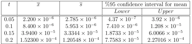
The numerical results have been shown in Table (2), where x and s are error mean and standard deviation of error, respectively.
Table 2: Mean, standard deviation and confidence interval for error mean (T=0.25, m=16)
t x s %95 confidence interval for mean
Lower U pper
0.05 2.200×10⁻⁶ 2.785×10⁻⁶ 4.37×10⁻⁷ 3.92×10⁻⁶ 0.1 8.400×10⁻⁶ 5.953×10⁻⁶ 7.410×10⁻⁶ 1.208×10⁻⁵ 0.15 3.9400×10⁻⁵ 3.3344×10⁻⁵ 1.8733×10⁻⁵ 6.0066×10⁻⁵
6. Conclusion
This paper suggests a computational technique for solving of the nonlinear stochastic differential equation. We use from the stochastic operational matrix based on the NBFs in combination with the collocation technique. The advantage of this method is lower cost of setting up the system of equations without integration, moreover, the computational cost of operations is low. For showing ef-ficiency, the method is applied to some numerical examples. The results show accuracy of the method.
Acknowledgments
The authors are extending their heartfelt thanks to the reviewers for their valuable suggestions for the improvement of the article. Also, the authors thank Islamic Azad University for supporting this work.
References
[1] A. Molabahrami,Integral mean value method for solving a general nonlinear fredholm integro- differential under the mixed conditions,Commun. Numer. Anal. 2013 (2013) 1–15.
[2] B. Oksendal, Stochactic Differential Equations, fifth ed, in: An introduction with applications, Springer-Verlay, New York, 1998.
[3] S. Fadhel and A. Abdulamear,Explicit runge-kutta methods for solving stochastic differential equations, Basrah Researches, 37 (4) (2011).
[4] K. Maleknejad, M. Khodabin and M. Rostami, Numerical solution of stochastic volterra integral equations by stochastic operational matrix based on block pulse functions,Math. Comput. Model. 55 (2012) 791–800.
[5] K. Maleknejad, M. Khodabin and M. Rostami, A numerical method for solving m-dimensional stochastic Itˆ o-volterra integral equations by stochastic operational matrix,Comput. Math. Appl. 63 (2012) 133–143.
[6] M. Khodabin, K. Maleknejad and F. Hosseini,Application of triangular functions to numerical solution of stochas-tic volterra integral equations,IAENG Int. J. Appl. Math., (2013) IJAM-43-1-01.
[7] M. Asgari and F. Hosseini Shekarabi, Numerical solution of nonlinear stochastic differential equations using the block pulse operational matrices,Math. Sci. 7 (2013) 1–5.
[8] R. Ezzati, M. Khodabin and Z. Sadati, Numerical implementation of stochastic operational matrix driven by a fractional Brownian motion for solving a stochastic differential equation, Abst. Appl. Anal., (2014) Hindawi Publishing Corporation.