Sentential Representations in Distributional Semantics

(1)

Sentential Representations in Distributional Semantics

by

The Nghia Pham

Submitted to the Doctoral School in Cognitive and Brain Sciences

in partial fulfillment of the requirements for the degree of

Doctor of Philosophy

at the

UNIVERSITY OF TRENTO

November 2016

c

○

Author . . . .

Doctoral School in Cognitive and Brain Sciences

November 2, 2016

(2)

(3)

Sentential Representations in Distributional Semantics

by

The Nghia Pham

Submitted to the Doctoral School in Cognitive and Brain Sciences on November 2, 2016, in partial fulfillment of the

requirements for the degree of Doctor of Philosophy

Abstract

This thesis is about the problem of representing sentential meaning in distributional seman-tics. Distributional semantics obtains the meanings of words through their usage, based on the hypothesis that words occurring in similar contexts will have similar meanings. In this framework, words are modeled as distributions over contexts and are represented as vec-tors in high dimensional space. Compositional distributional semantics attempts to extend this approach to higher linguistics structures. Some basic composition models proposed in literature to obtain the meaning of phrases or possibly sentences show promising results in modeling simple phrases. The goal of the thesis is to further extend these composition models to obtain sentence meaning representations.

The thesis puts more focus on unsupervised methods which make use of the context of phrases and sentences to optimize the parameters of a model. Three different methods are presented. The first model is the PLF model, a practical composition and linguistically mo-tivated model which is based on the lexical function model introduced by Baroni and Zam-parelli (2010) and Coecke et al. (2010). The second model is the Chunk-based Smoothed Tree Kernels (CSTKs) model, extending Smoothed Tree Kernels (Mehdad et al., 2010) by utilizing vector representations of chunks. The final model is the C-PHRASE model, a neural network-based approach, which jointly optimizes the vector representations of words and phrases using a context predicting objective.

The thesis makes three principal contributions to the field of compositional distribu-tional semantics. The first is to propose a general framework to estimate the parameters and evaluate the basic composition models. This provides a fair way to comparing the models using a set of phrasal datasets. The second is to extend these basic models to the sentence level, using syntactic information to build up the sentence vectors. The third con-tribution is to evaluate all the proposed models, showing that they perform on par with or outperform competing models presented in the literature.

(4)

(5)

Acknowledgments

I would like to thank my advisor, Marco Baroni, for his continuous support during the

course of my PhD. His immense knowledge, creative insight, amazing sense of humor and

endless dedication have helped me in all the time of research and writing of this thesis. I

cannot express enough how much I appreciate his guidance and encouragement throughout

my PhD career.

I would also like to thank my Oversight Committee, Raffaella Bernardi and Roberto

Zamparelli, for all the discussion and invaluable suggestions.

I am indebted to Georgiana Dinu, Angeliki Lazaridou, German Kruszewski, Denis

Pa-perno, Fabio Massimo Zanzotto and Lorenzo Ferrone for their contribution to my work. A

very special thank to them and all the exceptional researchers with whom I had the chance

to collaborate.

Thank you to every member of COMPOSES and the CLICers for creating the most

en-joyable working environment and for the precious feedback. I would also like to express my

gratitude to the ERC 2011 Starting Independent Research Grant n. 283554 (COMPOSES)

for the financial support.

I am grateful to the Doctoral School in Cognitive and Brain Sciences, especially the

head of the school, Francesco Pavani, and the administrator, Leah Mercanti, for their

dedi-cation to the program and the students.

Finally, I thank my family for their unconditional love and tremendous patience; all my

friends, especially Jan Bim, Aidas Aglinskas, Adam Liska, Gergely David, Marco Marelli

and again Georgiana Dinu, Angeliki Lazaridou and German Kruszewski for the wonderful

(6)

(7)

List of Figures

2-1 Neural probablistic language model . . . 21

3-1 FullLex estimation problem. . . 31

3-2 Performance of models on 3 phrasal benchmarks . . . 36

4-1 Function application: If two syntactic sisters have different arity, treat the higher-arity sister as the functor. Compose by multiplying the last matrix in the functor tuple by the argument vector and summing the result to the functor vector. Unsaturated matrices are carried up to the composed node, summing across sisters if needed. . . 43

4-2 Applying function application twice to derive the representation of a tran-sitive sentence. . . 44

5-1 Sample Syntactic Tree . . . 56

5-2 Some Chunk-based Syntactic Sub-Trees of the tree in Figure 5-1 . . . 57

6-1 C-PHRASE context prediction objective for the phrase small cat and its children. The phrase vector is obtained by summing the word vectors. The predicted window is wider for the higher constituent (the phrase). . . 69

A-1 Creating a semantic space. . . 88

A-2 Similarity queries in a semantic space. . . 89

A-3 Creating and using Multiplicative phrase vectors. . . 90

(12)

(13)

List of Tables

2.1 Example vectors in distributional space . . . 20

4.1 Examples of word representations. Subscripts encode, just for mnemonic

purposes, the constituent whose vector the matrix combines with: subject,

object,indirectobject,noun,adjective,verb phrase. . . 43 4.2 Examples of function application. . . 44

4.3 Examples of symmetric composition. . . 44

4.4 The verbto eatassociated to different sets of matrices in different syntactic

contexts. . . 46

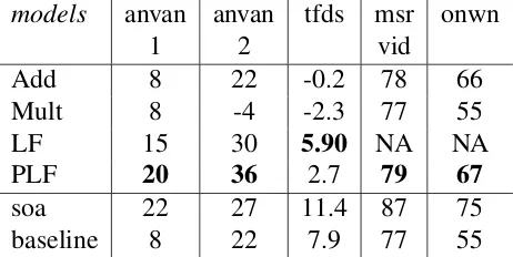
4.5 Performance of composition models on all evaluation sets. Figures of merit

follow previous art on each set and are: percentage Spearman coefficients

for anvan1 and anvan2, t-standardized average difference between mean

cosines with paraphrases and with foils for tfds, percentage Pearson

coef-ficients for msrvid and onwn. . . 50

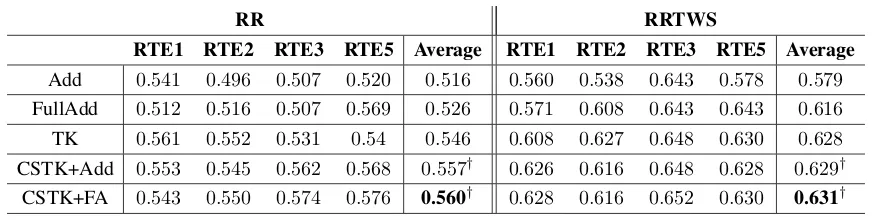
5.1 Task-based analysis: Accuracy on Recognizing Textual Entailment (†is different from both ADD and FullADD with a stat.sig. of𝑝 >0.1.) . . . 63

6.1 Lexical task performance. See Section 6.3.1 for figures of merit (all in

percentage form) and state-of-the-art references. C-BOW results (tuned on

rg) are taken from Baroni et al. 2014b. . . 77

6.2 Sentential task performance. See Section 6.3.1 for figures of merit (all

in percentage form) and state-of-the-art references. The PLF results on

(14)

6.3 Nearest neighbours of neural, network and neural network both for

C-BOW and C-PHRASE . . . 80

A.1 Currently implemented composition functions of inputs(𝑢, 𝑣)together with

parameters and their default values in parenthesis, where defined. Note that

in LF each functor word corresponds to a separate matrix or tensor𝐴𝑢 (Ba-roni and Zamparelli, 2010). . . 91

A.2 Top nearest neighbours ofbelief and offalse belief obtained through

com-position with the FullAdd, LF and Add models. . . 92

A.3 Compositional models for morphology. Top 3 neighbours of florist

us-ing its (low-frequency) corpus-extracted vector, and when the vector is

(15)

Chapter 1

Introduction

Over the past decades, computers have become important assistants for human and kept on

making our jobs faster and easier. They can help us in many tasks ranging from simple

ones like designing circuits to complicated ones like predicting weather or flying airplanes.

Despite being so useful and increasingly powerful, computers are still not able to

under-stand human language and therefore cannot use language as a mean of communication.

Until recently, interaction between human and computers mostly took place through

con-strained interfaces such as keyboards. It has been a great challenge to enable computers to

understand natural languages.

A fundamental aspect of this challenge is how to represent meaning and how to

auto-matically transform natural language into this type of representation. Traditionally, formal

semantics has attempted to represent language utterances such as sentences as logic

for-mulas (Montague, 1970). The meaning of a sentence such as "every student left"can be

represented as the following first order logic formula

∀𝑥(𝑠𝑡𝑢𝑑𝑒𝑛𝑡(𝑥)→𝑙𝑒𝑓 𝑡(𝑥))

This type of representation is quite attractive since it allows automatic reasoning. For

example: given thatevery student left, ∀𝑥(𝑠𝑡𝑢𝑑𝑒𝑛𝑡(𝑥) → 𝑙𝑒𝑓 𝑡(𝑥)), andJohn is a student,

𝑠𝑡𝑢𝑑𝑒𝑛𝑡(𝐽 𝑜ℎ𝑛), using logic tools, a computer can deduce thatJohn left, 𝑙𝑒𝑓 𝑡(𝐽 𝑜ℎ𝑛).

For-mal semantics also introduces methods, such as lambda calculus, for building the meaning

of sentences compositionally based on their components.

(16)

the words themselves and it has no way to obtain the relationship between words from the

data. For instance, formal semantics cannot learn thatmurder →killsordislikeis similar tohate. Although this type of information can be manually encoded, this limitation highly

restricts the use of formal semantics in practical applications.

Distributional semantics, on the contrary, can learn the relationship between words from

increasingly available text corpora (Turney and Pantel, 2010; Erk, 2012; Clark, 2015). It

is based on the distributional hypothesis "Words that appear in similar contexts tend to

have similar meanings" (Miller and Charles, 1991). Given a text corpus, distributional

semantics can build the meaning of words as co-occurrence vectors and, based on this type

of representation, it can tell how similar words are to each other. This is very useful because

assessing similarity in meaning is central to many language technology applications such

as question answering or information retrieval.

However, historically, there has been no obvious way to extract the meaning of

lin-guistic utterance beyond words. Unlike formal semantics, distributional semantics lacks a

framework to construct the meaning of phrases and sentences based on their components.

The question of assessing meaning similarity above the word level within the distributional

paradigm has received a lot of attention in recent years (Mitchell and Lapata, 2008, 2010;

Zanzotto et al., 2010; Guevara, 2010; Baroni and Zamparelli, 2010; Coecke et al., 2010).

A number of compositional frameworks have been proposed in the literature, each of these

defining operations to combine word vectors into representations for more complex

struc-tures such as phrases. However, these works pay more attention to simple phrases, e.g.

adjective noun construction, with limited experiments at the sentence level. This thesis

focus on how to obtain vectors for sentences using distributional methods, as sentences

are the basic language structure that human uses to interact with each other. Moreover, It

looks at how information such as syntactic structure can be incorporated into the process

of building sentence representations.

In chapter 2, I begin with an overview of distributional semantics. I discuss the two

general ways of obtaining word vectors from the literature: using co-occurrence count

and predicting the context. Also, I will briefly go over the composition models in the

(17)

range from simple parameter-free models like addition to complex models involving tensor

multiplication and estimation.

Chapter 3 takes a more thorough look at these composition models. First, I introduce

a general and effective method for estimating the parameters of every composition model.

Then, based on this estimation method, I describe a truly fair way to compare all the models

I consider using a variety of phrase datasets. This chapter is of great importance since,

based on the results presented in it, we can see which models are more effective in building

phrasal vectors, that thus can further be adapted to derive sentential vectors.

The rest of this thesis will focus on methods to achieve the goal of obtain meaning

representation of sentences. These methods are very different from each other but are built

using the same building blocks: simple composition models.

Chapter 4 describes the practical lexical function (PLF), a purely compositional method,

which is based on the lexical function model introduced by Baroni and Zamparelli (2010)

and Coecke et al. (2010). This lexical function model is inspired by the function

applica-tion view of composiapplica-tion that is common in formal semantics. In this model, nouns are

represented as vectors, adjectives are matrices that modify the meaning of a noun by

trans-forming its vector to another vector. Other content words such as transitive verbs or adverb

are represented as high-order tensors. In PLF, high order tensors are avoided and replaced

with multiple matrices, therefore problems inherent to the lexical function model such as

data sparseness and highly complex computation are avoided while other attractive features

like syntax-sensitive are maintained.

Another method, which is introduced in chapter 5, is a combination of tree kernels

and basic composition. Syntactic tree kernels are powerful tools, which use the set of

subtrees of the syntactic tree of a sentence as its vector representation. Using this type of

representation, task-specific similarity between sentences are learned by assigning weights

to the syntactic subtrees. An disadvantage of this method is the lack of a way to merge

similar subtrees using the similarity betweens words and simple phrases, which is nicely

supplied by the basic composition models.

Finally, in chapter 6, I present C-PHRASE, another alternative to obtain sentence vector

(18)

et al. (2013c), two very efficient methods to obtain good word vector representation. By

incorporating syntactic information into the objective function, the C-PHRASE model is

able to learn word and phrase vectors jointly. It does not only improve the quality of

the word vectors but also obtain good sentence vectors which are then tested on several

sentential task such as textual similarity, entailment and sentiment analysis.

Additionally, in the appendix A, I describes the practical tools I have built during the

course of this thesis, which are put together to form the DISSECT toolkit. The toolkit is

written in Python, a high-level, general purpose programming language, which is popular

in the NLP community. The toolkit consists of a set of ways to build word vectors from

co-occurrence counts, methods to combine them into phrase or sentence vectors and to

estimate the parameters for those models. It is highly extensible, which hopefully will

be useful for researchers who are interested in distributional semantics in general or more

(19)

Chapter 2

Background

2.1

Distributional Semantics

The need to assess similarity in meaning is central to many language technology

applica-tions, and distributional methods are the most robust approach to the task. These methods

measure word similarity based on patterns of occurrence in large corpora, following the

intuition that similar words occur in similar contexts. More precisely, vector space models,

the most widely used distributional models, represent words as high-dimensional vectors,

where the dimensions represent (functions of) context features, such as co-occurring

con-text words. The relatedness of two words is assessed by comparing their vector

represen-tations.

There are two prominent approaches in distributional semantics to obtain the word

vec-tors. The traditional approach, which is calledcount model(Baroni et al., 2014), is a direct

realization of the distributional hypothesis where the context features are the words that

co-occur with the target words. The more recent approach, which is referred aspredictmodel

(Baroni et al., 2014), can be seen as a more indirect realization of the distributional

hypoth-esis. In this approach the word vectors are typically learned by predicting the context, e.g.

(20)

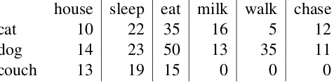
house sleep eat milk walk chase

cat 10 22 35 16 5 12

dog 14 23 50 13 35 11

couch 13 19 15 0 0 0

Table 2.1: Example vectors in distributional space

2.1.1

Count model

In count models, to obtain the word vectors, the first step is to select a fixed set of

con-texts, which are typically the most common content words (e.g. nouns, verbs, adjectives,

adverbs). These words are used as the dimension of the vectors in the high-dimensional

space. Then, (a function of) the the number of times the target word occurs with a given

context word is computed and used as the value of the corresponding dimension. Table 2.1

illustrates some of the vectors in such a semantic space.

Normally, vectors with raw frequency (without applying a frequency weighting

func-tion) do not perform well in practical applications since the dimensions corresponding to

frequent context words, which contribute little to the meaning of other words, tend to have

the highest values dominating other dimensions. Weighting schemes are therefore used

to lessen the effect of highly frequent context words. Some popular weighting schemes

include TF-IDF (Salton, 1979), pointwise mutual information (PMI) (Church and Hanks,

1990).

𝑝𝑚𝑖(𝑥, 𝑦) = 𝑙𝑜𝑔 𝑝(𝑥, 𝑦)

𝑝(𝑥)𝑝(𝑦) (2.1)

Other weighting schemes inspired by PMI are positive pointwise mutual information

PPMI or local mutual information (LMI) (Bullinaria and Levy, 2007; Evert, 2005).

To reduce the number of dimension in the vector space, thus reducing the amount of

computation, methods such as truncated SVD (Golub and Van Loan, 1996) or NMF (Lee

and Seung, 1999) are used. SVD, singular value decomposition, factorizes an matrix M

(21)

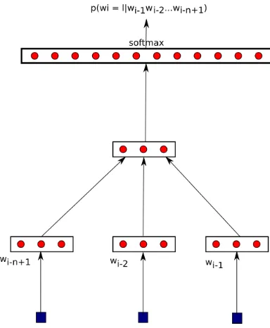
Figure 2-1: Neural probablistic language model

factorized into two non-negative matricesM=W*H, andWis used in place ofM. These dimensionality reduction methods can also have a side effect of reducing noises from the

corpus thus resulting in semantic space with higher quality.

2.1.2

Predict model

As the name suggests, predict models learn word vectors by using them to predict the

context. In these models, the dimensions in a word vector are trained to maximize the

probability of the contexts where the word is observed in the corpus. Because similar

words occur in similar contexts, similar vectors are naturally assigned to similar words.

One of the first predict models was the neural language model. The main goal of

lan-guage modeling is to predict the current word given the history (all the words before the

current word). An early neural network for language modeling by Bengio et al. (2003) is

presented in figure 2-1. Here words are presented as low-dimension vectors and a

func-tion based on the presentafunc-tion of the last n words is used to compute the distribufunc-tion of the

words that occur after them. The word vector representations obtained from these methods,

despite originally being a byproduct, are a good proxy of word meaning.

(22)

some notable models being those presented by Collobert and Weston (2008); Collobert

et al. (2011); Huang et al. (2012); Turian et al. (2010).

One of the most influential works in this direction is Mikolov et al. (2013c), where

the authors introduce two very simple and efficient method to obtain good word meaning

representation: the Skip-gram and C-BOW models. The Skip-gram model derives the vector of a target word by setting its weights to predict the words surrounding it in the

corpus. More specifically, the objective function is:

1

𝑇

𝑇 ∑︁

𝑡=1

∑︁

−𝑐≤𝑗≤𝑐,𝑗̸=0

log𝑝(𝑤𝑡+𝑗|𝑤𝑡) (2.2) where the word sequence𝑤1, 𝑤2, ..., 𝑤𝑇 is the training corpus and𝑐is the size of the

win-dow around the target word𝑤𝑡, consisting of the context words𝑤𝑡+𝑗that must be predicted by the induced vector representation for the target.

While Skip-gram learns the word vector by using the target word to predict the

sur-rounding words, C-BOW, on the other hand, uses the combination of the surround words

to predict the word in the middle. The objective function is:

1

𝑇

𝑇 ∑︁

𝑡=1

log𝑝(𝑤𝑡|𝑤𝑡−𝑐..𝑤𝑡−1, 𝑤𝑡+1..𝑤𝑡+𝑐) (2.3) Despiting being very simple, Skip-gram and C-BOW models obtain extremely high

quality vectors. They achieved the state of the art results in several lexical tasks, including

the word analogy task (Mikolov et al., 2013c) where given a pair exemplifying a relation

(boy/son) and a test word (girl); they can find the word (daughter) that instantiates the same

relation with the test word as that of the example pair.

2.2

Compositional models

The vector representations provided by distributional semantic models are very useful in

applications that require a representation of word meaning in general, or in particular

re-quire an measure of similarity between word meanings. Examples of such applications

(23)

(Du-mais, 2003; Turney and Pantel, 2010). However, these models cannot be used directly to

obtain the meaning representations for complex phrases or sentences since there are

un-limited number of possible sentences and few of them occur frequently enough in text

corpora in order for distributional methods to obtain a reliable vector representation. In

re-cent year, the question of obtaining semantic representationabove the word levelwithin the

distributional paradigm has received a lot of attention (Mitchell and Lapata, 2008, 2010;

Grefenstette and Sadrzadeh, 2011a; Guevara, 2010; Zanzotto et al., 2010). Most work

deal-ing with this question relies on the compositionality of languages, in which the meandeal-ing

of an utterance can be represented as a combination of the meaning of its parts. A number

of compositional frameworks have been proposed in the literature, each of these defining

operations to combine word vectors into representations for phrases or even sentences.

Being probably the most notable work on the topic, Mitchell and Lapata (2010) have

proposed several classes of composition models. The first method, also the most intuitive

way to compose the phrase vector from its component words, is by summing its word

vectors. This model is called additive model (Add)

→

𝑝 =→𝑢+→𝑣 (2.4)

where→𝑝 is the vector of the phrase and→𝑢and→𝑣 are the vectors of its component words.

An extension of this model is the weighted additive model (WAdd), where the

contri-bution of the components are determined by the two pre-defined weights

→

𝑝 =𝑤1

→

𝑢+𝑤2

→

𝑣 (2.5)

Note that if𝑤1 =𝑤2 = 1, WAdd becomes the simple Add model.

Another simple alternative to additive is the multiplicative modelMult, which utilizes

the pointwise multiplication operation

→

𝑝 =→𝑢⊙→𝑣 (2.6)

Both addition and multiplication are commutative, thus making simple additive and

(24)

There-fore,pandas eat bambooandbamboo eats pandaswill have the same meaning

representa-tion for these models.

Another model proposed by Mitchell and Lapata (2010), the dilation model, is

asym-metric. First the vector→𝑣 is decomposed into 2 components, one is parallel to →𝑢 and the

other is orthogonal to→𝑢. The component parallel to u is then stretched with a weight𝜆and

then recombined with the other component so that the final vector is more similar to→𝑢.

→

𝑝 =||→𝑢||2 2

→

𝑣 + (𝜆−1)⟨→𝑢,→𝑣⟩→𝑢 (2.7) Guevara (2010) and Zanzotto et al. (2010) introduce the full additive (FullAdd) model,

a similar model to WAdd but replacing the scalar weights with matrices.

→

𝑝 =W1

→

𝑢+W2

→

𝑣 (2.8)

All the models above were inspired by mathematical operations on vectors with little

insight from linguistics. Baroni and Zamparelli (2010) and Coecke et al. (2010) introduce

the lexical function model (LF), which follows the function application intuition of formal

semantics, where a noun is a set of entities and an adjective is a function that maps a set of

entities to another set. Here, a noun is represented as a vector and an adjective is a matrix

that maps a vector to another.

→

𝑝 =A𝑢

→

𝑣 (2.9)

This model can also be generalized to other parts of speech, e.g. a transitive verb can

be represented as a 3-order tensor that maps a pair of vectors to a vector.

The last model, introduced by Socher et al. (2012) is a neural network-based

general-ization of LF. In this model, every word is represented as a matrix and a vector ([A𝑤,

→

𝑤]),

and the composition function is:

→

𝑝 =𝑡𝑎𝑛ℎ

(︃ M [︃ A𝑢 → 𝑣 A𝑣 → 𝑢 ]︃)︃ (2.10)

(25)

The composition models discussed in this chapter lay a good foundation for obtaining

semantic representation of sentences. However, in order to achieve this goal, we must

perform a systematic comparison between the model in order to evaluate their strengths

and weaknesses, thus enabling us to select the most promising model to further develop

it into a good model to obtain sentential meaning. In chapter 3 and 4, I will present my

(26)

(27)

Chapter 3

General Parameter Estimation and

Evaluation of Basic Composition Models

3.1

Introduction

The question of assessing meaning similarityabove the word levelwithin the distributional

paradigm has received a lot of attention in recent years. A number of compositional

frame-works have been proposed in the literature, each of these defining operations to combine

word vectors into representations for phrases. These models are briefly discussed in

chap-ter 2 and range from simple but robust methods such as vector addition to more advanced

methods, such as learning function words as tensors and composing constituents through

inner product operations.

Empirical evaluations in which alternative methods are tested in comparable settings

are thus called for. This is complicated by the fact that the proposed compositional

frame-works package together a number of choices that are conceptually distinct, but difficult to

disentangle. Broadly, these concern:

(i) the input representations fed to composition; (ii) the composition operation proper;

(iii) the method to estimate the parameters of the composition operation.

For example, Mitchell and Lapata in their classic 2010 study propose a set of

composi-tion operacomposi-tions (multiplicative, additive, etc.), but they also experiment with two different

(28)

distribu-tions over latent topics) and use supervised training via a grid search over parameter

set-tings to estimate their models. Guevara (2010), to give just one further example, is not only

proposing a different composition method with respect to Mitchell and Lapata, but he is

also adopting different input vectors (word co-occurrences compressed via SVD) and an

unsupervised estimation method based on minimizing the distance of composed vectors to

their equivalents directly extracted from the source corpus.

Blacoe and Lapata (2012) have recently highlighted the importance of teasing apart the

different aspects of a composition framework, presenting an evaluation in which different

input vector representations are crossed with different composition methods. However,

two out of three composition methods they evaluate are parameter-free, so that they can

side-step the issue of fixing the parameter estimation method.

In this chapter, I evaluate all composition methods I know of, excluding a few that

lag behind the state of the art or are special cases of those I consider, while keeping the

estimation method constant. This evaluation is made possible by our extension to all

tar-get composition models of the corpus-extracted phrase approximation method originally

proposed inad-hocsettings by Baroni and Zamparelli (2010) and Guevara (2010).

For the models for which it is feasible, I compare the phrase approximation approach

to supervised estimation with crossvalidation, and show that phrase approximation is

com-petitive, thus confirming that I am not comparing models under poor training conditions.

Our tests are conducted over three tasks that involve different syntactic constructions and

evaluation setups. Finally, I consider a range of parameter settings for the input vector

representations, to insure that our results are not too brittle or parameter-dependent.

3.2

Least-squares model estimation using corpus-extracted

phrase vectors

(29)

the following Frobenius norm notation: ||𝑋||𝐹 = ⟨𝑋, 𝑋⟩1/2. Vectors are assumed to be column vectors and I use 𝑥𝑖 to stand for the𝑖-th (𝑚×1)-dimensional column of matrix

𝑋. I use [𝑋, 𝑌] ∈ R𝑚×2𝑛 _{to denote the horizontal concatenation of two matrices while} [︀𝑋

𝑌 ]︀

∈R2𝑚×𝑛_{is their vertical concatenation.}

General problem statement I assume vocabularies of constituents𝒰, 𝒱 and that of re-sulting phrases𝒫. The training data consist of a set of tuples(𝑢, 𝑣, 𝑝)where𝑝stands for the phrase associated to the constituents𝑢and𝑣:

𝑇 ={(𝑢𝑖, 𝑣𝑖, 𝑝𝑖)|(𝑢𝑖, 𝑣𝑖, 𝑝𝑖)∈ 𝒰 × 𝒱 × 𝒫,1≤𝑖≤𝑘}

I build the matrices 𝑈, 𝑉, 𝑃 ∈ R𝑚×𝑘 _{by concatenating the vectors associated to the} training data elements as columns.1

Given the training data matrices, the general problem can be stated as:

𝜃* = arg min

𝜃

||𝑃 −𝑓 𝑐𝑜𝑚𝑝𝜃(𝑈, 𝑉)||𝐹

where 𝑓 𝑐𝑜𝑚𝑝𝜃 is a composition function and 𝜃 stands for a list of parameters that this

composition function is associated to. The composition functions are defined: 𝑓 𝑐𝑜𝑚𝑝𝜃 :

R𝑚×1_×_R𝑚×1 _→_R𝑚×1_and_{𝑓 𝑐𝑜𝑚𝑝}

𝜃(𝑈, 𝑉)stands for their natural extension when applied

on the individual columns of the𝑈 and𝑉 matrices.

WAdd The weighted additive model returns the sum of the composing vectors which have been re-weighted by some scalars𝑤1and𝑤2:

→

𝑝 =𝑤1

→

𝑢+𝑤2

→

𝑣. The problem becomes:

𝑤₁*, 𝑤₂* = arg min

𝑤1,𝑤2∈R

||𝑃 −𝑤1𝑈 −𝑤2𝑉||𝐹 The optimal𝑤1 and𝑤2are given by:

𝑤*₁ = ||𝑉||

2

𝐹⟨𝑈, 𝑃⟩ − ⟨𝑈, 𝑉⟩⟨𝑉, 𝑃⟩

||𝑈||2

𝐹||𝑉||2𝐹 − ⟨𝑈, 𝑉⟩2

(3.1)

(30)

𝑤*₂ = ||𝑈||

2

𝐹⟨𝑉, 𝑃⟩ − ⟨𝑈, 𝑉⟩⟨𝑈, 𝑃⟩

||𝑈||2

𝐹||𝑉||2𝐹 − ⟨𝑈, 𝑉⟩2

(3.2)

Dil Given two vectors →𝑢 and →𝑣, the dilation model computes the phrase vector →𝑝 =

||→𝑢||2→_𝑣 _{+ (}_𝜆₋₁₎_⟨→_𝑢,→_𝑣_⟩→_𝑢 _{where the parameter}_𝜆_{is a scalar. The problem becomes:} 𝜆* = arg min

𝜆∈R

||𝑃 −𝑉 𝐷||𝑢𝑖||2 −𝑈 𝐷(𝜆−1)⟨𝑢𝑖,𝑣𝑖⟩||𝐹

where by𝐷||𝑢𝑖||2 and𝐷(𝜆−1)⟨𝑢𝑖,𝑣𝑖⟩ I denote diagonal matrices with diagonal elements(𝑖, 𝑖)

given by||𝑢𝑖||2 and(𝜆−1)⟨𝑢𝑖, 𝑣𝑖⟩respectively. The solution is:

𝜆* = 1−

∑︀𝑘

𝑖=1⟨𝑢𝑖,(||𝑢𝑖|| 2_𝑣

𝑖−𝑝𝑖)⟩⟨𝑢𝑖, 𝑣𝑖⟩ ∑︀𝑘

𝑖=1⟨𝑢𝑖, 𝑣𝑖⟩2||𝑢𝑖||2

Mult Given two vectors→𝑢and→𝑣, the weighted multiplicative model computes the phrase vector→𝑝 = →𝑢𝑤1 ⊙→𝑣𝑤2 where⊙stands for component-wise multiplication. I assume for this model that𝑈, 𝑉, 𝑃 ∈ R𝑚₊₊×𝑛, i.e. that the entries are strictly larger than 0: in practice I add a small smoothing constant to all elements to achieve this (Mult performs badly on

negative entries, such as those produced by SVD). I use the 𝑤1 and 𝑤2 weights obtained

when solving the much simpler related problem:2

𝑤*₁, 𝑤*₂ = arg min

𝑤1,𝑤2∈R

||𝑙𝑜𝑔(𝑃)−𝑙𝑜𝑔(𝑈.∧𝑤1⊙𝑉.∧𝑤2)||𝐹

where.∧ stands for the component-wise power operation. The solution is the same as that

for WAdd, given in equations (1) and (2), with 𝑈 → 𝑙𝑜𝑔(𝑈), 𝑉 → 𝑙𝑜𝑔(𝑉) and 𝑃 →

𝑙𝑜𝑔(𝑃).

FullAdd The full additive model assumes the composition of two vectors to be →𝑝 =

𝑊1

→

𝑢+𝑊2

→

𝑣 where𝑊1, 𝑊2 ∈R𝑚×𝑚. The problem is:

[𝑊1, 𝑊2]* = arg min [𝑊1,𝑊2]∈R𝑚×2𝑚

||𝑃 −[𝑊1𝑊2] [︂

𝑈 𝑉

]︂

||

(31)

This is a multivariate linear regression problem (Hastie et al., 2009) for which the least

squares estimate is given by: [𝑊1, 𝑊2] = ((𝑋𝑇𝑋)−1𝑋𝑇𝑌)𝑇 where I use 𝑋 = [𝑈𝑇, 𝑉𝑇]

and𝑌 =𝑃𝑇_.

LF The lexical function composition method learns a matrix representation for each func-tor (given by 𝒰 here) and defines composition as matrix-vector multiplication. More pre-cisely:→𝑝 =𝐴𝑢

→

𝑣 where𝐴𝑢is a matrix associated to each functor𝑢∈ 𝒰. I denote by𝑇𝑢the training data subset associated to an element𝑢, which contains only tuples which have𝑢as

first element. Learning the matrix representations amounts to solving the set of problems:

𝐴𝑢 = arg min 𝐴𝑢∈R𝑚×𝑚

||𝑃𝑢 −𝐴𝑢𝑉𝑢||

for each𝑢∈ 𝒰 where𝑃𝑢, 𝑉𝑢 ∈ R𝑚×|𝑇𝑢|are the matrices corresponding to the𝑇𝑢 training subset. The solutions are given by: 𝐴𝑢 = ((𝑉𝑢𝑉𝑢𝑇)−1𝑉𝑢𝑃𝑢𝑇)𝑇. This composition function

does not use the functor vectors.

FullLex This model can be seen as a generalization of LF which makes no assumption on which of the constituents is a functor, so that both words get a matrix and a vector

representation. The composition function is:

→

𝑝 =𝑡𝑎𝑛ℎ([𝑊1, 𝑊2] [︃ 𝐴𝑢 → 𝑣 𝐴𝑣 → 𝑢 ]︃ )

where 𝐴𝑢 and 𝐴𝑣 are the matrices associated to constituents 𝑢 and 𝑣 and [𝑊1, 𝑊2] ∈

R𝑚×2𝑚_{. The estimation problem is given in Figure 3-1.}

𝑊₁*, 𝑊₂*, 𝐴*_𝑢₁, ..., 𝐴*_𝑣₁, ...= arg min

R𝑚×𝑚

||𝑎𝑡𝑎𝑛ℎ(𝑃𝑇)−[𝑊1, 𝑊2] [︃

[𝐴𝑢1

→

𝑣1, ..., 𝐴𝑢𝑘

→

𝑣𝑘]

[𝐴𝑣1

→

𝑢1, ..., 𝐴𝑣𝑘

→

𝑢𝑘] ]︃

||𝐹

= arg min

R𝑚×𝑚

||𝑎𝑡𝑎𝑛ℎ(𝑃𝑇)−𝑊1[𝐴𝑢1

→

𝑣1, ..., 𝐴𝑢𝑘

→

𝑣𝑘]−𝑊2[𝐴𝑣1

→

𝑢1, ..., 𝐴𝑣𝑘

→

𝑢𝑘]||𝐹 Figure 3-1: FullLex estimation problem.

(32)

a block coordinate descent method, in which I fix each of the matrix variables but one and

solve the corresponding least-squares linear regression problem, for which I can use the

closed-form solution. Fixing everything but[𝑊1, 𝑊2]:

[𝑊₁*, 𝑊₂*] = ((𝑋𝑇𝑋)−1𝑋𝑇𝑌)𝑇

𝑋 =

[︃

[𝐴𝑢1

→

𝑣1, ..., 𝐴𝑢𝑘

→

𝑣𝑘]

[𝐴𝑣1

→

𝑢1, ..., 𝐴𝑣𝑘

→

𝑢𝑘] ]︃𝑇

𝑌 =𝑎𝑡𝑎𝑛ℎ(𝑃𝑇)

Fixing everything but𝐴𝑢 for some element𝑢, the objective function becomes:

||𝑎𝑡𝑎𝑛ℎ(𝑃𝑢)−𝑊1𝐴𝑢𝑉𝑢−𝑊2[𝐴𝑣1

→

𝑢, ..., 𝐴𝑣𝑘′

→

𝑢]||𝐹

where𝑣1...𝑣𝑘′ ∈ 𝒱 are the elements occurring with𝑢in the training data and𝑉_𝑢 the matrix

resulting from their concatenation. The update formula for the𝐴𝑢 matrices becomes:

𝐴*_𝑢 =𝑊₁−1((𝑋𝑇𝑋)−1𝑋𝑇𝑌)𝑇

𝑋 =𝑉_𝑢𝑇

𝑌 = (𝑎𝑡𝑎𝑛ℎ(𝑃𝑢)−𝑊2[𝐴𝑣1

→

𝑢, ..., 𝐴𝑣𝑘′

→

𝑢])𝑇

In all the experiments, FullLex estimation converges after very few passes though the

matrices. Despite the very large number of parameters of this model, when evaluating on

the test data I observe that using a higher dimensional space (such as 200 dimensions) still

performs better than a lower dimensional one (e.g., 50 dimensions).

3.3

Evaluation setup and implementation

3.3.1

Datasets

I evaluate the composition methods on three phrase-based benchmarks that test the models

(33)

Intransitive sentences The first dataset, introduced by Mitchell and Lapata (2008), fo-cuses on simple sentences consisting of intransitive verbs and their noun subjects. It

con-tains a total of 120 sentence pairs together with human similarity judgments on a 7-point

scale. For example, conflict erupts/conflict bursts is scored 7, skin glows/skin burns is

scored 1. On average, each pair is rated by 30 participants. Rather than evaluating against

mean scores, I use each rating as a separate data point, as done by Mitchell and Lapata. I

report Spearman correlations between human-assigned scores and model cosine scores.

Adjective-noun phrases Turney (2012) introduced a dataset including both noun-noun compounds and adjective-noun phrases (ANs). I focus on the latter, and I frame the task

differently from Turney’s original definition due to data sparsity issues.3 _{In our version, the}

dataset contains 620 ANs, each paired with a single-noun paraphrase. Examples include:

archaeological site/dig, spousal relationship/marriageanddangerous

undertaking/adven-ture. I evaluate a model by computing the cosine of all 20K nouns in our semantic space

with the target AN, and looking at the rank of the correct paraphrase in this list. The lower

the rank, the better the model. I report median rank across the test items.

Determiner phrases The last dataset, introduced in Bernardi et al. (2013), focuses on a class of grammatical terms (rather than content words), namely determiners. It is a

multiple-choice test where target nouns (e.g., amnesia) must be matched with the most

closely related determiner(-noun) phrases (DPs) (e.g., no memory). The task differs from

the previous one also because here the targets are single words, and the related items are

composite. There are 173 target nouns in total, each paired with one correct DP response,

as well as 5 foils, namely the determiner (no) and noun (memory) from the correct

re-sponse and three more DPs, two of which contain the same noun as the correct phrase (less

memory, all memory), the third the same determiner (no repertoire). Other examples of

targets/related-phrases are polysemy/several senses and trilogy/three books. The models

compute cosines between target noun and responses and are scored based on their accuracy

3_{Turney used a corpus of about 50 billion words, almost 20 times larger than ours, and I have very}

(34)

at ranking the correct phrase first.

3.3.2

Input vectors

I extracted distributional semantic vectors using as source corpus the concatenation of

ukWaC, Wikipedia (2009 dump) and BNC, 2.8 billion tokens in total.4 I use a

bag-of-words approach and I count co-occurrences within sentences and with a limit of maximally

50 words surrounding the target word. By tuning on the MEN lexical relatedness dataset,5

I decided to use the top 10K most frequent content lemmas as context features (vs. top 10K

inflected forms), and I experimented with positive Pointwise and Local Mutual Information

(Evert, 2005) as association measures (vs. raw counts, log transform and a probability ratio

measure) and dimensionality reduction by NMF (Lee and Seung, 2000) and SVD (Golub

and Van Loan, 1996) (both outperforming full dimensionality vectors on MEN). For both

reduction techniques, I varied the number of dimensions to be preserved from 50 to 300 in

50-unit intervals. As Local Mutual Information performed very poorly across composition

experiments and other parameter choices, I dropped it. I will thus report, for each

experi-ment and composition method, the distribution of the relevant performance measure across

12 input settings (NMF vs. SVD times 6 dimensionalities). However, since the Mult model,

as expected, worked very poorly when the input vectors contained negative values, as is the

case with SVD, for this model I report result distributions across the 6 NMF variations

only.

3.3.3

Composition model estimation

Training by approximating the corpus-extracted phrase vectors requires corpus-based

ex-amples of input (constituent word) and output (phrase) vectors for the composition

pro-cesses to be learned. In all cases, training examples are simply selected based on corpus

frequency. For the first experiment, I have 42 distinct target verbs and a total of ≈20K training instances, that is,⟨⟨noun,verb⟩,noun-verb⟩tuples (505 per verb on average). For

4_{http://wacky.sslmit.unibo.it}_;

http://www.natcorp.ox.ac.uk

5

(35)

the second experiment, I have 479 adjectives and≈1 million⟨⟨adjective,noun⟩, adjective-noun⟩training tuples (2K per adjective on average). In the third, 50 determiners and 50K

⟨⟨determiner,noun⟩, determiner-noun⟩tuples (1K per determiner). For all models except LF and FullLex, training examples are pooled across target elements to learn a single set of

parameters. The LF model takes only argument word vectors as inputs (the functors in the

three datasets are verbs, adjectives and determiners, respectively). A separate weight

ma-trix is learned for each functor, using the corresponding training data.6 The FullLex method

jointly learns distinct matrix representations for both left- and right-hand side constituents.

For this reason, I must train this model on balanced datasets. More precisely, for the

in-transitive verb experiments, I use training data containing noun-verb phrases in which the

verbs and the nouns are present in the lists of 1,500 most frequent verbs/nouns respectively,

adding to these the verbs and nouns present in our dataset. I obtain 400K training tuples.

I create the training data similarity for the other datasets obtaining 440K adjective-noun

and 50K determiner phrase training tuples, respectively (I also experimented with FullLex

trained on the same tuples used for the other models, obtaining considerably worse results

than those reported). Finally, for Dil I treat direction of stretching as a further parameter to

be optimized, and find that for intransitives it is better to stretch verbs, in the other datasets

nouns.

For the simple composition models for which parameters consist of one or two scalars,

namely WAdd, Mult and Dil, I also tune the parameters through 5-fold crossvalidation on

the datasets, directly optimizing the parameters on the target tasks. For WAdd and Mult, I

search𝑤1,𝑤2 through the crossproduct of the interval [0 : 5]in0.2-sized steps. For Dil I

use𝜆 ∈[0 : 20], again in0.2-sized steps.

3.4

Evaluation results

6_{For the LF model I have experimented with least squeares regression with and without regularization,}

obtaining similar results.

8_{For intransitive sentences, figure of merit is Spearman correlation, for ANs median rank of correct}

(36)

Add Dil Mult Fulladd Le xfunc Fullle x Cor pus 0.00 0.05 0.10 0.15 0.20 0.25 0.30 Intransitive sentences ● ● ● ● ●

Add Dil Mult

Fulladd Le xfunc Fullle x Cor pus 1000 800 600 400 200 ANs ● ●

Add Dil Mult

Fulladd Le xfunc Fullle x Cor pus 0.15 0.20 0.25 0.30 0.35 DPs

Figure 3-2: Boxplots displaying composition model performance distribution on three benchmarks, across input vector settings (6 datapoints for Mult, 12 for all other models).8

I begin with some remarks pertaining to the overall quality of and motivation for

corpus-phrase-based estimation. In seven out of nine comparisons of this unsupervised technique

with fully supervised crossvalidation (3 “simple” models –WAdd, Dil and Mult– times 3

test sets), there was no significant difference between the two estimation methods.9

Super-vised estimation outperformed the corpus-phrase-based method only for Dil on the

intran-sitive sentence and AN benchmarks, but crossvalidated Dil was outperformed by at least

one phrase-estimated simple model on both benchmarks.

The rightmost boxes in the panels of Figure 3-2 depict the performance distribution for

using phrase vectors directly extracted from the corpus to tackle the various tasks. This

non-compositional approach outperforms all non-compositional methods in two tasks over three,

and it is one of the best approaches in the third, although in all cases even its top scores

are far from the theoretical ceiling. Still, performance is impressive, especially in light of

the fact that the non-compositional approach suffers of serious data-sparseness problems.

Performance on the intransitive task is above state-of-the-art despite the fact that for almost

half of the cases one test phrase is not in the corpus, resulting in 0 vectors and consequently

0 similarity pairs. The other benchmarks have better corpus-phrase coverage (nearly perfect

AN coverage; for DPs, about 90% correct phrase responses are in the corpus), but many

(37)

target phrases occur only rarely, leading to unreliable distributional vectors. I interpret these

results as a good motivation for corpus-phrase-based estimation. On the one hand they

show how good these vectors are, and thus that they are sensible targets of learning. On the

other hand, they do not suffice, since natural language is infinitely productive and thus no

corpus can provide full phrase coverage, justifying the whole compositional enterprise.

The other boxes in Figure 3-2 report the performance of the composition methods

trained by corpus phrase approximation. Nearly all models are significantly above chance

in all tasks, except for FullAdd on intransitive sentences. To put AN median ranks into

perspective, consider that a median rank as high as 8,300 has near-0 probability to occur

by chance. For DP accuracy, random guessing gets 0.17% accuracy.

LF emerges consistently as the best model. On intransitive constructions, it significantly

outperforms all other models except Mult, but the difference approaches significance even

with respect to the latter (𝑝 = 0.071). On this task, LF’s median correlation (0.26) is

nearly equivalent to thebestcorrelation across a wide range of parameters reported by Erk

and Padó (2008) (0.27). In the AN task, LF significantly outperforms FullLex and Dil and,

visually, its distribution is slightly more skewed towards lower (better) ranks than any other

model. In the DP task, LF significantly outperforms WAdd and Mult and, visually, most of

its distribution lies above that of the other models. Most importantly, LF is the only model

that is consistent across the three tasks, with all other models displaying instead a brittle

performance pattern.10

Still, the top-performance range of all models on the three tasks is underwhelming, and

none of them succeeds in exploiting compositionality to do significantly better than using

whatever phrase vectors can be extracted from the corpus directly. Clearly, much work is

still needed to develop truly successful cDSMs.

The AN results might look particularly worrying, considering that even the top

(low-est) median ranks are above 100. A qualitative analysis, however, suggests that the actual

performance is not as bad as the numerical scores suggest, since often the nearest

neigh-bours of the ANs to be paraphrased are nouns that are as strongly related to the ANs as

10_{No systematic trend emerged pertaining to the input vector parameters (SVD vs. NMF and retained}

(38)

the gold standard response (although not necessarily proper paraphrases). For example, the

gold response to colorimetric analysisiscolorimetry, whereas the LF (NMF, 300

dimen-sions) nearest neighbour ischromatography; the gold response toheavy particleisbaryon,

whereas LF proposesmuon; formelodic phrasethe gold istuneand LF hasappoggiatura;

forindoor garden, the gold ishothousebut LF proposesglasshouse(followed by the more

sophisticatedorangery!), and so on and so forth.

3.5

Summary

In this chapter, I extended the unsupervised corpus-extracted phrase approximation method

of Guevara (2010) and Baroni and Zamparelli (2010) to estimate all known state-of-the-art

cDSMs, using closed-form solutions or simple iterative procedures in all cases. Equipped

with a general estimation approach, I thoroughly evaluated the cDSMs in a comparable

setting. The linguistically motivated LF model of Baroni and Zamparelli (2010) and

Co-ecke et al. (2010) was the winner across three composition tasks, also outperforming the

more complex FullLex model, our re-implementation of Socher et al. (2012)’s composition

method (of course, the composition method is only one aspect of Socher et al.’s

(39)

Chapter 4

Practical Lexical Function

4.1

The lexical function model

In the general evaluation in the previous chapter, I have established that the LF model is the

most stable across different types of phrases. It is also a model that captures the intuition

of composition from formal semantics, thus is suitable for further development into a

full-fledged model of sentential meaning.

The full range of semantic types required for natural language processing, including

those of adverbs and transitive verbs, has to include, however, tensors of greater rank.

The estimation method originally proposed by Baroni and Zamparelli (2010); Guevara

(2010) has been extended to 3-way tensors representing transitive verbs by Grefenstette

et al. (2013) with preliminary success. Grefenstette et al.’s method works in two steps.

First, one estimates matrices of verb-object phrases from subject and subject-verb-object

vectors; next, transitive verb tensors are estimated from verb-object matrices and object

vectors.

4.1.1

Problems with the extension of the lexical function model to

sen-tences

With all the advantages of LF, scaling it up to arbitrary sentences, leads to several issues. In

(40)

if noun meanings are encoded in vectors of300dimensions, adjectives become matrices of

3002 _{cells, and transitive verbs are represented as tensors with} ₃₀₀3₌₂₇_,₀₀₀_,₀₀₀

dimen-sions.

Estimating tensors of this size runs into data sparseness issues already for less common

transitive verbs. Indeed, in order to train a transitive verb tensor (e.g.,eat), the method of

Grefenstette et al. (2013) requires a sufficient number of distinct verb object phrases with

that verb (e.g., eat cake, eat fruits), each attested in combination with a certain number

of subject nouns with sufficient frequency to extract sensible vectors. It is not feasible to

obtain enough data points for all verbs in such a training design.

Things get even worse for other categories. Adverbs likequicklythat modify

intransi-tive verbs have to be represented with30022 ₌ ₈_,₁₀₀_,₀₀₀_,₀₀₀ _{dimensions. Modifiers of}

transitive verbs would have even greater representation size, which may not be possible to

store and learn efficiently.

Another issue is that the same or similar items that occur in different syntactic

con-texts are assigned different semantic types with incomparable representations. For

ex-ample, verbs like eat can be used in transitive or intransitive constructions (children eat

meat/children eat), or in passive (meat is eaten). Since predicate arity is encoded in the

order of the corresponding tensor,eatand the like have to be assigned different

represen-tations (matrix or tensor) depending on the context. Deverbal nouns likedemolition, often

used without mention of who demolished what, would have to get vector representations

while the corresponding verbs (demolish) would become tensors, which makes

immedi-ately related verbs and nouns incomparable. Nouns in general would oscillate between

vector and matrix representations depending on argument vs. predicate vs. modifier

posi-tion (an animal runsvs.this is an animalvs.animal shelter). Prepositions are the hardest,

as the syntactic positions in which they occur are most diverse (park in the darkvs.play in

the darkvs.be in the dark vs. a light glowing in the dark).

In all those cases, the same word has to be mapped to tensors of different orders. Since

each of these tensors must be learned from examples individually, their obvious relation

is missed. Besides losing the comparability of the semantic contribution of a word across

(41)

The last, and related, point is that for the tensor calculus to work, one needs to model,

for each word, each of the constructions in the corpus that the word is attested in. In its

pure form LF does not include an emergency backoff strategy when unknown words or

constructions are encountered. For example, if we only observe transitive usages ofto eat

in the training corpus, and encounter an intransitive or passive example of it in testing data,

the system would not be able to compose a sentence vector at all. This issue is unavoidable

since we don’t expect to find all words in all possible constructions even in the largest

corpus.

4.2

The practical lexical function model

As follows from section 4.1.1, it would be desirable to have a compositional distributional

model that encodes function-argument relations but avoids the troublesome high-order

ten-sor representations of the pure lexical function model, with all the practical problems that

come with them. We may still want to represent word meanings in different syntactic

con-texts differently, but at the same time we need to incorporate a formal connection between

those representations, e.g., between the transitive and the intransitive instantiations of the

verbto eat. Last but not least, all items need to include a common aspect of their

repre-sentation (e.g., a vector) to allow comparison across categories (the case ofdemolishand

demolition).

To this end, I propose a new model of composition that maintains the idea of function

application, while avoiding the complications and rigidity of LF. I call our proposal

practi-cal lexipracti-cal functionmodel, orPLF. In PLF, a functional word is not represented by a single

tensor of arity-dependent order, but by a vector plus an ordered set of matrices, with one

matrix for each argument the function takes. After applying the matrices to the

correspond-ing argument vectors, a scorrespond-ingle representation is obtained by summcorrespond-ing across all resultcorrespond-ing

(42)

4.2.1

Word meaning representation

In PLF, all words are represented by a vector, and functional words, such as predicates

and modifiers, are also assigned one or more matrices. The general form of a semantic

representation for a linguistic unit is an ordered tuple of a vector and𝑛 ∈_Nmatrices:1 ⟨_→

𝑥,2𝑥 , . . . ,1 2𝑥𝑛⟩

The number of matrices in the representation encodes the arity of a linguistic unit, i.e.,

the number of other units to which it applies as a function. Each matrix corresponds to

a function-argument relation, and words have as many matrices as many arguments they

take: none for (most) nouns, one for adjectives and intransitive verbs, two for transitives,

etc. The matrices formalize argument slot saturation, operating on an argument vector

representation through matrix by vector multiplication, as described in the next section.

Modifiers of n-ary functors are represented by n+1-ary structures. For instance, I treat

adjectives that modify nouns (0-ary) as unary functions, encoded in a vector-matrix pair.

Adverbs have different semantic types depending on their syntactic role. Sentential adverbs

are unary, while adverbs that modify adjectives (very) or verb phrases (quickly) are encoded

as binary functions, represented by a vector and two matrices. The form of semantic

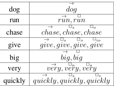
repre-sentations I am using is shown in Table 4.1.2

4.2.2

Semantic composition

My system incorporates semantic composition via two composition rules, one for

com-bining structures of different arity and the other for symmetric composition of structures

with the same arity. These rules incorporate insights of two empirically successful models,

lexical function and the simple additive approach, used as the default structure merging

strategy.

The first rule is function application, illustrated in Figure 4-1. Table 4.2 illustrates

1_{Matrices associated with term}_x_{are symbolized}2_𝑥_.

2_{To determine the number and ordering of matrices representing the word in the current syntactic context,}

(43)

dog

→

𝑑𝑜𝑔

run 𝑟𝑢𝑛,→ 𝑟𝑢𝑛2

chase → 𝑐ℎ𝑎𝑠𝑒, 2 𝑠 𝑐ℎ𝑎𝑠𝑒, 2 𝑜 𝑐ℎ𝑎𝑠𝑒 give →

𝑔𝑖𝑣𝑒,𝑔𝑖𝑣𝑒,2𝑠 𝑔𝑖𝑣𝑒,2𝑜 𝑔𝑖𝑣𝑒2𝑖𝑜

big

→

𝑏𝑖𝑔,𝑏𝑖𝑔2

very 𝑣𝑒𝑟𝑦,→ 𝑣𝑒𝑟𝑦,2𝑛 𝑣𝑒𝑟𝑦2𝑎

quickly

→

𝑞𝑢𝑖𝑐𝑘𝑙𝑦,𝑞𝑢𝑖𝑐𝑘𝑙𝑦,2𝑠 𝑞𝑢𝑖𝑐𝑘𝑙𝑦2𝑣

Table 4.1: Examples of word representations. Subscripts encode, just for mnemonic pur-poses, the constituent whose vector the matrix combines with: subject, object, indirect

object,noun,adjective,verb phrase.

⟨_→

𝑥 +2𝑛𝑥+𝑘×→𝑦 ,2𝑥1+2𝑦 , . . . ,1 2𝑥𝑛+2𝑦 , . . .𝑛 ⟩

⟨_→

𝑥 ,2𝑥 , . . . ,1 2𝑥 , . . . ,𝑛 2𝑛𝑥+𝑘⟩ ⟨_→

𝑦 ,2𝑦 , . . . ,1 2𝑦𝑛

⟩

Figure 4-1: Function application: If two syntactic sisters have different arity, treat the higher-arity sister as the functor. Compose by multiplying the last matrix in the functor tuple by the argument vector and summing the result to the functor vector. Unsaturated matrices are carried up to the composed node, summing across sisters if needed.

simple cases of function application. For transitive verbs semantic composition applies

iteratively as shown in the derivation of Figure 4-2. For ternary predicates such asgivein

a ditransitive construction, the first step in the derivation absorbs the innermost argument

by multiplying its vector by the thirdgivematrix, and then composition proceeds like for

transitives.

The second composition rule,symmetric compositionapplies when two syntactic sisters

are of the same arity (e.g., two vectors, or two vector-matrix pairs). Symmetric composition

simply sums the objects in the two tuples: vector with vector,𝑛-th matrix with𝑛-th matrix.

Symmetric composition is reserved for structures in which the function-argument

dis-tinction is problematic. Some candidates for such treatment are coordination and nominal

compounds, although I recognize that the headless analysis is not the only possible one

here. See two examples of Symmetric Composition application in Table 4.3.

(44)

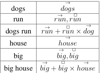
dogs

→

𝑑𝑜𝑔𝑠

run 𝑟𝑢𝑛,→ 𝑟𝑢𝑛2

dogs run 𝑟𝑢𝑛→ +𝑟𝑢𝑛2 ×

→ 𝑑𝑜𝑔 house → ℎ𝑜𝑢𝑠𝑒 big →

𝑏𝑖𝑔,𝑏𝑖𝑔2

big house

→

𝑏𝑖𝑔+𝑏𝑖𝑔2 ×

→

ℎ𝑜𝑢𝑠𝑒

Table 4.2: Examples of function application.

2𝑠

𝑐ℎ𝑎𝑠𝑒×𝑑𝑜𝑔𝑠→ +

→

𝑐ℎ𝑎𝑠𝑒+𝑐ℎ𝑎𝑠𝑒2𝑜 ×𝑐𝑎𝑡𝑠→

→

𝑑𝑜𝑔𝑠

⟨ _→

𝑐ℎ𝑎𝑠𝑒+𝑐ℎ𝑎𝑠𝑒2𝑜 ×𝑐𝑎𝑡𝑠,→ 𝑐ℎ𝑎𝑠𝑒2𝑠

⟩

⟨ _→

𝑐ℎ𝑎𝑠𝑒,𝑐ℎ𝑎𝑠𝑒,2𝑠 𝑐ℎ𝑎𝑠𝑒2𝑜

⟩ →

𝑐𝑎𝑡𝑠

Figure 4-2: Applying function application twice to derive the representation of a transitive sentence.

current PLF implementation treats most grammatical words, including conjunctions, as

“empty” elements, that do not project into semantics. This choice leads to some

interest-ing “serendipitous” treatments of various constructions. For example, since the copula is

empty, a sentence with a predicative adjective (cars are red) is treated in the same way

as a phrase with the same adjective in attributive position (red cars) – although the latter,

being a phrase and not a full sentence, will later be embedded as argument in a larger

con-struction. Similarly, leaving the relative pronoun empty makes cars that runidentical to

cars run, although, again, the former will be embedded in a larger construction later in the

sing:

→

𝑠𝑖𝑛𝑔,𝑠𝑖𝑛𝑔2 dance:

→

𝑑𝑎𝑛𝑐𝑒,𝑑𝑎𝑛𝑐𝑒2

sing and dance:

→

𝑠𝑖𝑛𝑔+

→

𝑑𝑎𝑛𝑐𝑒,𝑠𝑖𝑛𝑔2 +𝑑𝑎𝑛𝑐𝑒2

rice: → 𝑟𝑖𝑐𝑒 cake: → 𝑐𝑎𝑘𝑒 rice cake → 𝑟𝑖𝑐𝑒+ → 𝑐𝑎𝑘𝑒

(45)

derivation.

I conclude my brief exposition of PLF with an alternative intuition for it: the PLF model

is also a more sophisticated version of the additive approach, where argument words are

adapted by matrices that encode the relation to their functors before the sentence vector is

derived by summing.

4.2.3

Satisfying the desiderata

Let us now outline how PLF addresses the shortcomings of LF listed in Section 4.1.1. First,

all issues caused by representation size disappear. An n-ary predicate is no longer encoded

as an n+1-way tensor; instead I have a sequence of n matrices. The representation size

grows linearly, not exponentially, for higher semantic types, allowing for simpler and more

efficient parameter estimation, storage, and computation.

As a consequence of this architecture, we no longer need to perform the complicated

step-by-step estimation for elements of higher arity. Indeed, one can estimate each matrix

of a complex representation individually using the simple method of Baroni and Zamparelli

(2010). For instance, for transitive verbs I estimate the verb-subject combination matrix

from subject and verb-subject vectors, the verb-object combination matrix from object and

verb-object vectors. I expect a reasonably large corpus to feature many occurrences of a

verb with a variety of subjects and a variety of objects (but not necessarily a variety of

subjects with each of the objects as required by Grefenstette et al.’s training), allowing us

to avoid the data sparseness issue.

The semantic representations I propose include a semantic vector for constituents of any

semantic type, thus enabling semantic comparison for words of different parts of speech

(the case ofdemolitionvs.demolish).

Finally, the fact that I represent the predicate interaction with each of its arguments in

a separate matrix allows for a natural and intuitive treatment of argument alternations. For

instance, as shown in Table 4.4, one can distinguish the transitive and intransitive usages of

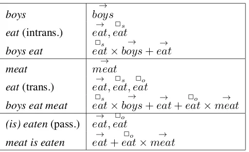
the verbto eatby the presence of the object-oriented matrix of the verb while keeping the

(46)

boys

→

𝑏𝑜𝑦𝑠

eat(intrans.) 𝑒𝑎𝑡,→ 𝑒𝑎𝑡2𝑠

boys eat 𝑒𝑎𝑡2𝑠 ×

→

𝑏𝑜𝑦𝑠+𝑒𝑎𝑡→

meat 𝑚𝑒𝑎𝑡→

eat(trans.)

→

𝑒𝑎𝑡,𝑒𝑎𝑡,2𝑠 𝑒𝑎𝑡2𝑜

boys eat meat 𝑒𝑎𝑡2𝑠 ×𝑏𝑜𝑦𝑠→ +𝑒𝑎𝑡→ +𝑒𝑎𝑡2𝑜 ×𝑚𝑒𝑎𝑡→

(is) eaten(pass.)

→

𝑒𝑎𝑡,𝑒𝑎𝑡2𝑜

meat is eaten 𝑒𝑎𝑡→ +𝑒𝑎𝑡2𝑜 ×𝑚𝑒𝑎𝑡→

Table 4.4: The verb to eat associated to different sets of matrices in different syntactic contexts.

verb only, which will be multiplied by the syntactic subject vector, capturing the similarity

betIeneat meatandmeat is eaten.

So keeping the verb’s interaction with subject and object encoded in distinct matrices

not only solves the issues of representation size for arbitrary semantic types, but also

pro-vides a sensible built-in strategy for handling a word’s occurrence in multiple constructions.

Indeed, if we encounter a verb used intransitively which was only attested as transitive in

the training corpus, we can simply omit the object matrix to obtain a type-appropriate

rep-resentation. On the other hand, if the verb occurs with more arguments than usual in testing

materials, we can add a default diagonal identity matrix to its representation, signaling

ag-nosticism about how the verb relates to the unexpected argument. This flexibility makes my

model suitable to compute vector representations of sentences without stumbling at unseen

syntactic usages of words.

To summarize, PLF is an extension of the lexical function model that inherits its strengths

and overcomes its weaknesses. I still employ a linguistically-motivated notion of semantic

composition as function application and use distinct kinds of representations for

differ-ent semantic types. At the same time, I avoid high order tensor represdiffer-entations, produce

semantic vectors for all syntactic constituents, and allow for an elegant and transparent

correspondence between different syntactic usages of a lexeme, such as the transitive, the

intransitive, and the passive usages of the verbto eat. Last but not least, my implementation

(47)

of arbitrary size, including those containing novel syntactic configurations.

4.3

Evaluation

4.3.1

Evaluation materials

Here I want to evaluate the models on sentence level, instead of phrase level like in

chap-ter 3. Therefore, I consider 5 different benchmarks that focus on different aspects of

sentence-level semantic composition. The first data set, created by Edward Grefenstette

and Mehrnoosh Sadrzadeh and introduced in Kartsaklis e

Sentential Representations in Distributional Semantics