Quantifying the impact of ocean acidification on our future climate

www.biogeosciences.net/11/3965/2014/ doi:10.5194/bg-11-3965-2014

© Author(s) 2014. CC Attribution 3.0 License.

Quantifying the impact of ocean acidification on our future climate

R. J. Matear and A. Lenton

Centre for Australian Weather and Climate Research (CAWCR). A partnership between CSIRO and the Bureau of

Meteorology; CSIRO Marine and Atmospheric Research, CSIRO Marine Laboratories, GPO Box 1538, Hobart, Tasmania, Australia

Correspondence to: R. J. Matear ([email protected])

Received: 21 September 2013 – Published in Biogeosciences Discuss.: 12 November 2013 Revised: 23 May 2014 – Accepted: 6 June 2014 – Published: 30 July 2014

Abstract. Ocean acidification (OA) is the consequence of rising atmospheric CO2 levels, and it is occurring in con-junction with global warming. Observational studies show that OA will impact ocean biogeochemical cycles. Here, we use an Earth system model under the RCP8.5 emission sce-nario to evaluate and quantify the first-order impacts of OA on marine biogeochemical cycles, and its potential feedback on our future climate. We find that OA impacts have only a small impact on the future atmospheric CO2 (less than 45 ppm) and global warming (less than a 0.25 K) by 2100. While the climate change feedbacks are small, OA impacts may significantly alter the distribution of biological produc-tion and remineralisaproduc-tion, which would alter the dissolved oxygen distribution in the ocean interior. Our results demon-strate that the consequences of OA will not be through its impact on climate change, but on how it impacts the flow of energy in marine ecosystems, which may significantly im-pact their productivity, composition and diversity.

1 Introduction

The oceans have taken up approximately a third of the to-tal fossil fuel CO2emitted to the atmosphere since the onset of industrialisation (140±25 PgC, (Khatiwala et al., 2009)). This uptake has slowed the rate of global warming, but has led to detectable changes in the ocean chemistry (e.g. Doney et al., 2009). As the CO2enters the ocean, primarily through sea–air fluxes, it reacts with the seawater and reduces the carbonate ion concentration and pH, collectively known as ocean acidification (OA). This uptake of anthropogenic CO2 has reduced the pH of the modern ocean surface waters by 0.1 units or hydrogen ion concentration ([H+]) by 30 % since

preindustrial times (Caldeira, 2005). By the end of this cen-tury, under the higher emission scenarios, the projected [H+] change since preindustrial times maybe greater than 100 % (Orr et al., 2005).

OA has the potential to affect the major biogeochemical (BGC) cycles in the ocean (Gehlen et al., 2011), with poten-tially significant consequences for our future climate (Matear et al., 2010). In assessing the potential OA impacts on BGC cycles and climate, it is important to recognise that ocean acidification impacts do not occur in isolation, but they are associated with global warming, which may modulate their impacts (e.g. Brewer and Peltzer, 2009). Therefore, assess-ing the future impacts of OA requires an Earth System Model (ESM) that considers the interactive effects of global warm-ing and OA on BGC cyclwarm-ing (Tagliabue et al., 2011). The goal of this study is to use an ESM to evaluate and quan-tify the first-order impacts and climate feedbacks of OA. To do this, we first review the potential for ocean acidification to alter the major BGC cycles. We then use our ESM to as-sess how these modulations of the BGC by OA alter the pro-jected climate in the current century. From our simulations, we then discuss how the OA-modulated BGC changes affect the ocean environment. Finally, we conclude with a discus-sion of OA impacts on BGC cycling and climate that require further investigation.

2 Potential impacts of ocean acidification on BGC cycles

feedback) or reduce (negative feedback) global warming due to rising or respectively decreasing greenhouse gases. For this study, we primarily focus on marine BGC processes that are impacted by OA and global warming, which can alter oceanic uptake of carbon.

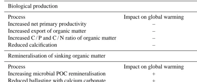
To aid the discussion of the potential impacts of OA on BGC cycles, we separate the impacts into processes that (1) alter biological production in the photic zone; and (2) alter the remineralisation of sinking particulate organic and inor-ganic carbon in the ocean interior. These processes are sum-marised in Table 1, with an indication of the sign the impact has on global warming based on published studies.

2.1 Biological production

The rising CO2levels in the upper ocean has the potential to affect biological production in several ways:

1. Increase net primary productivity by making photosyn-thesis more efficient (Rost et al., 2008). Experimental studies have also shown an increase in particulate or-ganic carbon (POC) production in response to increased levels of CO2(e.g. Zondervan et al., 2002).

2. Alter the stoichiometric nutrient to carbon ratio of the exported particulate organic matter, which enables ocean biology to partially overcome nutrient control on carbon production and export. Mesocosm experiments with natural plankton communities have reported an in-creased C / N ratio of particulate organic matter under elevated CO2 (Riebesell et al., 2007; Bellerby et al., 2008). In these experiments, the C / N ratio increased from 6.0 at 350 µatm to 8.0 at about 1050 µatm. An in-crease in the C / N ratio of the export POC with a fixed C / O ratio would result in increased carbon storage and increased oxygen consumption in the ocean (Oschlies et al., 2008).

3. Impact the ability of organisms to calcify (Fabry et al., 2008). This is anticipated to reduce the production of calcium carbonate. Due to the nature of the carbon-ate chemistry, reduced calcium carboncarbon-ate production allows the upper ocean to increase its carbon uptake (Raven, 2005; Heinze, 2004; Hutchins, 2011).

All three of these affects would increase the storage of car-bon in the ocean and provide a negative feedback to climate warming.

2.2 Remineralisation of particulate material

Most of the exported POC is remineralised in the upper 1000 m, but ≈10 % escapes to the deep ocean, where it is remineralised or buried in sediments, and sequestered from the atmosphere on millennium timescales (Trull et al., 2001). Analysis of particulate inorganic carbon (PIC) and POC fluxes at water depths greater than 1000 m suggests a close

association between these fluxes (Armstrong et al., 2002). The ratio of PIC production to POC is called the rain ratio (e.g. Archer et al., 2000). OA has the potential to impact the remineralisation of sinking particulate material in the follow-ing ways:

1. Dissolution of CaCO3 is an abiotic process driven by thermodynamics, and the rate of dissolution is related to the saturation state of the ocean (Orr et al., 2005). Chemical dissolution can occur when the saturation state of CaCO3falls below 1 (or below the lysocline). As the lysocline moves toward the surface with ocean acidification, increased dissolution of CaCO3sediments and sinking particles will increase the alkalinity in the ocean (Ridgwell et al., 2009). This potentially increases the supply of alkalinity to the upper ocean (increasing CO2uptake), which acts as a negative climate feedback. 2. (Armstrong et al., 2002) proposed that CaCO3acts as a carrier for transporting POC to the deep ocean by bal-lasting the POC, thereby increasing its sinking speed. It is also hypothesised that the association between CaCO3and POC might protect the latter from bacte-rial degradation (Armstrong et al., 2002). If deep-water POC fluxes are controlled by CaCO3, then a decrease in the CaCO3production would result in a decreased POC transport to the deep ocean. Consequently, POC would remineralise at shallower depths and therefore the net efficiency of the biological pump would decrease, re-sulting in a positive climate feedback.

3. The remineralisation length scale of POC is depen-dent on microbial activity. It has been hypothesised that ocean acidification may increase the rate of microbial activity (Weinbauer et al., 2011), leading to more rapid remineralisation of sinking POC, which would result in less carbon sequestration, and a positive climate feed-back. A warming ocean may further accelerate micro-bial activity (Rivkin, 2001) and cause more rapid rem-ineralisation of sinking POC.

In summary, changing the strength of the biological pump can have either a positive or negative feedback on climate warming.

3 Earth system model and simulations 3.1 Earth system model

Table 1. Potential ocean acidification impacts on BGC cycles. A positive value in the Impact on global warming column signifies the process

causes greater warming (positive feedback).

Biological production

Process Impact on global warming

Increased net primary productivity – Increased export of organic matter – Increased C / P and C / N ratio of organic matter –

Reduced calcification –

Remineralisation of sinking organic matter

Process Impact on global warming

Increasing microbial POC remineralisation + Reduced ballasting with calcium carbonate +

2003; Duteil et al., 2012). The details of the ocean biogeo-chemical model are summarised in the Appendix.

The atmosphere model has a horizontal resolution of 5.6◦C by 3.2◦C, and 18 vertical layers. The land carbon model has the same horizontal resolution as the atmosphere. The ocean model has a resolution of 2.8◦C by 1.6◦C, and 21 vertical levels. Mk3L simulates the historical climate well, as compared to the models used for earlier IPCC assess-ments (Phipps et al., 2011; Pitman et al., 2011). Furthermore, the simulated response of the land carbon cycle to increas-ing atmospheric CO2and warming are consistent with those from the Coupled Model Intercomparison Project Phase 5 (CMIP5) (Zhang et al., 2014). The ocean biogeochemical model was shown to realistically simulate the global ocean carbon cycle (Duteil et al., 2012). Previous studies with this ocean biogeochemical model have shown to realistically sim-ulate anthropogenic carbon and CFC uptake by the ocean (Matsumoto et al., 2004). We referred to the ocean BGC for-mulation used in these previous studies as our standard BGC formulation, which is then modified to incorporate OA im-pacts.

The land model (CABLE) with CASA-CNP simulates the temporal evolution of heat, water and momentum fluxes at the surface, as well as the biogeochemical cycles of car-bon, nitrogen and phosphorus in plants and soils. For this study, we used the spatially explicit estimates of nitrogen de-position for 1990 (Dentener, 2006). The simulated (Zhang et al., 2014) geographic variations of nutrient limitations, major biogeochemical fluxes and pools on the land under the present climate conditions are consistent with published studies (Wang et al., 2010; Hedin, 2004).

3.2 Model simulations

The ESM was spun up under preindustrial atmospheric CO2 (1850: 284.7 ppm) until the simulated climate became stable. Stability was defined as the linear trend of global mean sur-face temperature over the last 400 years of the spin-up being less than 0.015 K per century.

For the historical period (1850–2005), the ESM was run using the historical atmospheric CO2concentrations as pre-scribed by the CMIP5 simulation protocol. For the historical period a reference simulation (REF) was performed where at-mospheric CO2affects both the radiative properties of the at-mosphere and the carbon cycle (Table 2) (Zhang et al., 2014). For the future, we used the RCP8.5 emissions scenario as provided by the CMIP5 (http://cmip-pcmdi.llnl.gov/cmip5/), and let our ESM, which has full carbon–climate interac-tions, determine the future atmospheric CO2concentrations (Zhang et al., 2014). The RCP8.5 scenario is the highest CO2 emissions scenario used in the IPCC’s Fifth Assess-ment Report, and in this scenario radiative forcing increases to 8.5 W m−2_{by 2100. For comparison, we also completed a} standard CMIP5 simulation where RCP8.5 atmospheric CO2 concentrations were used rather than letting our ESM deter-mine the future CO2concentrations from the emission sce-nario (we called this simulation RCP8.5). As discussed by (Zhang et al., 2014), using RCP8.5 emissions rather than concentrations resulted in a slightly warmer world (0.25 K) by 2100 because of reduced land carbon uptake due to nutri-ent limitation. In all our simulations the vegetation scenario used by (Lawrence et al., 2013) remained unchanged over the simulation period following the CMIP5 experimental de-sign. Note that the CO2emissions from land use change were not included in our simulation, but are implicitly taken into account in the the RCP8.5 emission scenario. We also ne-glected changes in anthropogenic N deposition over the sim-ulation period, because of the large uncertainty in the future deposition rate and the small impact it has on net land carbon uptake (Zaehle et al., 2010).

3.3 Ocean acidification impacts on BGC

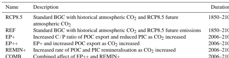
Table 2. Summary of the ocean BGC experiments presented in this study. In all simulations, both the climate and the carbon components

experience the impact of rising atmospheric CO2. The RCP8.5 simulation uses the prescribed atmospheric CO2as provided by the CMIP5 for this scenario, while the others scenarios use the RCP8.5 emissions and the ESM determines the CO2concentration. In the REF and RCP8.5 simulations, the formulation of the ocean BGC is not impacted by OA, while in the other simulations selected processes are modified to address the potential OA impacts. The REF simulation starts in 1850 using historical atmospheric CO2(identical to RCP8.5) and switches to the RCP8.5 future emissions scenario at the start of 2006. The four other simulations (EP+, EP++, REMIN+ and COMB) start from the REF simulation at the end of 2005 and go until 2100 using the RCP8.5 future emissions. Please refer to the text for a description of how the BGC cycle is modified in the EP+, EP++, REMIN+ and COMB simulations.

Name Description Duration

RCP8.5 Standard BGC with historical atmospheric CO2and RCP8.5 future 1850–2100 atmospheric CO2

REF Standard BGC with historical atmospheric CO2and RCP8.5 future emissions 1850–2100 EP+ Increased C / P ratio of POC export and reduced PIC as CO2increased 2006–2100 EP++ EP+ and increased POC export as CO₂increased 2006–2100 REMIN+ Increased rate of POC and PIC remineralisation as CO2increased 2006–2100

COMB Combined affect of EP++ and REMIN+ 2006–2100

first-order assessment of the OA impacts discussed in Sect. 2 on the future climate.

The reference simulation (REF), refers to the standard BGC formulation with no OA impacts. With this ocean BGC formulation, the ESM simulates the years 1850 to 2100 us-ing historical atmospheric CO2 for 1850 to 2005 and then the RCP8.5 emissions until the year 2100. All of the remain-ing experiments to be discussed were started from the year 2006 and use the same RCP8.5 emissions as the REF sim-ulation. In the REF simulation, the ratio of exported PIC to POC (ro) was kept constant, which implies the simula-tion includes a temperature effect on PIC producsimula-tion because the PIC production would increases as a warming ocean in-creases POC production (Pinsonneault et al., 2012; Schmit-tner et al., 2008).

The first OA simulation (EP+) considers the impact of ris-ing CO2 on the C / P ratio of the exported POC. The C / P changes are based on (Oschlies et al., 2008), while the C / O of POC and the PIC export remain unchanged. The modi-fied POC export (QC_POC) is given by the following equations, where CO2is the atmospheric CO2 concentration,QP_POC is the phosphate uptake in the photic zone and1zis the depth of the photic zone.

QPOC=106QPPOCFo1z (1)

Fo=1+(CO2−380)·2.3/700/6.6, for CO2>380 (2) At the start of the experiment (2006), the atmospheric CO2 equals 380 ppm and the scaling factor (Fo) is equal to 1 (C / N = 6.6), which is the value used in the REF experiment. At the end of the experiment (2100), the atmospheric CO2 equals 1010 ppm and the scaling factor (Fo) 1026 (C / N = 1.32).

In the second OA experiment (EP++), in addition to the EP+ modification, the export of POC is prescribed to increase as atmospheric CO2levels rise, reflecting the enhanced pro-duction due to enhanced photosynthesis with increased CO2. In addition, the PIC export (QC_PIC) is prescribed to decline

as calcification decreases with rising CO2 (Ridgwell et al., 2009). To achieve this we increase the POC export scaling factor (SnppEq. A6, see Appendix), which increases POC ex-port and reduces the rain ratio between PIC and POC exex-port (r) with atmospheric CO2as follows:

Snpp=Snppo [4.5·(CO2/380)−3.5] (3)

QPIC=r106QPPOC1z (4)

r=ro·1/(9.5·CO2/380−8.5), (5) where S_nppo and ro are the values used in the REF and the RCP8.5 experiments. At an atmospheric CO2 level of 1140 ppm (the approximate value in our REF simulation at 2100) the POC export scaling factor is 10 times and the rain ratio is 5 % of the REF experiment. Note that while the scal-ing factor was increased by 10 times, the actual increase in export of POC was still constrained by the availability of phosphate and light, which dramatically reduces the increase in POC export in this experiment.

In the third OA simulation (REMIN+), the standard BGC formulation was used but both the remineralisation of POC and the dissolution of PIC are enhanced. The increased POC remineralisation reflects an increasing rate of microbial ac-tivity with OA. The increased PIC dissolution reflects the im-pact of OA on the chemical dissolution of PIC. In the previ-ously discussed experiments, POC and PIC have prescribed depth profiles (see A18 and A19 in Appendix), which are now modified by the atmospheric CO2as follows to give an upper bound estimate of the potential impact of increased POC remineralisation and increased PIC dissolution on car-bon storage in the ocean.

experiment, where REMINo_POC= −0.9 and REMINo_PIC = 3500 in the REF simulation (see equations A18 and A19). With an atmospheric CO2 level of 1000 ppm, the depth of remineralisation declines by 2.25 from the REF experiment. For POC, this means the POC that sinks below 200 m de-clines from 54 % in REF simulation to 25 %. For PIC, the PIC sinking below 1000 m reduces from 75 % in REF simu-lation to 37 %.

These BGC changes are an idealised representation of the OA impact on the ocean BGC cycle. They were deliberately chosen to provide extreme perturbations to the BGC cycle and to test the potential for these impacts to have a significant consequence on the future projected climate.

4 Results and discussion

We will first present and discuss the REF simulation by as-sessing its present-day ocean state and its projected response to the RCP8.5 emission scenario. Then, we will project and discuss how OA impacts the ocean BGC cycle, and how this in turn impacts the future atmospheric CO2 concentration and climate.

4.1 Historical period

For the historical period, the simulated global surface warm-ing generally agrees with the observed warmwarm-ing. The ob-served global surface temperature increase between 1850– 1899 and 2001–2005 is 0.76±0.19 K (Trenberth et al., 2007) compared to the simulated increase of 0.57±0.07 K (Zhang et al., 2014). The observed land surface temperature increase from 1850–1899 to 2001–2005 is 1.0±0.25 K (Brohan et al., 2006) compared to a simulated increase of 0.75±0.06 K (Zhang et al., 2014).

(Zhang et al., 2014) assessed the simulated anthropogenic CO2 uptake by the land and ocean, and showed that over the historical period the model realistically reflected the ob-served estimates. From 1850 to 2005, the total carbon ac-cumulated in the land biosphere is 85 Pg C, which is within the estimated land carbon uptake of 135±85 Pg C calcu-lated from the estimated rates of ocean carbon uptake and atmospheric growth (Zhang et al., 2014). The simulated carbon accumulated in the ocean (118 Pg C) agrees with the estimated anthropogenic carbon storage in the ocean of 135±25 Pg C (Khatiwala et al., 2009). (Zhang et al., 2014) also showed that simulated land and ocean carbon uptakes are consistent with the latest synthesis for the period 1960 to 2005 (Canadell et al., 2007).

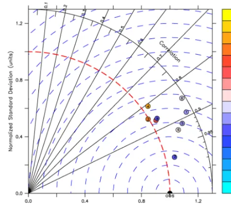
To assess the realism of the ocean carbon simulation we compare (1) dissolved oxygen at 500 m; (2) surface arago-nite saturation state (3) aragoarago-nite lysocline depth; (4) the sur-face phosphate; (5) global alkalinity; (6) global preindustrial dissolved inorganic carbon; (7) global phosphate; (8) global oxygen; and (9) global apparent oxygen utilisation (AOU)

Figure 1. Taylor diagram of the comparison of the simulated fields

with the observations for surface phosphate (1), dissolved oxygen at 500 m (2), surface aragonite saturation state (3), lysocline depth (4), and the three-dimensional fields of alkalinity (5), preindustrial dissolved inorganic carbon (6), dissolved oxygen (7), phosphate (8) and apparent oxygen utilisation (9). The observations are based on (Key et al., 2004) and (Boyer et al., 2009); the REF 1995 simulated fields are used for the comparison except for preindustrial inorganic carbon, which comes from the REF simulation in 1850. The colour bar gives the bias in the simulated fields normalised by the standard deviation in the observed fields. The plotted data are summarised in Table 3.

with the observations (Key et al., 2004; Boyer et al., 2009) using a Taylor (2001) (Fig. 1). We use the Taylor diagram to provide a quantitative assessment of the simulated fields, and the statistics shown in the Taylor diagram are summarised in Table 3. For visual comparisons of the simulation with observations see the Appendix; where, zonally averaged sec-tions of alkalinity and preindustrial dissolved organic carbon (Fig. A1), along with global averaged profiles of alkalinity, preindustrial dissolved organic carbon, phosphate, oxygen and apparent oxygen utilisation (Fig. A2) are shown.

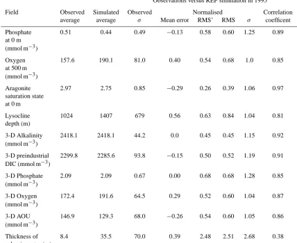
Table 3. Summary statistics of the comparison of the REF simulated fields with the observations shown in Fig. 1. All simulated fields are

based on the REF 1995 values except for preindustrial dissolved inorganic carbon which comes from the REF 1850 simulation fields.

Observations versus REF simulation in 1995

Field Observed Simulated Observed Normalised Correlation average average σ Mean error RMS’ RMS σ coefficent

Phosphate 0.51 0.44 0.49 −0.13 0.58 0.60 1.25 0.89

at 0 m (mmol m−3)

Oxygen 157.6 190.1 81.0 0.40 0.54 0.68 1.0 0.85

at 500 m (mmol m−3)

Aragonite 2.97 2.75 0.85 −0.29 0.26 0.39 1.06 0.97

saturation state at 0 m

Lysocline 1024 1407 679 0.56 0.63 0.84 1.04 0.81

depth (m)

3-D Alkalinity 2418.1 2418.1 44.2 0.0 0.45 0.45 1.15 0.92 (mmol m−3)

3-D preindustrial 2299.8 2285.6 93.8 −0.15 0.50 0.52 1.19 0.91 DIC (mmol m−3)

3-D Phosphate 2.09 2.09 0.67 0.00 0.68 0.68 1.28 0.85 (mmol m−3)

3-D Oxygen 172.4 191.6 64.5 0.29 0.52 0.60 1.04 0.87 (mmol m−3)

3-D AOU 146.9 129.3 68.0 −0.26 0.54 0.60 1.05 0.86

(mmol m−3)

Thickness of 8.4 35.5 70.0 0.39 2.48 2.51 2.68 0.38

suboxic water (m)

less than observed (Table 3). While the simulated three-dimensional AOU concentrations are highly correlated with the observations (r=0.86), (Duteil et al., 2013) showed that this model has a mid-depth AOU maximum in the Pacific that is too small. This implies that the simulation is either over-ventilating the Pacific intermediate waters, or underes-timating the remineralisation of POC in the ocean interior.

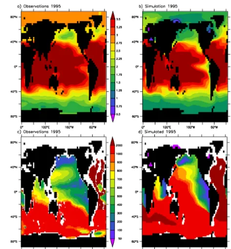
Fig. 2.Annual mean for the year 1995 comparison of the observed and simulated fields for a-b) thickness of suboxic layer (m), and c-d ) surface phosphate concentration (mmol/m3_{). The suboxic waters are} characterised by oxygen concentrations less than 5mmol/m3_{). The observed fields are based on Boyer} et al. (2009).

34

Figure 2. Annual mean for the year 1995 comparison of the

ob-served and simulated fields for (a, b) thickness of suboxic layer (m), and (c, d) surface phosphate concentration (mmol m−3). The suboxic waters are characterised by oxygen concentrations less than 5 mmol m−3). The observed aragonite saturation was calculated us-ing Key et al. (2004) and Boyer et al. (2009) gridded datasets.

For surface aragonite saturation state, the REF simulation was highly correlated with the aragonite saturation state cal-culated from the observations (Key et al., 2004), with the simulation slightly underestimating the average saturation state (Fig. 3 and Table 3).

In the ocean interior, the REF simulation has a similar pat-tern of the aragonite lysocline to that observed. In general, the simulated lysocline depth is a little deeper than observed, except in the western Pacific, where the simulated values are several hundred metres too deep (Fig. 3 and Table 3). For the simulated three-dimensional alkalinity and preindustrial dissolved inorganic carbon concentrations, the REF simula-tion is highly correlated with the observasimula-tions (0.92 and 0.91, respectively), whereas spatial variability slightly exceeds the observations with a mean dissolved inorganic carbon concen-tration that is 15 mmol m−3_{less than observed (Table 3). The} simulated global averaged dissolved inorganic carbon con-centration that is less than observed is consistent with the underestimation of POC remineralisation in the ocean inte-rior.

To assess the ocean circulation of the REF simulation, we use the analysis of (Matsumoto et al., 2004). They show the CSIRO model in their study, which is nearly identical to the REF simulation presented here, correctly ventilated the ocean on decadal and centennial timescales based on

simu-Fig. 3.Annual mean for the year 1995 comparison of the observed and simulated fields for a-b) surface aragonite saturation state c-d ) aragonite lysocline depth (m) The observations for aragonite saturation are calculated from Key et al. (2004).

35

Figure 3. Annual mean for the year 1995 comparison of the

ob-served and simulated fields for (a, b) surface aragonite saturation state (c, d) aragonite lysocline depth (m); and thickness of the sub-oxic layer (m). The observations for aragonite saturation are calcu-lated from (Key et al., 2004).

lated CFC-11, natural radiocarbon and anthropogenic carbon concentrations.

In summary, the REF simulation generally reflects the present-day ocean state (correlation coefficient with observa-tions greater than 0.8). However, the important discrepancies with the observations are that the suboxic layer is too thick, the lysocline in the Western Pacific subtropical and equato-rial water is too deep, and the remineralisation of POC in the ocean interior is less than observed. These model biases are considered when assessing the projected regional changes as-sociated with OA.

4.2 Future OA impacts on ocean BGC 4.2.1 Carbon climate feedbacks

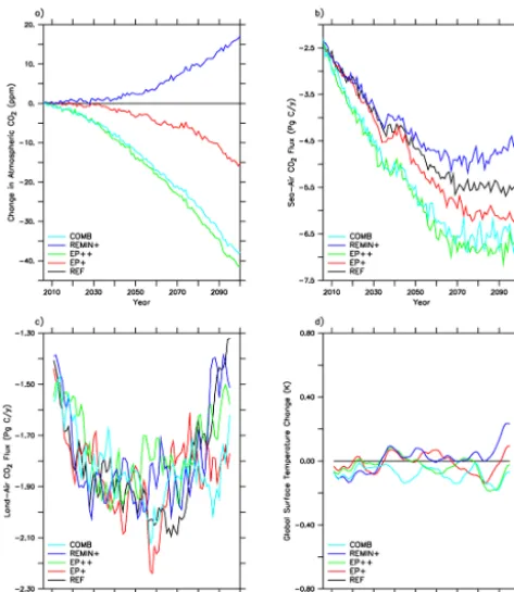
Figure 4. (a) Change in atmospheric CO2(ppm) for the future pe-riod relative to the REF simulation for the various OA experiments (see Table 2 for a description of the experiments). (b) Simulated global ocean carbon uptake for the different OA experiments. (c) Simulated 10-year running mean of the land carbon uptake by the different OA experiments. (d) Simulated 10-year running mean of the change in global surface temperature relative to the REF simu-lation for the various OA experiments.

difference between EP++ and REMIN+ simulations because the combination of larger export with shallower recycling of POC is more efficient at storing carbon in the ocean than when the two changes are considered individually. For the global climate, the OA impacts of these small atmospheric CO2changes leads to global surface temperature deviations of less than 0.25 K (Fig. 4).

4.2.2 Changes in BGC fields

While the OA impacts on the ocean carbon storage and cli-mate by the end of this century are small, we investigate whether the BGC fields in the ocean are significantly altered by OA. Key ocean BGC fields that have been shown to be im-pacted by global warming and OA are aragonite saturation state, lysocline depth, export production, dissolved oxygen and volume of suboxic water. Here, we focus on how the OA impacts each of these fields relative to the REF simulation.

Figure 5. Annual mean surface aragonite saturation state during the

2090–2100 period for (a) REF; (b) EP+; (c) EP++; (d) REMIN+; and (e) COMB simulations.

4.2.3 Aragonite saturation state

For the surface aragonite saturation state, there are only sub-tle differences among the simulations (Fig. 5). As expected, all simulations show a dramatic reduction in the surface arag-onite saturation state by 2100, with the surface water pole-ward of approximately 40◦S and 40◦N being undersaturated with respect to aragonite (Fig. 5). By 2100, the REF simu-lation has an atmospheric CO2 value of 1026 ppm. At low latitudes, by 2100 the maximum aragonite saturation state from all simulations is less than 2.75, which is a saturation state level in which historically no living corals are observed (Guinotte et al., 2003). In all simulations, the upwelling re-gion of the eastern Equatorial Pacific shows a minimum in the tropical aragonite saturation state.

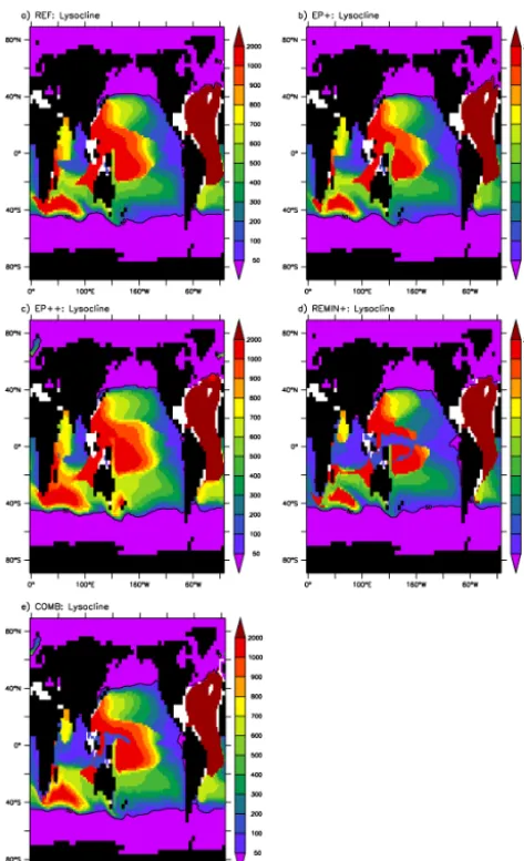
Figure 6. Annual mean depth of the aragonite lysocline (m)

dur-ing the 2090–2100 period for: (a) REF; (b) EP+; (c) EP++; (d) REMIN+; and (e) COMB simulations.

simulations, the eastern tropical and subtropical Pacific lyso-cline is less than 100 m deep. Similarly, all simulations show lysocline depths of less than 100 m in the Indian Ocean. It is only in the equatorial western Pacific that the lysocline depths remain greater than 1000 m by 2100. Note that this is the region where the REF simulation overestimated the lysocline depth by several hundred metres, and in the OA experiments this region retains its resilience to change. This probably reflects a bias in the model, and we anticipate that the region would show much greater shoaling by the end of the century consistent with (Bopp et al., 2013).

Overall, the OA impacts only make subtle changes to the overall dramatic reduction in surface aragonite saturation state and lysocline depth projected with the RCP8.5 emis-sion scenario.

Figure 7. (a) Projected global export of POC from the upper 100 m

of the ocean. (b) Projected global export of PIC from the upper 100 m of the ocean.

4.2.4 Export production

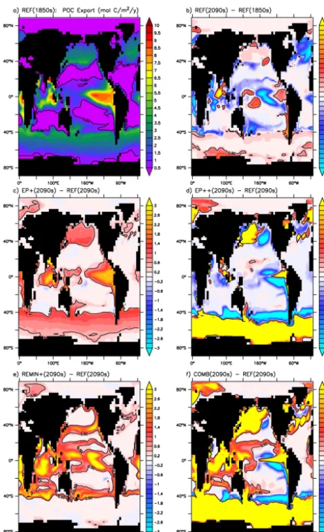
For the export of POC from the upper ocean, in the REF simulation shows a small global reduction (Fig. 7), which is mostly confined to the equatorial Pacific, Indian and North Atlantic oceans (Fig. 8) associated with increased upper ocean stratification that occurs in climate change projections (e.g. Matear and Hirst, 1999). The export of PIC from the up-per ocean is also shown in Fig. 7, with all exup-periments show-ing a decline global export in the future except for REMIN+. In the REMIN+ simulation, the increase in POC export is associated with an increase in PIC export because the rain ratio was held constant. Interestingly, the different OA ex-periments show large regional differences in export produc-tion (Fig. 8), with EP++ and COMB substantially increasing export production in the Southern Ocean. However, for the global integrated value, all OA impacts cause an increase in POC export production, with the greatest increase occurring in the COMB projection.

The large range in the export production response to the different OA experiments is consistent with previous studies (e.g. Tagliabue et al., 2011). The simulations reveal that OA impacts on export production are much greater than their im-pacts on climate change. Such behaviour demonstrates that the consequence of OA will not be through its impact on cli-mate change, but on how it impacts the flow of energy in marine ecosystems. These changes may have significant im-pacts on marine ecosystems and their productivity, biodiver-sity, and our future ability to exploit them as a food resource. 4.2.5 Dissolved oxygen

Figure 8. Export production (mol C m−2yr−1) from the (a) REF in 1850; (b) the change in 2090–99 mean for REF relative to (a). For the 2090–2099 mean, the change relative to REF for (c) EP+; (d) EP++; (e) REMIN+; (f) COMB simulations.

to alter dissolved oxygen levels in the ocean. With climate change, the REF simulation shows a decline in the mid-water dissolved oxygen levels in the North Pacific, equatorial Pa-cific and Southern oceans (Fig. 9).

The oceanic oxygen levels are expected to decline under global warming (e.g. Matear et al., 2000; Bopp et al., 2002), because surface warming lowers the sea surface oxygen con-centrations, enhances stratification, reduces ventilation of the thermocline, and reduces thermohaline circulation, which all tend to decrease the supply of oxygen to the ocean inte-rior. The reduced oxygen supply to the ocean interior is also linked to increased residence time of water at depth, thereby enhancing biological oxygen consumption in the ocean inte-rior.

Figure 9. Dissolved oxygen (mmol m−3) at 500 m for (a) REF in 1850; (b) the change in 2090–2099 mean for REF relative to (a). For the 2090–99 mean, the change relative to REF for (c) EP+; (d) EP++; (e) REMIN+; (f) COMB simulations.

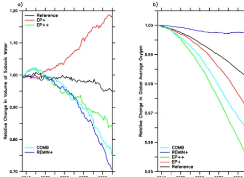
Figure 10. (a) The ratio of the simulated change in the volume of

suboxic water to the simulated present-day (2006) value. (b) The ratio of the simulated change in the global ocean inventory of dis-solved oxygen to the simulated 2006 value.

the ocean displays a complex regional pattern with both pos-itive and negative trends reflecting the complex interactions between changes in circulation, biological production, bio-logical remineralisation, and temperature.

The inclusion of OA impacts that could either increase POC export from the upper ocean (Fig. 7) and/or reduce its depth of remineralisation may substantially decrease oxygen levels in the ocean interior. For the total oxygen inventory in the ocean, the simulations reveal that increased POC ex-port causes a decline in oxygen, while the shoaling of POC remineralisation has little impact (Fig. 10b).

The EP+ simulation showed a 17 % increase in the thick-ness in the suboxic water by 2100 (Fig. 10a). Similar simu-lations where the C / N ratio of exported POC matter is in-creased with OA project reduced dissolved oxygen levels in the ocean and a comparable increase in the volume of sub-oxic water to the EP+ projection (Oschlies et al., 2008; Tagli-abue et al., 2011).

(Oschlies et al., 2008) shows the volume of suboxic wa-ter is very sensitive to small changes in the remineralisation of POC in the ocean interior. Our simulations confirm this result, but also show the volume of suboxic water is sensi-tive to the location where OA increases POC export. With the shoaling of POC remineralisation (REMIN+) there is a reduction in the volume of suboxic water. By confining POC remineralisation to the upper ocean, the equatorial Pacific has less suboxic water, because this water is now more influenced by air–sea gas exchange, there is a global decline in the vol-ume of suboxic water (Fig. 10). Similarly, the EP++ simu-lation with increased export production shows the greatest decline in total oxygen inventory (Fig. 10b), but a decline in the volume of suboxic water by 2100 (Fig. 10a). The COMB simulation, with its increased POC export and shoaling of

POC remineralisation also projects a decline in the volume of suboxic water. However, the COMB simulation projects the development of suboxic zones in the North Pacific and Southern Ocean where the combination of increased export production, shoaling of depth of POC remineralisation, and increased stratification with global warming allows for the development of suboxic water in these regions.

By prescribing the POC depth profile in our model formu-lation, POC will be remineralised without consuming oxy-gen, which implies unconstrained denitrification. By having unlimited denitrification, the consumption of oxygen may be underestimated when POC export increases, because POC remineralisation occurs by denitrification rather than by oxy-gen consumption. Thus, the simulated response of the thick-ness of suboxic water to increasing POC export, as in the EP+ and COMB simulations, may be underestimated.

Presently, the large uncertainty in the potential changes in POC export and remineralisation with OA makes it diffi-cult to project the potential consequences of OA on dissolved oxygen levels with confidence, and this makes it a critical is-sue for further investigation. The response of denitrification to potential changes in POC export adds another uncertainty to projecting the future interior oxygen levels changes with OA, warranting further study.

5 Summary and perspectives

that with the RCP8.5 scenario, by 2100 significant changes in OA are projected. All polar surface waters will be under-saturated with respect to aragonite, and the maximum surface aragonite saturation state in the tropics will be less than 2.75, a value below which coral reefs are not historically found. Such changes are likely to have profound impacts on marine ecosystems.

Where OA has the potential to have a significant impact is on the POC and PIC export from the upper ocean. We em-phasise the impacts of these changes on marine ecosystems are highly uncertain and needs further study. While delib-erately conceived to be large, the changes in PIC and POC export did not significantly change the future depth of the lysocline, however, they did significantly change the regional export production and the interior oxygen levels.

The inclusion of OA impacts that could either increase POC export from the upper ocean or reduce its depth of rem-ineralisation could substantially decrease oxygen levels in the ocean interior. However, the large variability in potential changes in POC export with OA, presently makes it difficult to confidently assess the consequences of OA on dissolved oxygen levels, and therefore this remains another important issue to address. The decline in oxygen with the rising CO2is likely to have consequences for marine organisms with high metabolic rates. Global warming, lower oxygen and higher CO2levels represent physiological stresses for marine aero-bic organisms that may act synergistically with ocean acidi-fication (Portner and Farrell, 2008). Understanding how OA and global warming impact marine organisms also warrants further investigation.

Our study has focused on the OA impacts on the BGC cycles and climate change only to the end of this century; however, anthropogenic changes in carbon and climate will persist for many centuries. (Schmittner et al., 2008) used an ESM to show that the ocean BGC had a positive feed-back on atmospheric CO2and climate that were important on multi-centennial to millennial timescales. In their sulations, changes in ocean biology ultimately became im-portant to the ocean carbon uptake after the year 2600, and by the year 4000 the feedback by the ocean accounted for 320 ppm (22 %) of the atmospheric CO2 increase since the preindustrial period.

While our study focused on a subset of key BGC processes in the ocean that may modulate the oceanic uptake of CO2, other greenhouse gases and other BGC processes may be al-tered by OA, to put these in context. The following briefly reviews other potential OA impacts and attempts to quantify and compare them to our results.

The next two most important greenhouse gases produced in the ocean are methane (CH4) and nitrous oxide (N2O), and in the ocean their production is linked to the remineralisation of organic matter in low-oxygen water (Matear et al., 2010; Gruber and Galloway, 2008). The decline in the interior oxy-gen levels should be associated with increased production of both these gases (Glessmer et al., 2009).

(Schmittner et al., 2008) used an ESM climate change projection run until the year 4000 to show that a tripling of the volume of suboxic water doubled N2O production in the ocean, increased the atmospheric concentrations by 60 ppb, leading to a warming of about 0.25K, a relatively small change given the length of their simulation.

Enhanced dinitrogen (N2) fixation by cyanobacteria oc-curs under elevatedpCO2 concentrations (Hutchins et al., 2009). This provides an increased source of reactive nitrogen (N) that has the potential to increase primary production in the oligotrophic tropical and subtropical areas. However, this response is limited, as the relieving of N limitation will ul-timately lead to phosphate limitation, which will also limit the potential carbon uptake. Ocean-only simulations where sufficient N was added to remove nitrate limitation gave a maximum reduction in atmospheric CO2of about 22 ppm by 2100 (Matear and Elliott, 2004). Again, it is a small effect when compared to the future atmospheric value associated with the RCP8.5 emissions scenario.

Iron is a biologically important element, and therefore any change in its bioavailability has the potential to change the growth rate of phytoplankton. At present there is little con-sensus on the sign of this change with OA. A slower iron uptake by diatoms with OA is seen in experiments with At-lantic surface water (Shi et al., 2010), while an increase has been reported in coastal waters (Breitbarth et al., 2010). If we assume OA can increase the bioavailability of iron suf-ficiently to remove iron limitation on phytoplankton growth, we can use previous ocean model simulations to quantify the maximum potential increase in carbon storage. Such studies showed that this process alone could increase carbon storage in the ocean and reduce atmospheric CO2 by 33 to 80 ppm by 2100 (Aumont and Bopp, 2006; Matear and Wong, 1999). While it is a larger response than what we project with our OA experiments, this is an upper bound that does not mecha-nistically link OA to the bioavailability of iron. Even this up-per bound estimate is small in comparison to the atmospheric CO2projected with the RCP8.5 emissions scenario by 2100 (≈1000 ppm), hence it would only have a minor impact on the future climate.

Further, iron is only one of many biologically important trace metals, for which bioavailability will change in re-sponse to OA (Hoffmann et al., 2012) and potentially alter bi-ological production. Therefore, more studies are required to understand how changes in the bioavailability of trace metals in response to OA may impact future biological production.

warming and OA on trace gas production in the oceans re-mains poorly understood.

Modelling studies vary substantially in their predictions of the change in DMS emissions with climate change. Elevat-ing CO2 without any other environmental changes suggest a significant decrease in the future concentration of DMS (Hopkins et al., 2011). However, studies in polar waters sug-gested increases in DMS emission ranging from 30 % to more than 150 % (Cameron-Smith et al., 2011; Kloster et al., 2007; Gabric et al., 2011) by 2100 with only climate change. While a recent ESM study by (Six et al., 2013) projected a global decrease in DMS production of 18±3 % by 2100, with 83 % of this change attributed to OA, leading to only a modest equilibrium warming of 0.23 to 0.48 K. (Six et al., 2013) simulated strong regional responses of increasing (po-lar regions) and decreasing DMS emissions, which reflected the combined affect of increased net primary production and regional shifts in community composition. Therefore, more studies combining the impacts of global warming and OA on marine DMS production are warranted to better determine its regional response and sign, particularly at the marine species and ecosystem levels.

Appendix A: Ocean Biogeochemical Model Equations The ocean BGC module is based on (Matear and Hirst, 2003), and simulates the evolution of phosphate (P), oxygen (O), carbon (C) and alkalinity (A) in the ocean. The BGC module includes a simple representation of the surface export production of biological matter as a function of the temper-ature, mixed-layer depth, and nutrient concentration (phos-phate) in the euphotic zone, with the sinking particulate or-ganic matter (POM) and particulate inoror-ganic carbon (PIC) remineralising according to prescribed functions of depth. The euphotic zone production of organic matter consumes dissolved phosphorous, nitrogen and carbon and releases oxygen according to the (Redfield, 1934) ratio P : N : C : O2 of 1:16:106: −138, while the subsurface remineralisation conversely releases/consumes these elements in like ratio. While nitrogen is not explicitly modelled, we include its ra-tio to P and C to make it clear how processes like denitri-fication affect the modelled P and C tracers. The follow-ing briefly summarises how the BGC processes are param-eterised and how they affect the BGC tracers. For reference, we give here the conservation equation for dissolved inor-ganic carbon concentration (C):

∂C

∂t = −∇3(uC)+ ∇I(KI∇IC) (A1)

+ ∂

∂z(Kv ∂C

∂z)+Q

C

F−QCO−QCI

The first term on the right represents the usual three-dimensional advection, the second term represents diffusion along the neutral density surfaces, and the third term repre-sents vertical diffusion. QC_O denotes the biological produc-tion and consumpproduc-tion of particulate organic carbon.QC_I de-notes the production and dissolution of particulate inorganic carbon. The carbon dioxide flux into the surface ocean across the air–sea interface (QC_F) is given by

QC_F =K(pCOatmosphere₂ −pCOocean₂ ), (A2) where K is the gas exchange coefficient, which is a func-tion of wind speed and temperature (Wanninkhof, 1992),

pCOatmosphere₂ is the atmospheric partial pressure of carbon dioxide (as simulated by the model), and pCOocean₂ is the partial pressure carbon dioxide in the surface ocean wa-ter. pCOocean₂ is computed from the surface temperature, salinity, dissolved inorganic carbon concentration and alka-linity using the OCMIP2 carbon chemistry routine (Najjar et al., 2007). A similar equation is used for air–sea oxygen exchange, where the atmospheric partial pressure of oxy-gen (pOatmosphere₂ ) is fixed at 0.2048 atm (Weiss, 1970), and

pOocean₂ is the effective partial pressure oxygen in the surface ocean water computed from the simulated surface oxygen concentration divided by the oxygen concentration in equi-librium with the atmosphere multiply by pOatmosphere₂ . For alkalinity and phosphate there is no air–sea flux term.

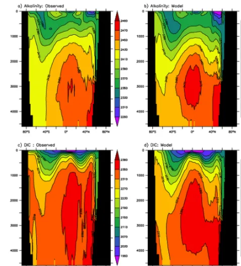
Figure A1. Comparison of the observed alkalinity (a) and

prein-dustrial dissolved inorganic carbon (c) (Key et al., 2004) with the REF simulation in the year 1850 for alkalinity (b) and dissolved inorganic carbon (d) in units of mmol m−3.

In the photic zone, which is set to be the surface layer of the model (upper 50 m), the biological production of par-ticulate organic matter and parpar-ticulate inorganic carbon oc-curs. For particulate organic matter, the production of partic-ulate organic phosphorus (POP) was defined by the following equations:

Vmax=0.6(1.066)T (A3)

F (I )=[1−eG(I )] (A4)

G(I )=I (x, t )αPAR

Vmax

(A5)

QP_O=S_nppo VmaxMin[

P P+Pk

, F (I )] (A6)

EPOP=QPO1z (A7)

up-Figure A2. Comparison of the global averaged profiles of the REF

simulation in the year 1850 with the observations for (a) preindus-trial dissolved inorganic carbon; (b) dissolved oxygen and appar-ent oxygen utilisation; (c) phosphate and (d) alkalinity in units of mmol m−3. The observed fields come from (Key et al., 2004) and (Boyer et al., 2009).

take of phosphate for POP production in mmol P m−3day−1 in the photic zone.QP_O is a function of a growth limitation function, a maximum temperature-dependent phytoplankton growth rate and a constant (S_nppo ). The growth limitation function uses the minimum value of light- and phosphate-limited growth. The phosphate-phosphate-limited growth term is based on the phosphate concentration of the surface layerP and the half saturation uptake (Pk) value for phosphate utilisation, which was set to 0.1 mmol P m−3_{. The constant S}o

npp con-verts the phytoplankton growth rate into organic matter avail-able for export and its value (0.005 mmol P m−3_{) was} manu-ally tuned to satisfactorily reproduce the observed phosphate and oxygen concentrations. Finally,EPOPgives the produc-tion of particulate organic phosphorous in the photic zone (mmol P m−2day−1), where1zis the thickness of the sur-face layer in metres (50 m).

The POP uptake in the photic zone was linked to inorganic carbon, oxygen and alkalinity uptake in the photic zone by the following equations:

QC_O=106QP_O (A8)

QO_O= −136QP_O (A9)

QA_O= −16QP_O (A10)

Particulate inorganic carbon production in the model was linked to particulate organic carbon (POC) production by us-ing a fixed rain ratio (ro) of 9 % (Yamanaka and Tajika, 1996) as follows:

EPOC=106QPO1z =QCO1z (A11)

EPIC=ro×106QPO1z =ro×QCO1z (A12) to give the following uptake of inorganic carbon and alkalin-ity in the photic zone:

QC_I =ro×106QP_O (A13)

QA_I =rv×2×106QP_O, ro=0.09 (A14) The POP, POC and PIC produced in the photic zone were vertically exported from the photic zone and instantaneously remineralised in the ocean interior according to the following equations.

QP_O=EPOC/106

∂

∂z[R(z)] (A15)

QC_O=EPOC

∂

∂z[R(z)] (A16)

QC_I =EPIC

∂

∂z[D(z)], (A17)

where

R(z)= z

100m

REMINPOC

(A18)

D(z)=exp(z/REMINPIC) (A19)

are normalised vertical depth profiles of POC and PIC, re-spectively, z is depth in metres, REMINPOC = −0.9 sets the remineralisation length scale of POC and REMINPIC = 3500 m sets the depth scale for PIC dissolution (Yamanaka and Tajika, 1996).

There is no remineralisation above 100 m and all the POM and PIC reaching the ocean bottom are remineralised in the bottom layer of the model. The relationship between POC remineralisation and phosphate, oxygen and alkalinity is given by Eqs. (A8–A10).

Further, the remineralisation of POC also occurs in anoxic regions through denitrification. This occurs by remineralis-ing the POM back into its inorganic constituents without con-suming any oxygen. The remineralisation of POM in the den-itrification regions increases alkalinity in the same manner as the aerobic respiration (Eq. A10), which is not correct (Paul-mier et al., 2009) but the error is actually small and it was done to ensure alkalinity was conserved in the ocean.

Acknowledgements. Funding for this work was provided by the

Australian Climate Change Science Program, the Pacific-Australia Climate Change Science and Adaptation Planning Program, and the CSIRO Wealth from Oceans Flagship.

Edited by: M. Grégoire

References

Archer, D. E., Eshel, G., Winguth, A., Broecker, W., Pierrehumbert, R., Tobis, M., and Jacob, R.: AtmosphericpCO(2) sensitivity to the biological pump in the ocean, Global Biogeochem. Cy., 14, 1219–1230, 2000.

Armstrong, R. A., Lee, C., Hedges, J. I., Honjo, S., and Wakeham, S. G.: A new, mechanistic model for organic carbon fluxes in the ocean based on the quantitative association of POC with ballast minerals, Deep Sea Res. Pt. II, 49, 219–236, 2002.

Arnold, H. E., Kerrison, P., and Steinke, M.: Interacting effects of ocean acidification and warming on growth and DMS-production in the haptophyte coccolithophore Emiliania huxleyi, Glob. Change Biol., 19, 1007–1016, 2013.

Aumont, O. and Bopp, L.: Globalizing results from ocean in situ iron fertilization studies, Global Biogeochem. Cycles, 20, GB2017, doi:10.1029/2005GB002591, 2006.

Bellerby, R. G. J., Schulz, K. G., Riebesell, U., Neill, C., Nondal, G., Heegaard, E., Johannessen, T., and Brown, K. R.: Marine ecosystem community carbon and nutrient uptake stoichiometry under varying ocean acidification during the PeECE III exper-iment, Biogeosciences, 5, 1517–1527, doi:10.5194/bg-5-1517-2008, 2008.

Bopp, L., Quere, C. L., Heimann, M., Manning, A. C., and Monfray, P.: Climate-induced oceanic oxygen fluxes: Implications for the contemporary carbon budget, Global Biogeochem. Cy., 16, 1022, doi:10.1029/2001GB001445, 2002.

Bopp, L., Resplandy, L., Orr, J. C., Doney, S. C., Dunne, J. P., Gehlen, M., Halloran, P., Heinze, C., Ilyina, T., Séférian, R., Tjiputra, J., and Vichi, M.: Multiple stressors of ocean ecosys-tems in the 21st century: projections with CMIP5 models, Biogeosciences, 10, 6225–6245, doi:10.5194/bg-10-6225-2013, 2013.

Boyer, T. P., Antonov, J. I., Baranova, O. K., Garcia, H. E., Johnson, D. R., Locarnini, R. A., Mishonov, A. V., O’Brien, T., Seidov, D., and Smolyar, I. V.: World Ocean Database 2009, Vol. 66, NOAA Atlas NESDIS, U.S. Gov. Printing Office, Wash., D.C., 2009. Breitbarth, E., Bellerby, R. J., Neill, C. C., Ardelan, M. V.,

Meyerhöfer, M., Zöllner, E., Croot, P. L., and Riebesell, U.: Ocean acidification affects iron speciation during a coastal sea-water mesocosm experiment, Biogeosciences, 7, 1065–1073, doi:10.5194/bg-7-1065-2010, 2010.

Brewer, P. G. and Peltzer, E. T.: Oceans: Limits to marine life, Sci-ence, 324, 347–348, 2009.

Brohan, P., Kennedy, J. J., Harris, I., Tett, S. F. B., and Jones, P. D.: Uncertainty estimates in regional and global observed temper-ature changes: A new data set from 1850, J. Geophys. Res.-Atmos., 111, D12106, doi:10.1029/2005JD006548, 2006. Caldeira, K.: Ocean model predictions of chemistry changes from

carbon dioxide emissions to the atmosphere and ocean, J. Geo-phys. Res., 110, C09S04, 2005.

Cameron-Smith, P., Elliott, S., Maltrud, M., Erickson, D., and Wingenter, O.: Changes in dimethyl sulfide oceanic distribu-tion due to climate change, Geophys. Res. Lett., 38, L07704, doi:10.1029/2011GL047069, 2011.

Canadell, J. G., Le Quere, C., Raupach, M. R., Field, C. B., Buiten-huis, E. T., Ciais, P., Conway, T. J., Gillett, N. P., Houghton, R. A., and Marland, G.: Contributions to accelerating atmo-spheric CO2 growth from economic activity, carbon intensity, and efficiency of natural sinks, P. Natl. Acad. Sci. USA, 104, 18 866–18 870, 2007.

Cocco, V., Joos, F., Steinacher, M., Frölicher, T. L., Bopp, L., Dunne, J., Gehlen, M., Heinze, C., Orr, J., Oschlies, A., Schnei-der, B., SegschneiSchnei-der, J., and Tjiputra, J.: Oxygen and indicators of stress for marine life in multi-model global warming projec-tions, Biogeosciences, 10, 1849–1868, doi:10.5194/bg-10-1849-2013, 2013.

Dentener, F.: Global maps of atmospheric nitrogen deposition, 1860, 1993, and 2050, Data set, available at: http://daac.ornl.gov/ from Oak Ridge National Laboratory Distributed Active Archive Center, Oak Ridge, Tennessee, USA, 2006.

Doney, S. C., Fabry, V. J., Feely, R. A., and Kleypas, J. A.: Ocean Acidification: The Other CO2Problem, Annu. Rev. Mar. Sci., 1, 169–192, 2009.

Duteil, O., Koeve, W., Oschlies, A., Aumont, O., Bianchi, D., Bopp, L., Galbraith, E., Matear, R., Moore, J. K., Sarmiento, J. L., and Segschneider, J.: Preformed and re-generated phosphate in ocean general circulation models: can right total concentrations be wrong?, Biogeosciences, 9, 1797–1807, doi:10.5194/bg-9-1797-2012, 2012.

Duteil, O., Koeve, W., Oschlies, A., Bianchi, D., Galbraith, E., Kri-est, I., and Matear, R.: A novel estimate of ocean oxygen utilisa-tion points to a reduced rate of respirautilisa-tion in the ocean interior, Biogeosciences, 10, 7723–7738, doi:10.5194/bg-10-7723-2013, 2013.

Fabry, V., Seibel, B., Feely, R., and Orr, J.: Impacts of ocean acidi-fication on marine fauna and ecosystem processes, ICES J. Mar. Sci. 65, 414–432, 2008.

Gabric, A., Murray, N., Stone, L., and Kohl, M.: Modelling the proeduction of dimethylsulfide during a phytoplankton bloom, J. Geophys. Res., 98, 22805–22816, 1993.

Gabric, A., Qu, B., Matrai, P., and Hirst, A.: The simulated re-sponse of dimethylsulfide production in the Arctic Ocean to global warming, Tellus B, 57, 391–403, 2011.

Gehlen, M., Gruber, N., Gangstø, R., Bopp, L., and Oschlies, A.: Biogeochemical consequences of ocean acidification and feed-backs to the earth system, in: Ocean Acidification, vol. 1, edited by: Gattuso, J.-P. and Hansson, L., 230–248, Oxford University Press, 2011.

Glessmer, M. S., Eden, C., and Oschlies, A.: Contribution of oxygen minimum zone waters to the coastal upwelling off Mauritania, Prog. Oceanogr., 83, 143–150, 2009.

Gruber, N. and Galloway, J.: An earth-system perspective of the global nitrogen cycle, Nature, 451, 293–296, 2008.

Guinotte, J. M., Buddemeier, R. W., and Kleypas, J. A.: Future coral reef habitat marginality: temporal and spatial effects of climate change in the Pacific basin, Coral Reefs, 22, 551–558, doi:10.1007/s00338-003-0331-4, 2003.

Heinze, C.: Simulating oceanic CaCO₃ export production in the greenhouse, Geophys. Res. Lett., 31, L16308, doi:10.1029/2004GL020613, 2004.

Hoffmann, L. J., Breitbarth, E., Boyd, P. W., and Hunter, K. A.: Influence of ocean warming and acidification on trace metal biogeochemistry, Mar. Ecol.-Prog. Ser., 470, 191–205, doi:10.3354/meps10082, 2012.

Hopkins, F., Nightingale, P., and Liss, P.: Effects of ocean acidifica-tion on the marine source of atmospherically active trace gases, in: Ocean Acidification, edited by: Gattuso, J.-P. and Hansson, L., p. 210, Oxford University Press, 2011.

Hutchins, D. A.: Oceanography: forecasting the rain ratio, Nature, 476, 41–42, 2011.

Hutchins, D. A., Mulholland, M. R., and Fu, F.: Nutrient cycles and marine microbes in a CO2-enriched ocean, Oceanography, 22, 128–145, 2009.

Key, R. M., Kozyr, A., Sabine, C. L., Lee, K., Wanninkhof, R., Bullister, J. L., Feely, R. A., Millero, F. J., Mordy, C., and Peng, T. H.: A global ocean carbon climatology: Results from Global Data Analysis Project (GLODAP), Global Biogeochem. Cy., 18, GB4031, doi:10.1029/2004GB002247, 2004.

Khatiwala, S., Primeau, F., and Hall, T.: Reconstruction of the his-tory of anthropogenic CO2concentrations in the ocean, Nature, 462, 346–349, 2009.

Kloster, S., Six, K. D., Feichter, J., Maier-Reimer, E., Roeckner, E., Wetzel, P., Stier, P., and Esch, M.: Response of dimethylsulfide (DMS) in the ocean and atmosphere to global warming, J. Geo-phys. Res., 112, G03005, doi:10.1029/2006JG000224, 2007. Lawrence, P. J., Feddema, J. J., Bonan, G. B., Meehl, G. A.,

O’Neill, B. C., Oleson, K. W., Levis, S., Lawrence, D. M., Kluzek, E., Lindsay, K., and Thornton, P. E.: Simulating the bio-geochemical and biogeophysical impacts of transient land cover change and wood harvest in the Community Climate System Model (CCSM4) from 1850 to 2100, J. Climate, 25, 3071–3095, 2013.

Mao, J., Phipps, S. J., Pitman, A. J., Wang, Y. P., Abramowitz, G., and Pak, B.: The CSIRO Mk3L climate system model v1.0 coupled to the CABLE land surface scheme v1.4b: evaluation of the control climatology, Geosci. Model Dev., 4, 1115–1131, doi:10.5194/gmd-4-1115-2011, 2011.

Matear, R. J. and Elliott, B.: Enhancement of oceanic uptake of anthropogenic CO₂by macro-nutrient fertilization, J. Geophys. Res., 109, C4001, doi:10.1029/2000JC000321, 2004.

Matear, R. J. and Hirst, A. C.: Climate Change Feedback on the Future Oceanic CO2uptake, Tellus, 51B, 722–733, 1999. Matear, R. J. and Hirst, A. C.: Long term changes in

dis-solved oxygen concentrations in the ocean caused by pro-tracted global warming, Global Biogeochem. Cy., 17, 1125, doi:10.1029/2002GB001997, 2003.

Matear, R. J. and Wong, C. S.: Potential to increase the oceanic CO₂uptake by enhancing marine productivity in high nutrient low chlorophyll regions, 249–253, 1999.

Matear, R. J., Hirst, A. C., and McNeil, B. I.: Changes in dis-solved oxygen in the Southern Ocean with climate change, Geochemistry Geophysics Geosystems (http://gcubed.magnet. fsu.edu/main.html), 1, 2000.

Matear, R. J., Wang, Y.-P., and Lenton, A.: Land and ocean nutri-ent and carbon cycle interactions, Curr. Op. Environ. Sustain., 2, 258–263, 2010.

Matsumoto, K., Sarmiento, J. L., Key, R. M., Aumont, O., Bullis-ter, J. L., Caldeira, K., Campin, J. M., Doney, S. C., Drange, H., Dutay, J. C., Follows, M. J., Gao, Y., Gnanadesikan, A., Gru-ber, N., Ishida, A., Joos, F., Lindsay, K., Maier-Reimer, E., Marshall, J. C., Matear, R. J., Monfray, P., Mouchet, A., Naj-jar, R., Plattner, G. K., Schlitzer, R., Slater, R., Swathi, P. S., Totterdell, I. J., Weirig, M. F., Yamanaka, Y., Yool, A., and Orr, J. C.: Evaluation of ocean carbon cycle models with data-based metrics, Geophys. Res. Lett., 31, L07303, doi:10.1029/2003GL018970, 2004.

Najjar, R. G., Jin, X., Louanchi, F., Aumont, O., Caldeira, K., Doney, S. C., Dutay, J. C., Follows, M. J., Gruber, N., Joos, F., Lindsay, K., Maier-Reimer, E., Matear, R. J., Matsumoto, K., Monfray, P., Mouchet, A., Orr, J. C., Plattner, G. K., Sarmiento, J. L., Schlitzer, R., Slater, R. D., Weirig, M. F., Yamanaka, Y., and Yool, A.: Impact of circulation on export production, dis-solved organic matter, and disdis-solved oxygen in the ocean: Results from Phase II of the Ocean Carbon-cycle Model Intercompari-son Project (OCMIP-2), Global Biogeochem. Cy., 21, GB3007, doi:10.1029/2006GB002857, 2007.

Orr, J. C., Fabry, V. J., Aumont, O., Bopp, L., Doney, S. C., Feely, R. A., Gnanadesikan, A., Gruber, N., Ishida, A., Joos, F., Key, R. M., Lindsay, K., Maier-Reimer, E., Matear, R. J., Monfray, P., Mouchet, A., Najjar, R. G., Plattner, G. K., Rodgers, K. B., Sabine, C. L., Sarmiento, J. L., Schlitzer, R., Slater, R. D., Totterdell, I. J., Weirig, M. F., Yamanaka, Y., and Yool, A.: Anthropogenic ocean acidification over the twenty-first century and its impact on calcifying organisms, Nature, 437, 681–686, 2005.

Oschlies, A., Schulz, K. G., Riebesell, U., and Schmittner, A.: Simulated 21st century’s increase in oceanic suboxia by CO2 -enhanced biotic carbon export, Global Biogeochem. Cy., 22, GB4008, doi:10.1029/2007GB003147, 2008.

Paulmier, A., Kriest, I., and Oschlies, A.: Stoichiometries of remineralisation and denitrification in global biogeochemical ocean models, Biogeosciences, 6, 923–935, doi:10.5194/bg-6-923-2009, 2009.

Phipps, S. J., Rotstayn, L. D., Gordon, H. B., Roberts, J. L., Hirst, A. C., and Budd, W. F.: The CSIRO Mk3L climate system model version 1.0 – Part 1: Description and evaluation, Geosci. Model Dev., 4, 483–509, doi:10.5194/gmd-4-483-2011, 2011. Pinsonneault, A. J., Matthews, H. D., Galbraith, E. D., and

Schmittner, A.: Calcium carbonate production response to future ocean warming and acidification, Biogeosciences, 9, 2351–2364, doi:10.5194/bg-9-2351-2012, 2012.

Pitman, A. J., Avila, F. B., Abramowitz, G., Wang, Y. P., Phipps, S. J., and de Noblet-Ducoudré, N.: Importance of back-ground climate in determining impact of land-cover change on regional climate, Nat. Clim. Change, 1, 472–475, 2011. Portner, H. O. and Farrell, A. P.: ECOLOGY:

physi-ology and climate change, Science, 322, 690–692, doi:10.1126/science.1163156, 2008.

Raven, J. A.: Ocean Acidification Due to Increasing Atmospheric Carbon Dioxide, R Society (Great Britain), 60 pp., 2005. Redfield, A. C.: On the proportions of organic derivatives in sea

water and their relation to the composition of plankton, in James Johnstone Memorial Volume, ed. R. J. Daniel, 172–192, 1934. Ridgwell, A., Schmidt, D. N., Turley, C., Brownlee, C.,

ma-nipulations to Earth system models: scaling calcification im-pacts of ocean acidification, Biogeosciences, 6, 2611–2623, doi:10.5194/bg-6-2611-2009, 2009.

Riebesell, U., Schulz, K. G., Bellerby, R. G. J., Botros, M., Fritsche, P., Meyerhofer, M., Neill, C., Nondal, G., Oschlies, A., Wohlers, J., and Zollner, E.: Enhanced biological carbon con-sumption in a high CO2ocean, Nature, 450, 545–549, 2007. Rivkin, R. B.: Biogenic Carbon Cycling in the Upper Ocean: Effects

of Microbial Respiration, Science, 291, 2398–2400, 2001. Rost, B., Zondervan, I., and Wolf-Gladrow, D.: Sensitivity of

phyto-plankton to future changes in ocean carbonate chemistry: current knowledge, contradictions and research directions, Mar. Ecol.-Prog. Ser., 373237., 227, 227–237, 2008.

Schmittner, A., Oschlies, A., Matthews, H. D., and Galbraith, E. D.: Future changes in climate, ocean circulation, ecosystems, and biogeochemical cycling simulated for a business-as-usual CO2 emission scenario until year 4000 AD, Global Biogeochem. Cy., 22, GB1013, doi:10.1029/2007GB002953, 2008.

Shi, D., Xu, Y., Hopkinson, B., and Morel, F.: Effect of ocean acid-ification on iron availability to marine phytoplankton, Science, 327, 676, doi:10.1126/science.1183517,, 2010.

Six, K. D., Kloster, S., Ilyina, T., Archer, S. D., Zhang, K., and Maier-Reimer, E.: Global warming amplified by reduced sulphur fluxes as a result of ocean acidification, Nat. Clim. Change, 3, 1–4, 2013.

Tagliabue, A., Bopp, L., and Gehlen, M.: The response of marine carbon and nutrient cycles to ocean acidification: large uncertain-ties related to phytoplankton physiological assumptions, Global Biogeochem. Cy., 25, GB3017, doi:10.1029/2010GB003929, 2011.

Taylor, K. E.: Summarizing multiple aspects of model performance in a single diagram, J. Geophys. Res.-Atmos., 106, 7183–7192, 2001.

Trenberth, K. E., Jones, P. D., Ambenje, P., Bojariu, R., Easter-ling, D., Tank, A. K., Parker, D., Rahimzadeh, F., Renwick, J. A., Rusticucci, M., Soden, B., and Zhai, P.: Observations: Surface and Atmospheric Climate Change, 2007.

Trull, T. W., Bray, S. G., Manganini, S. J., Honjo, S., and Fran-cois, R.: Moored sediment trap measurements of carbon export in the Subantarctic and Polar Frontal Zones of the Southern Ocean, south of Australia, J. Geophys. Res.-Atmos., 106, 31489–31509, 2001.

Wang, Y. P., Law, R. M., and Pak, B.: A global model of carbon, nitrogen and phosphorus cycles for the terrestrial biosphere, Bio-geosciences, 7, 2261–2282, doi:10.5194/bg-7-2261-2010, 2010. Wanninkhof, R.: Relationship between wind speed and gas ex-change over the ocean, J. Geophys. Res., 97, 7373–7382, 1992. Weinbauer, M. G., Mari, X., and Gattuso, J.-P.: Effects of ocean

acidification on the diversity and activity of heterotrophic marine microorganisms, in: Ocean Acidification, edited by: Gattuso, J.-P. and Hansson, L., Oxford University Press, 2011.

Weiss, R. F.: The solubility of nitrogen, oxygen and argon in water and seawater, Deep Sea Res., 17, 721–735, 1970.

Yamanaka, Y. and Tajika, E.: The role of the vertical fluxes of par-ticulate organic matter and calcite in the oceanic carbon cycle: studies using a ocean biogeochemical general circulation model, Global Biogeochem. Cy., 10, 361–382, 1996.

Zaehle, S., Friedlingstein, P., and Friend, A. D.: Terrestrial nitrogen feedbacks may accelerate future climate change, Geophys. Res. Lett., 37, L01401, doi:10.1029/2009GL041345, 2010.

Zhang, Q., Wang, Y. P., Matear, R. J., Pitman, A. J., and Dai, Y. J.: Nitrogen and phosphorous limitations significantly re-duce future allowable CO₂ emissions, Geophys. Res. Lett., doi:10.1002/2013GL058352, 2014.