Rui Wu1, Lei Yang2, Chao Chen3, Sajjad Ahmad4, Sergiu M. Dascalu2, and Frederick C. Harris Jr.2 1Department of Computer Science, East Carolina University, Greenville, NC, USA
2Department of Computer Science & Engineering, University of Nevada – Reno, Reno, NV, USA 3Department of Geosciences, Boise State University, Boise, ID, USA
4Department of Civil and Environmental Engineering and Construction, University of Nevada – Las Vegas, Las Vegas, NV, USA
Correspondence:Rui Wu ([email protected]) Received: 5 June 2018 – Discussion started: 10 August 2018
Revised: 18 June 2019 – Accepted: 29 July 2019 – Published: 23 September 2019
Abstract.This paper studies how to improve the accuracy of hydrologic models using machine-learning models as post-processors and presents possibilities to reduce the workload to create an accurate hydrologic model by removing the cal-ibration step. It is often challenging to develop an accurate hydrologic model due to the time-consuming model calibra-tion procedure and the nonstacalibra-tionarity of hydrologic data. Our findings show that the errors of hydrologic models are correlated with model inputs. Thus motivated, we propose a modeling-error-learning-based post-processor framework by leveraging this correlation to improve the accuracy of a hy-drologic model. The key idea is to predict the differences (errors) between the observed values and the hydrologic model predictions by using machine-learning techniques. To tackle the nonstationarity issue of hydrologic data, a moving-window-based machine-learning approach is proposed to en-hance the machine-learning error predictions by identifying the local stationarity of the data using a stationarity measure developed based on the Hilbert–Huang transform. Two hy-drologic models, the Precipitation–Runoff Modeling System (PRMS) and the Hydrologic Modeling System (HEC-HMS), are used to evaluate the proposed framework. Two case stud-ies are provided to exhibit the improved performance over the original model using multiple statistical metrics.
1 Introduction 1.1 Motivation
Hydrologic models are commonly used to simulate environ-mental systems, which help us to understand water systems and their responses to external stresses. They are also widely used in scientific research for physical process studies and environmental management for decision support and policy-making (Environmental Protection Agency, 2017). One of the most important criteria for model performance evalua-tions is prediction accuracy. A reliable model is able to cap-ture the hydrologic feacap-tures with robust and stable predic-tions. However, it is challenging to develop a reliable hy-drologic model with low biases and variances. In this pa-per, we aim to develop a post-processor framework, named MELPF, which is short for Modeling Error Learning based Post-Processor Framework, to improve the reliability of hy-drologic models.
calibra-patterns that are highly correlated with model inputs (see Fig. 3). Such patterns can be learned via machine learning (see Sect. 2) and applied in predictions. Thus motivated, we propose that MELPF can learn the modeling error to enhance the prediction accuracy.
Despite the potential improvement brought by learning techniques, it is worth noting that pure machine-learning techniques cannot completely replace hydrologic models. When we compare the performance of the environ-mental model and machine-learning methods, it turns out that the accuracy of the Precipitation–Runoff Modeling Sys-tem (PRMS) (Leavesley et al., 1983; Markstrom et al., 2005, 2015) is much higher than that of commonly used machine-learning techniques (e.g., random forest tree, Breiman, 2001; gradient-boosted tree, Hastie et al., 2009). Compared to hy-drologic models developed using domain knowledge, pure machine-learning models with limited training data cannot accurately characterize all the features of the underlying physical process. Nevertheless, based on hydrologic simu-lation, machine-learning approaches are able to further en-hance hydrologic model results by predicting the original modeling errors via learning the relationships between model inputs and output simulation results. In the hydrologic mod-eling results, the term “simulations” is widely used for both concepts of historical record replication and future predic-tion.
1.2 Major contributions
In this paper, we develop a modeling-error-learning-based post-processor framework to enhance the prediction accu-racy of hydrologic models. Based on the results in Sect. 3, the proposed MELPF can ease the parameter tuning pro-cesses and achieve accurate predictions. The key idea is to leverage the correlation between the hydrologic model in-puts and model output errors. There are two main challenges of building the proposed framework: (1) how to improve the efficiency and accuracy in a hydrologic model in terms of model simulation and development and (2) how to deal with the nonstationary hydrologic data. To solve the first chal-lenge, we propose a machine-learning-based post-processor, which can capture and characterize model errors to improve hydrologic model predictions. This can help to avoid the misleading effects of irrelevant model inputs. Also, we
pro-– MELPF is developed to improve the prediction accu-racy and flexibility of hydrologic models. One common issue of existing hydrologic simulation studies is that the development of hydrologic models, in terms of cali-bration processes, often requires long research time cy-cles but ends up with barely satisfied model accuracy. To tackle these challenges, the proposed MELPF can significantly simplify the parameter tuning processes by learning and calibrating the modeling error using machine-learning techniques. Moreover, the proposed MELPF can use different machine-learning methods for different scenarios to obtain the best results, and the model parameters can be dynamically updated using the latest data. Our experiment results in Sect. 3 show that our method can significantly improve prediction accu-racy compared with the simulation results of existing hydrologic models.
– A moving-window-based machine-learning approach is proposed, which can enhance the performance of the machine-learning technique when dealing with nonsta-tionary hydrologic data. We observe that the distribu-tion of hydrologic data changes over time and the data exhibit seasonality (see Fig. 2). The proposed moving-window-based machine-learning approach can charac-terize the time-varying relationship between the model inputs and model output errors. The key step is to choose a suitable window size within which the data are stationary, as most machine-learning techniques are designed for stationary data. By leveraging recent ad-vances in the field of nonlinear and nonstationary time series analysis, particularly HHT, we propose the degree of stationarity to measure the local stationarity of the data. Based on the degree of stationarity and the auto-correlation, we propose a window size selection method to optimize the performance of the machine-learning techniques.
are some methods that perform well but can only be applied to a certain machine-learning method, such as Klinkenberg and Joachims (2000) and Bifet Figuerol and Gavaldà Mestre (2009). Bifet Figuerol and Gavaldà Mestre (2009) proposed a concept-drift-based method to dynamically adapt the win-dow size for a Hoeffding tree (Domingos and Hulten, 2000). To solve the limitation, some methods are proposed that can be applied to different machine-learning techniques by using statistical techniques to monitor the concept drifts. In Klinkenberg and Renz (1998), Lanquillon (2001), and Bouchachia (2011), statistical process control (SPC; Oak-land, 2007) is leveraged to monitor the data change rate by using the error rate. If the error rate change is larger than a threshold, it means the data are not stable, and then the window size should be changed. These methods need to as-sume that the error rate follows a certain distribution, and then calculate the threshold by using the error confidence in-terval. Similarly, in Gama et al. (2004) and Bifet and Gavalda (2007), window selection methods are proposed based on the concept of context with the stationary distribution. The pro-posed methods require the dataset inside a window to follow a certain distribution, and then calculate the confidence in-terval by using an approximate measurement (Gama et al., 2004; Bifet and Gavalda, 2007). However, this requirement may not be satisfied for some hydrologic data because the data distributions may be not known or follow a certain dis-tribution. Different from these works, we choose the window size based on the degree of stationarity of the data according to the proposed stationarity measure (see Sect. 2.2.2), which does not that assume the data follow any predetermined dis-tribution and is applicable to different machine-learning tech-niques.
There are many methods to improve the performance of hydrologic model simulations by reducing uncertainties from various sources: model input preprocessing, data assimila-tion, model calibraassimila-tion, and model result post-processing (Ye et al., 2014). Model input preprocessing deals with uncer-tainties from model input variables such as establishing pre-cipitation measurement networks or post-processing meteo-rological predictions (Glahn et al., 2009). Data assimilation treats the uncertainties from model initial and boundary con-ditions. For instance, the assimilation of snow water equiva-lence data can improve initial conditions in a snow or
hydro-ples include variants of Bayesian frameworks built on model output (Krzysztofowicz and Maranzano, 2004), the meta-Gaussian approach (Montanari and Brath, 2004), the quan-tile regression approach (Seo et al., 2006), and the wavelet transformation approach (Srivastava et al., 2009). Because the post-processing methodology only deals with model re-sults it requires fewer computations for most cases. There-fore, we propose using the post-processing method in this framework.
sub-Figure 1.A traditional calibrated PRMS model streamflow predic-tion error histogram (example of Lehman Creek).
stantially reduce the performance and reliability of the post-processing algorithms.
The rest of this paper is organized as follows. In Sect. 2, the modeling-error-learning-based post-processor is pro-posed. In Sect. 3, two case studies are presented and the re-sults are analyzed. In Sect. 4, the discussion of our study is provided. The paper is concluded in Sect. 5.
2 Modeling-error-learning-based post-processor framework
Hydrologic models are based on the simulation of water bal-ance among the principal hydrologic components. With dif-ferent study purposes, the selected hydrologic model varies and so do the parameters used in the simulation algorithm. It is challenging to develop an accurate hydrologic model, and traditional hydrologic models can often have high biases and variances in the outputs. By studying many hydrologic scenarios, we observed that hydrologic model errors often follow some patterns that highly correlate with the model in-puts, and such patterns can be learned via machine learning. Thus motivated, we propose that MELPF can learn the mod-eling error to enhance the prediction accuracy. The details of the proposed MELPF are provided in the following section. 2.1 Observations and motivations
We study the prediction errors of a PRMS model (Leavesley et al., 1983; Markstrom et al., 2005, 2015) using 10-year his-torical watershed data collected from USGS (USGS, 2017). The study area is the Lehman Creek watershed in eastern Nevada, and the data are collected every 24 h. Figure 1 illus-trates the error distribution of streamflow prediction from the PRMS model. The distribution is very close to a normal dis-tribution with a close-to-zero mean value and a low variance. However, when taking a closer look at the prediction errors across time (see Fig. 2), we observe a large discrepancy be-tween the model outputs and the ground truths in the middle
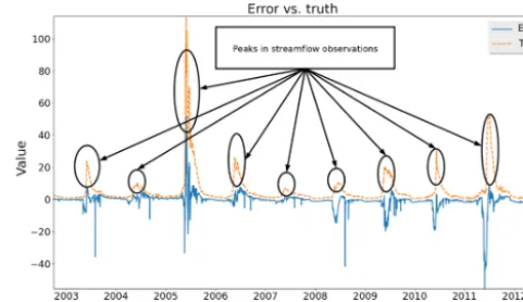
Figure 2.Comparisons between streamflow observations and pre-diction errors from a traditional calibrated PRMS model (example of Lehman Creek). Theyaxis value unit is cubic feet per second.
of each year. It implies that the current PRMS model can-not accurately characterize the streamflow in the middle of a year. Therefore, there is a need to better capture the dynamics of the streamflow in this time period.
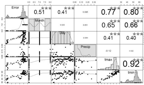
Intuitively, prediction errors contain important informa-tion, which can be leveraged to reduce the hydrologic model errors so as to improve the prediction accuracy. Therefore, we explore the information contained in the prediction errors and find that the prediction errors are actually highly cor-related with the model inputs. As shown in Fig. 3, during May, June, July, and August of the year 2011, the streamflow prediction errors are highly correlated with the temperatures and time (month and day). The larger correlation values and stars in Fig. 3 indicate closer relations between two variables. By leveraging the correlations, we aim to predict the original model errors and thereby improve the prediction accuracy.
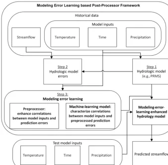
Along this line, we propose using machine-learning tech-niques to learn the modeling errors by leveraging the strong correlations between the prediction errors and the model in-puts in order to improve the accuracy of streamflow predic-tions. The proposed MELPF is illustrated in Fig. 4. It mainly consists of three steps.
– Step 1: develop a hydrologic model, such as PRMS. The model can generate predictions (e.g., streamflow predic-tion) based on the inputs (e.g., temperature, time, and precipitation).
– Step 2: obtain the hydrologic model errors. By compar-ing the ground truths with the hydrologic model predic-tions, MELPF can collect historical hydrologic model errors.
Figure 3.Correlations between PRMS inputs (i.e.,precip,tmax(maximum temperature), andtmin(minimum temperature)) and streamflow prediction errors during May, June, July, and August (2011): the diagonal graphs show the variable distributions, the lower graphs show the scatter plots between the corresponding row and column variables, and the upper values are the correlation values between the corresponding row and column variables (precip: precipitation;tmax: maximum temperature;tmin: minimum temperature); errors: streamflow prediction errors.
After these three steps, the trained machine-learning model is integrated with the original hydrologic model to en-hance the prediction accuracy. It produces improved results by adding the predicted errors with hydrologic model pre-dictions. Different methods in each preprocessor, machine-learning model, and hydrologic model error component can be selected based on the application needs. The details of each component as shown in Fig. 4 are described in the fol-lowing sections.
Remarks. In practice, the development of a hydrologic model needs to be calibrated based on hydrogeologic con-ditions and meteo-hydrologic characteristics. The calibration procedure is a process that finalizes parameters used in the model numerical equations that determine the hydrologic process simulation. With temporal and spatial heterogene-ity, these parameters could either be characterized by both these features, such as in the physically based parameter-distributed hydrologic model PRMS, or be averaged to rep-resent a mean level while still maintaining the capability of capturing the streamflow variation, such as in the Hydrologic Modeling System (HEC-HMS). In this study, the default val-ues of each parameter are used in the uncalibrated cases to compare with the calibrated cases from traditional hy-drologic calibration and post-processor methods. As demon-strated in Sect. 3, the proposed MELPF provides a better
pre-diction accuracy when compared with the traditional hydro-logic calibration method.
2.2 Modeling-error-learning-enhanced hydrologic model
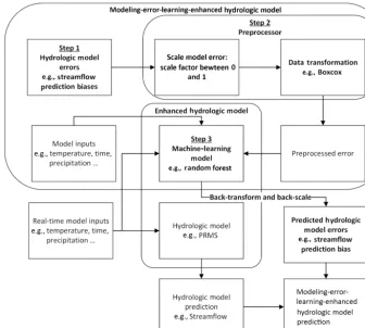
The detailed workflow of the designed modeling-error-learning-enhanced hydrologic model is illustrated in Fig. 5. The basic idea is to use predicted error to calibrate the origi-nal hydrologic model’s predictions, as shown in Eq. (1):
ˆ
pt=f (xt)+g(xt), (1)
wherepˆt denotes the improved prediction at time t; xt
de-notes the model inputs (i.e., temperature, time, and precipi-tation) at timet;f (·)denotes the hydrologic model, which generates predictions based onxt; andg(·)denotes the
er-ror prediction model learned in the machine-learning model component, which generates hydrologic model prediction er-ror based onxt.
As illustrated in Fig. 5, there are basically three steps to building an enhanced hydrologic model.
Figure 4.The diagram of the Modeling Error Learning based Post-Processor Framework.
– Step 2: enhance the correlation between hydrologic model errors and inputs. This step contains two sub-steps: scale model error and data transformation. Scale model error is used to scale error into a certain scope (e.g., between 0 and 1), and data transformation is used to normalize hydrologic model errors and stabilize the variances of hydrologic model errors.
– Step 3: build a machine-learning model. The scaled and transformed original hydrologic model errors and model inputs are used to train a machine-learning model to predict the hydrologic model errors. The predicted errors need to be back-transformed and back-scaled be-fore being used to compensate for the hydrologic model results.
More details of the framework components (rectangles in Fig. 5) and steps (arrows in Fig. 5) are introduced in the fol-low sections.
2.2.1 Preprocessor component
The preprocessor component preprocesses the hydrologic model errors, and the outputs of this component are used to train a machine-learning model in the machine-learning
model component. The objective of the preprocessor com-ponent is to normalize errors and reduce error variances. In other words, this component is used to make it easier for the machine-learning model component to characterize cor-relations between the hydrologic model inputs and errors. Specifically, this component scales and transforms the hy-drologic model prediction errors using Eq. (2):
et =tr(αe), (2)
whereet denotes preprocessed error; tr(·)denotes
transfor-mation function;αdenotes the scaling factor; andedenotes the original hydrologic error. Based on the case studies in Sect. 3, a good scaling factor is often between zero and one.
Figure 5.Modeling-error-learning-enhanced hydrologic model.
Remarks. The preprocessor component should be repeated multiple times to find the best-performing scaling factor and data transformation parameters. For example, percent–time cross-validation can be used to test all possible parameter combination performances (Kohavi, 1995). The performance can be measured by using the root mean square error (RMSE) (Eq. 8), percent bias (PBIAS) (Eq. 9), Nash–Sutcliffe effi-ciency (NSE) (Eq. 10), or coefficient of determination (CD) (Eq. 11). After a good parameter combination is chosen, it will be used in both the preprocessor component and the back-transform and back-scale step.
2.2.2 Machine-learning model component
The machine-learning model component aims to predict the transformed hydrologic model errorg(xˆ t)using the
hydro-logic model inputxt. To obtain the original model prediction
errorg(xt),g(xˆ t)needs to be transformed back using the
in-verse of the transformation function, which is discussed in Sect. 2.2.4. In what follows, we discuss how to findg(ˆ ·) us-ing machine-learnus-ing techniques.
There are many machine-learning techniques that can be applied in this component, such as support vector regression (SVR) (Basak et al., 2007) and gradient-boosted tree (Hastie et al., 2009). Most of them are designed for stationary en-vironments in the sense that the underlying process
fol-lows some stationary probability distribution. However, hy-drologic processes are often nonstationary. As illustrated in Fig. 2, the streamflow shows seasonality in the sense that the patterns of streamflow in each year are similar but change over time. To address this challenge, we propose using a moving time window to adapt to the changes due to hydro-logic data variations.
The basic idea is to set up a time window and train the machine-learning model using the data within the window, which moves over time. By using the time window, we are able to track the changing dynamics of hydrologic data. However, it is challenging to find an appropriate window size. If the window size is too large, it increases model train-ing complexity and the model is not able to quickly adapt to the changes in the hydrologic data. Even though a model with a large window size may generate accurate results dur-ing the traindur-ing phase, it is possible that the accuracy of the model using the test dataset could be very poor, which is due to overfitting issues (Domingos, 2012). If the window size is too small, the model may not be able to capture the pattern of the hydrologic model errors.
Figure 6.Case Study 1, training data autocorrelation values vs. lag days: the data pattern lengths can be 1 year or 2 years because these are the distances between the start point and peaks in the training data.
To find the data pattern, we leverage the autocorrelation of the data. Due to the seasonality, the autocorrelation shows a peak every year (see Fig. 6) and the distance between two peaks indicates that the pattern repeats during this period. However, as illustrated in Fig. 6, there are several peaks, and it remains challenging to determine the window size, i.e., how many peaks should be chosen?
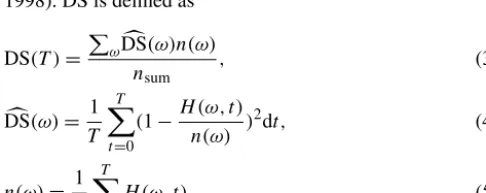
To address this challenge, we further calculate the degree of stationarity of the data in a given window size and use this to determine the window size. Specifically, the degree of sta-tionarity (DS) is defined by leveraging recent advances in the field of nonlinear and nonstationary time series analysis, par-ticularly the Hilbert–Huang transform (HHT) (Huang et al., 1998). DS is defined as
DS(T )= P
ωDS(ω)n(ω)c
nsum , (3)
c
DS(ω)= 1 T
T X
t=0
(1−H (ω, t ) n(ω) )
2dt, (4)
n(ω)= 1 T
T X
t=0
H (ω, t ), (5)
where DS(T )denotes the data stationarity value of window sizeT (Eq. 3),DS can characterize the variation of the datac in a certain frequency (ω) bin over time (Eq. 4), andn(ω)is the average amplitude of the frequency (Eq. 5).
In Eq. (3),nsum=P
ωn(ω). DS(T )sums theDS value ofc each frequency and weights each of them by using n(ω). This ensures that small, relatively insignificant oscillations do not dominate the metric.nsumin the denominator normal-izes DS(T )and allows different DSs to be comparable. Note that the larger DS, the more nonstationary the data, and we prefer a small DS in a given time window.
In Eq. (4),H (ω, t )denotes the Hilbert spectrum, which is a frequency–time distribution of the amplitude of the data. A largeDS indicates large variations in the bin, which meansc
Figure 7.Case Study 1, training data DS vs. window size: 1-year DS is less than 2-year DS. This means the 1-year window contains more stable data and should be chosen.
nonstationary behavior. A close-to-zeroDS indicates smallc variations in the bin, which means stationary behavior.
TheDS concept is first introduced in Huang et al. (1998),c but it only considers the data stationarity of a certain fre-quency bin and does not characterize the entire time series data stationarity. To improve theDS concept, we propose ac DS that calculates the whole dataset stationarity.
After the possible data patterns are chosen based on auto-correlation, the data pattern that has the minimum DS (the most stable) is chosen to be the final window size.
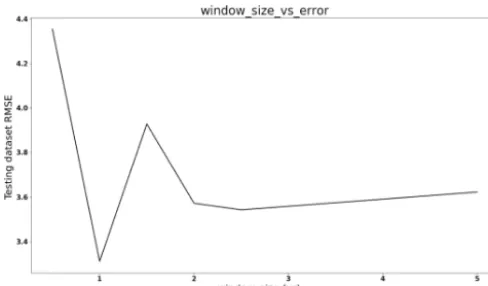
Figure 7 illustrates the values of DS under different wdow sizes for Case Study 1 in Sect. 3.2. The DS value in-creases as the window size grows, which means the data be-come more nonstationary when the window size grows. As the 1-year DS is smaller than 2-year DS, the 1-year window size is chosen for Case Study 1 because it is one of the data patterns and this window size has the minimum DS value. Figure 8 compares the prediction performance using differ-ent window sizes for Case Study 1. It shows the 1-year win-dow size has the best performance. In contrast, the 4.5-year window size is more accurate than the 1-year window size with the training dataset, but the performance is worse with the testing dataset, which means a larger window size can cause overfitting issues.
2.2.3 Back-transform and back-scale
The predicted errors generated from the machine-learning model cannot be used directly because the machine-learning model is trained with the preprocessed errors. The predicted errors need to be back-preprocessed using the corresponding preprocessor methods to obtain the real predicted hydrologic model errors.
Let tr−1denote the inverse of the transformation function; g(xt)can be computed as
g(xt)=tr−1(g(xˆ t))/α, (6)
and the predictionpˆtcan be given as
ˆ
Figure 8.Case Study 1, testing data RMSE vs. window size: the 1-year window size is better than the other window size based on the RMSE value.
2.3 Discussion of proposed methods
Modeling error learning is the key component of MELPF. If it is able to predict the hydrologic model errors, MELPF can improve model results. If not, then MELPF cannot improve a hydrologic model performance. Therefore, if MELPF does not work it is because the modeling error learning nent cannot predict errors accurately. Because this compo-nent leverages the relations between the model inputs and model errors, the component can work when the model in-puts are correlated with the model errors. Therefore, a mod-eler can calculate the correlation values between each model input and the preprocessed model errors of the historical data to test if the proposed MELPF can work. If some model inputs are correlated with the preprocessed model errors, then the proposed MELPF is able to improve the hydrologic model accuracy and vice versa.
How MELPF can perform better is another important question. It depends on the chosen machine-learning tech-niques used in the modeling error learning component. The errors contain biases and variances. Based on bias–variance trade-off theory (Friedman, 1997), when bias decreases, variances will increase and vice versa. Different machine-learning techniques have different characteristics. For exam-ple, a boosted tree has a high bias, low variance, and per-forms well when dimensionality is low; a random forest has a low bias, high variance, and performs well when dimen-sionality is high (Caruana and Niculescu-Mizil, 2005). Thus, the selection of the machine-learning method should be de-termined by the study needs and data characteristics.
However, it is hard to determine which machine-learning technique works better for a certain problem before perform-ing tests. We suggest a pretest to examine which machine-learning technique could work and perform better. The pretest data should be historical data and the size is decided by the data cycle, such as a week, month, and year. For ex-ample, the temperature is high in summer and low in
win-learning model component. Figure 2 is an example of dra-matically changed streamflow. The streamflow observations grow rapidly in the middle of each year and the vibra-tions generate small spikes along the uphills and downhills. The original PRMS model cannot characterize the spikes and generates irregular errors. Because the machine-learning model component is built based on these errors, MELPF can-not perform very well in the middle of every year and gen-erates unnecessary peaks. We propose a method to smooth the hydrologic model predictions to avoid the spikes, which contains three steps.
1. Choose a threshold T, which should be between the maximum and minimum value.
2. Smooth the hydrologic model predictions by usingT. If the difference between the previous prediction and cur-rent prediction is higher thanT, then we use the previ-ous prediction to replace the current prediction.
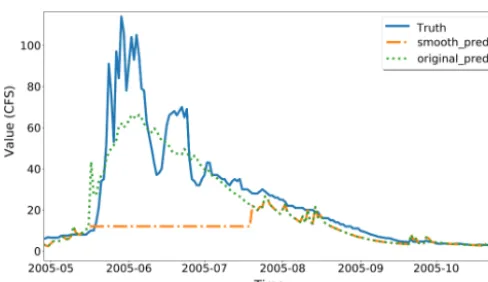
3. Check if the currentT avoids peaks. If the currentT cannot avoid any peaks, then choose a smallerT and go to Step 1. If there is a “plateau” (flat peak) as Fig. 9 displays, then choose a largerT.
When a fittingT is finalized, it is used in both the training phase and in the test phase for the hydrologic model predic-tions. In the training phase, it can help to identify more ap-propriate scale factors, transformation parameters, and win-dow sizes. In the test phase, it can avoid the severe vibration predictions in the original hydrologic model.
3 Results and analysis 3.1 Experiment design
Figure 9.Use 10 as a threshold: there is a plateau around 2005 June generated. CFS is short for cubic feet per second.
parameters are defined by the following equations.
RMSE= v u u t 1 N N X
i=1
(Pi−Ai)2 (8)
PBIAS=
N P
i=1
(Ai−Pi)100
N P
i=1 Ai
(9)
NSE=1−
N P
i=1
(Ai−Pi)2
N P
i=1
(Ai−A)2
(10)
CD=
N P
i=1
(Ai−Pi)(Pi−P )
N
P
i=1
(Ai−A)2 12 N
P
i=1
(Pi−P )2 12
2
(11)
Pi andAi represent the simulated and observed values,
re-spectively;Ais the mean of the observed values andP is the mean of simulated values for the entire evaluation period.
RMSE measures how close the observed data are to the predicted values while retaining the original units of the model’s output and observed data. Lower values of RMSE indicate a better fit of the model. RMSE is one of the impor-tant standards that defines how accurately the model predicts the response, and it is commonly used in many fields.
PBIAS is a measure to evaluate the model simulations. It determines whether the predictions are underestimated or overestimated compared to the actual observations. If the PBIAS values are positive, the model overestimates the re-sults; otherwise, the model underestimates the results by the given percentage. Therefore, values closer to zero are pre-ferred for PBIAS.
The Nash–Sutcliffe efficiency (NSE) is a normalized statistic assessing the model’s ability to make predictions that
higher CD values indicate better results.
In the following case studies, we also provide the predic-tion interval (PI), which offers the possible predicpredic-tion range. The PI is calculated using Eq. (12), whereX is the sample mean,nis the number of samples, andTais a Student’s
t-distribution percentile withn−1 degrees of freedom. PI is described with an upper bound and lower bound.
PI=Xn±Tasn p
1+(1/n) (12)
3.2 Case Study 1
3.2.1 The PRMS hydrologic model
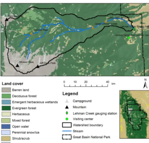
The Precipitation–Runoff Modeling System (PRMS) was de-veloped by the US Geological Survey in the 1980s, which is a physically based parameter-distributed hydrologic model-ing system (Leavesley et al., 1983; Markstrom et al., 2005, 2015). The PRMS model used in this study was developed by Chen et al. (2015a) in the study area of Lehman Creek watershed, eastern Nevada. The watershed is located in the Great Basin National Park, occupying an area of 5839 ac of the southern Snake Valley (Prudic et al., 2015; Volk, 2014). More than 78 % of the land cover was evergreen forest, de-ciduous forest, and mixed forest; 2 % was shrubs, 2 % was perennial snow and ice, and 17 % was barren land (Chen et al., 2016; Chen et al., 2015a). The streamflow is mainly composed of snowmelt, which is sourced from the high el-evated area in the west, flowing over the large mountain quartzite and recharging the groundwater system through al-luvial deposits and karst–limestone in the east (Chen et al., 2017). These high hydro-geography variations made it ap-propriate to use the PRMS model to describe the spatial het-erogeneity of hydrologic processes. Figure 10 displays the study area.
hydro-Figure 10.PRMS hydrologic model study area, which was derived from the vegetation map obtained from the National Land Cover Database (NLCD, 2011) with 30 m resolution. The map is drawn based on data from Yang et al. (2018).
logic component on each of 4704 units (Chen et al., 2015a). Among all the parameters required for model runs, some pa-rameters are specifically sensitive and have a great influence on the model simulation results. Such parameters determine the temporal and/or spatial distribution of precipitation and require specification on every one of 12 months and/or ev-ery one of 4704 cells (e.g., tmax_allsnow, monthly maxi-mum air temperature when precipitation is assumed to be snow;snow_adj/rain_adj, monthly factor to adjust measured precipitation on each hydrologic response unit (HRU) to ac-count for differences in elevation, and so forth; tmin_lapse, monthly values representing the change in minimum air tem-perature per 1000elev_unitsof elevation change).
One station’s meteorologic data were used as the driving forces to the developed model in the study area of Lehman Creek watershed. Daily precipitation, maximum tempera-ture, and minimum temperature from 1 October 2003 to 30 September 2012 were collected from the meteorologic station (no. 263340, Great Basin NP). Daily streamflows at the Lehman Creek Baker gauging station (no. 10243260) were collected for model calibration and validation (Chen et al., 2015a).
3.2.2 Results
The goal is to improve the PRMS model streamflow pre-dictions. First, the training dataset is transformed by using log-sinh transformation, which is introduced in Wang et al. (2012). Equation (13) is the transformation equation and
Figure 11.Case Study 1, final PRMS model streamflow prediction improvements. The improved predictions are closer to the ground truth than the original predictions.
Eq. (14) is the back-transformation equation.
ˆ
y=log(sinh[a+by])
b (13)
y=sinh
−1(10ybˆ )−a
b (14)
Here,a andbare transformation parameters. By using log-sinh transformation, the original randomly distributed errors are normalized for the convenience of correlation characteri-zation.
During the training process, as evaluated by using cross-validation, we found the best scale factorαis 0.5, the best transformation parameterais 0.0305, andbis 0.0605, where αis used in Eq. (2);aandbare used in Eq. (13). Gradient-boosted trees (Hastie et al., 2009) are used in the machine-learning model component and the initial window size is 1 year.
font indicates a better result.
Indicators
Model RMSE PBIAS CD NSE
Original PRMS 8.439 −82.658 0.001 −0.292 Improved PRMS 3.092 3.054 0.837 0.826
As suggested by the statistical measurement comparisons in Table 2, our proposed MELPF can also improve un-calibrated PRMS model predictions. With the same PRMS model and input data, the RMSE is improved from 8.439 to 3.092 by using 1.0, 0.0905, 0.0805, and 10 forα,a,b, and the smooth threshold, respectively. The RMSE is very close to the improved calibrated model RMSE (2.032), which indi-cates that the proposed MELPF can possibly be an effective replacement for the traditional complex time-consuming cal-ibration procedure, providing a competitive level of model performance.
3.3 Case Study 2
3.3.1 Hydrologic Modeling System
The Hydrologic Modeling System (HEC-HMS), released by the US Army Corps of Engineers in 1998, is designed to sim-ulate the hydrologic processes of a dendritic watershed sys-tem (Bennett, 1998; Scharffenberg and Fleming, 2006). Dif-ferent from the PRMS model that focuses on the hydrologic components based on a user-defined unit, the HEC-HMS uses a dendritic-based precipitation–runoff model with inte-grations in water resource utilization, operation, and manage-ment (Scharffenberg and Fleming, 2006). The case study of HEC-HMS was the Little River Watershed, which is an ex-ample application model in the HEC-HMS program for the demonstration of continuous simulation with the soil mois-ture accounting method (Bennett and Peters, 2004). As intro-duced by Bennett and Peters (2004), the Little River Water-shed is a 12 333 acre (19.27 m2) basin near Tifton, Georgia. More than 50 % of the land is covered by forest, with the re-maining land used for agricultural purposes (USDA, 1997). The annual precipitation is 48 in (122 cm) (Southen Regional Climate Center, 1998).
Figure 12.Case Study 2, HEC-HMS PRMS model improvements. The improved predictions are closer to the ground truth than the original predictions.
Single-station data of precipitation observations were used, which were from the Agricultural Research Service (ARS) rain gauge (no. 000038) (Georgia Watersheds, 2007). The precipitation records were on a 15 min basis for the same model running period of 1 January 1970–30 June 1970. The streamflow observations were from ARS gauge no. 74006 (Georgia Watersheds, 2007) on an hourly basis, which were used for the calibration and validation of this hydrologic model performance.
3.3.2 Results
In Case Study 2, the goal is to improve the HEC-HMS streamflow predictions. We use boxcox transforma-tion (Wang et al., 1964) to transform the dataset and choose a decision tree in the machine-learning model component to improve the hydrologic model accuracy. Boxcox transfor-mation is a simple but efficient method that is able to re-duce dataset variances. A decision tree consumes much less time than most machine-learning methods (such as gradient-boosted trees) with the same inputs in the training phase. Eq. (15) is the boxcox transformation equation and Eq. (16) is the back-boxcox equation function:
ˆ y=y
λ−1
λ , (15)
y=pλyλˆ −1, (16)
Model RMSE PBIAS CD NSE
HEC-HMS 134.610 45.943 0.768 −0.716 Improved HEC-HMS 89.882 29.876 0.823 0.235
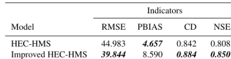
As summarized in Table 3, the RMSE of the improved model is 39.844 and it is lower than the original HEC-HMS RMSE (44.983), which means the outputs are closer to the observed data. The PBIAS (4.657) of the original model is closer to zero than the improved HEC-HMS PBIAS (8.590), which means the improved method overestimates the obser-vations. The NSE and CD values (0.850 and 0.884) of the im-proved HMS are closer to one than the original HEC-HMS values (0.808 and 0.842), which means the improved model has a more acceptable level of performance and fits more to the observations. The smooth method, which is intro-duced in Sect. 2.3, cannot improve the results. This because there are not many spikes along the uphills and downhills.
As suggested by the statistical measurement comparisons in Table 4, the proposed method can also improve the uncal-ibrated HEC-HMS model. By inputting the same data, the RMSE is reduced from 134.610 to 89.882 by using 0.8 and 11 forαandλ, respectively. The time window is 1 week.
4 Discussion
As model driving forces, data input is heavily relied upon in physically based hydrologic models. On a physical ba-sis, the meteorologic input is modeled with water flow stor-age and paths within the earth system. The streamflow, as demonstrated in this research, is one example. During this process, all numerical models simplify physical processes to some degree, either spatial-wise, such as a hydrologic re-sponse unit, or temporal-wise, such as summer leaf index. Such conceptualization and simplification compose a static numerical modeling environment that cannot capture all en-vironmental stressors, such as in the meteorological inputs. These are long-term stressor issues in hydrologic science.
To capture environmental stressors, such as meteorolog-ical changing trends, land cover variation, and vegetation growth, we can use different hydrologic models or add
ad-method. The effect is similar to having multiple hydrologic models for different input data biases.
Machine learning in this application attempts to use rele-vant input data to reproduce hydrologic behavior, i.e., a flow hydrograph as close to observed as possible. The overall dif-ference in the observed and modeled hydrograph is catego-rized as an error. In hydrologic the literature, it has been rec-ognized that this difference can be due to uncertainty in input and output data, bias in model parameterization, and issues with model structure. With the current machine-learning ap-proaches, it is not possible to disentangle and attribute to-tal error to multiple sources such as input data, model pa-rameters, and model structure. Moreover, machine-learning approaches cannot provide physical reasoning for this error. This is a recognized issue in hydrology and an active area of research. Since no prior model structure is provided for the machine-learning approach – it learns model structure and parameters from input data and observed output – it can be stated that the contribution of model structure and parameters towards total error is relatively small compared to bias or un-certainty in model input. The separation of data into training and testing samples provides a safeguard against overfitting the model. However, issue of disentangling error and attribut-ing it to multiple sources remains unresolved in this work. Future research should focus on this issue.
processes; comparatively, as a representative of empirically based lumped-parameter hydrologic models, HEC-HMS is widely used for industrial engineering purposes, which con-ceptualize physical bases towards result-oriented simula-tions.
While implementing the pre-developed hydrologic simula-tion, the calibrated hydrologic models were “restored” to the original uncalibrated status for comparison purposes. Dur-ing the “restoration”, the calibrated parameters were adjusted to default values either from program manuals or authors’ personal suggestions. This may lead to a varying restoration status of uncalibrated model performance depending on the parameters suggested. However, in this study, the main goal for the development of uncalibrated hydrologic models is to compare model simulation and post-processing performance in a qualitative sense. Thus, the details of uncalibrated model development are not the main focus in the study.
There may be various types of default parameters used in a physical hydrologic model for development efficiency. Parameters can be classified as sensitive and insensitive or model execution related and process algorithm related. Apart from the model-execution-related parameters and other in-sensitive parameters, the process-algorithm-related sensi-tive parameters are typically critical to model development, which greatly affect the model’s performance. Default values can follow physical laws and be contained in the correspond-ing computation algorithms but not necessarily capture the regional hydrologic characteristics at a study site. Capturing such site-specific features is the process of calibration. As such, the differences between uncalibrated–default-set mod-els and calibrated modmod-els are determined by the significance of sensitive parameters affecting the modeling performance. A physical hydrologic model usually cannot generate good results with default values and requires calibration (Chen et al., 2015b; Hay et al., 2006; Hay and Umemoto, 2007b). In the paper, we have two examples showing that default values produce inaccurate results. With the same model and study area, the Table 1 calibrated original PRMS results are much more accurate than the Table 2 uncalibrated original PRMS based on performance evaluation indices. Similarly, the Ta-ble 3 calibrated original HEC-HMS results are much better than the Table 4 uncalibrated original HEC-HMS. Numeri-cal experiments have corroborated the superior performance
better fit with observations instead of overestimation, making the fitness evaluation in the PRMS model and post-processor more comparable.
5 Conclusion
In this paper, a post-processor framework is proposed to im-prove the accuracy of hydrologic models with a window size selection method embedded to solve the nonstationary con-cern in hydrologic data. The proposed post-processor frame-work leverages machine-learning approaches to character-ize the role that the model inputs play in the model predic-tion errors so as to improve hydrologic model predicpredic-tion re-sults. The proposed window size selection method enhances the performance of the proposed framework when dealing with nonstationary data. The results of two different hydro-logic models show that the accuracy of calibrated hydrohydro-logic models can be further improved; without calibration efforts, the results of uncalibrated hydrologic models using the pro-posed framework can be as accurate as the calibrated ones by leveraging the proposed framework, which means that our proposed methods are possibly able to ease the traditionally complex and time-consuming model calibration step.
Two case studies are introduced in this paper and we will examine the framework with other models and study fields. Also, it is interesting to study the peak values and better pre-diction algorithm for peak values in the future.
all the reviewers, especially Paul Miller for his constructive com-ments.
This material is based upon work supported by the National Sci-ence Foundation and the University of Nevada, Reno, Graduate Stu-dent Association Research Grant Program. Any opinions, findings, and conclusions or recommendations expressed in this material are those of the authors and do not necessarily reflect the views of the National Science Foundation.
Financial support. This research has been supported by the Na-tional Science Foundation (grant nos. IIA-1329469, IIA-1301726, IIS-1838024, EEC-1801727, and 173056).
Review statement. This paper was edited by Bethanna Jackson and reviewed by William Paul Miller and Bethanna Jackson.
References
Andreadis, K. and Lettenmaier, D.: Assimilating remotely sensed snow observations into a macroscale hydrology model, Adv. Wa-ter Resour., 29, 872–886, 2006.
Basak, D., Pal, S., and Patranabis, D. C.: Support vector regression, Neural Information Processing-Letters and Reviews, 11, 203– 224, 2007.
Bennett, T. H.: Development and Application of a Continuous Soil Moisture Accounting Algorithm for the Hydrologic Engineering Center Hydrologic Modeling System (HEC-HMS), Thesis MS, University of California, Davis, 1998.
Bennett, T. H. and Peters, J. C.: Continuous Soil Moisture Account-ing in the Hydrologic EngineerAccount-ing Center Hydrologic Model-ing System (HEC-HMS), World Environmental and Water Re-sources Congress, 8806, 1–10, 2004.
Bifet, A. and Gavalda, R.: Learning from time-changing data with adaptive windowing, in: Proceedings of the 2007 SIAM Interna-tional Conference on Data Mining, SIAM, 443–448, 2007. Bifet Figuerol, A. C. and Gavaldà Mestre, R.: Advances in
Intelli-gent Data Analysis VIII, IDA 2009, Lecture Notes in Computer Science, vol. 5772, Springer, Berlin, Heidelberg, 2009.
Bouchachia, A.: Fuzzy classification in dynamic environments, Soft Computing, 15, 1009–1022, 2011.
Breiman, L.: Random forests, Mach. Learn., 45, 5–32, 2001.
tributed Hydrological Modeling for a Snow Dominant Water-shed Using a Precipitation and Runoff Modeling System, in: World Environmental and Water Resources Congres, 2527– 2536, 2015a.
Chen, C., Fenstermaker, L., Stephen, H., and Ahmad, S.: Dis-tributed hydrological modeling for a snow dominant watershed using a precipitation and runoff modeling system, in World En-vironmental and Water Resources Congress 2015, 2527–2536, 2015b.
Chen, C., Ahmad, S., M. J., and Kalra, A.: Study of Lehman Creek Watershed’s Hydrologic Response to Climate Change Us-ing Downscaled CMIP5 Projections, World Environmental and Water Resources Congress 2016, 508–517, 2016.
Chen, C., Kalra, A., and Ahmad, S.: A Conceptualized Ground-water Flow Model Development for Integration with Surface Hydrology Model, World Environmental and Water Resources Congress, 175–187, 2017.
Domingos, P.: A few useful things to know about machine learning, Communications of the ACM, 55, 78–87, 2012.
Domingos, P. and Hulten, G.: Mining high-speed data streams, in: Proceedings of the sixth ACM SIGKDD international conference on Knowledge discovery and data mining, 71–80, ACM, 2000. Duan, Q., Sorooshian, S., and Gupta, V.: Effective and efficient
global optimization for conceptual rainfall-runoff models, Water Resour. Res., 28, 1015–1031, 1992.
Duan, Q., Sorooshian, S., and Gupta, V.: Optimal use of the SCE-UA global optimization method for calibrating watershed mod-els, J. Hydrol., 158, 265–284, 1994.
Duan, Q., Schaake, J., Andreassian, V., Franks, S., Goteti, G., Gupta, H., Gusev, Y., Habets, F., Hall, A., Hay, L., and Hogue, T.: Model Parameter Estimation Experiment (MOPEX): An overview of science strategy and major results from the second and third workshops, J. Hydrol., 320, 3–17, 2006.
Environmental Protection Agency: Environmental Model-ing | US EPA, available at: https://www.epa.gov/aboutepa/ about-office-policy-op (last access: 9 April 2018), 2017. Friedman, J.: On bias, variance, 0/1-loss, and the
curse-of-dimensionality, Data Min. Knowl. Disc., 1, 55–77, 1997. Gama, J., Medas, P., Castillo, G., and Rodrigues, P.: Learning with
drift detection, in: Brazilian Symposium on Artificial Intelli-gence, 286–295, Springer, 2004.
Georgia Watersheds: Agricultural Research Service Hydrology Laboratory, available at: https://hrsl.ba.ars.usda.gov/wdc/ga.htm (last access: 20 August 2019), 2007.
Hay, L. E. and Umemoto, M.: Multiple-objective stepwise calibra-tion using Luca, US Geological Survey, p. 25, 2007b.
Hay, L. E., Leavesley, G. H., Clark, M. P., Markstrom, S. L., Viger, R. J., and Umemoto, M.: Step wise, multiple objective calibration of a hydrologic model for a snowmelt dominated basin 1, J. Am. Water Resour. As., 42, 877–890, 2006.
Huang, N. E., Shen, Z., Long, S. R., Wu, M. C., Shih, H. H., Zheng, Q., Yen, N.-C., Tung, C. C., and Liu, H. H.: The empirical mode decomposition and the Hilbert spectrum for nonlinear and non-stationary time series analysis, Proc. R. Soc. Lond. A Mat., 454, 903–995, 1998.
Klinkenberg, R. and Joachims, T.: Detecting Concept Drift with Support Vector Machines, ICML, 487–494, 2000.
Klinkenberg, R. and Renz, I.: Adaptive information filtering: Learn-ing in the presence of concept drifts, LearnLearn-ing for Text Catego-rization, 33–40, 1998.
Kohavi, R.: A study of cross-validation and bootstrap for accuracy estimation and model selection, Ijcai, 14, 1137–1145, Stanford, CA, 1995.
Krzysztofowicz, R. and Maranzano, C.: Bayesian system for proba-bilistic stage transition forecasting, J. Hydrol., 299, 15–44, 2004. Lanquillon, C.: Enhancing text classification to improve informa-tion filtering, PhD thesis, Otto-von-Guericke-Universität Magde-burg, Universitätsbibliothek, 2001.
Leavesley, G. H., Lichty, R. W., Troutman, B. M., and Saindon, L. G.: Precipitaion-Runoff Modeling System:User’s manual, Water-Resources Investigations Report, 83–4238, 1983.
Liu, Y., Wang, W., Hu, Y., and Cui, W.: Improving the Distributed Hydrological Model Performance in Upper Huai River Basin: Using Streamflow Observations to Update the Basin States via the Ensemble Kalman Filter, Adv. Meteorol., 61, 1–14, 2016. Madadgar, S., Moradkhani, H., and Garen, D.: Towards improved
post-processing of hydrologic forecast ensembles, Hydrol. Pro-cess., 28, 104–122, 2014.
Markstrom, S. L.and Niswonger, R. G., Regan, R. S., Prudic, D. E., and Barlow, P. M.: GSFLOW – Coupled Ground-Water and Surface-Water Flow Model Based on the Integration of the Precipitation-Runoff Modeling System (PRMS) and the Modu-lar Ground-Water Flow Model, Water-Resources Investigations Report, 2005.
Markstrom, S. L., Regan, S., Hay, L. E., Viger, R. J., Webb, R. M. T., Payn, R. A., and LaFontaine, J. H.: the Precipitation-Runoff Modeling System, Version 4, U.S. Geological Survey Techniques and Methods, Book 6, chap. B7, Clarendon Press, https://doi.org/10.3133/tm6B7, 2015.
Montanari, A. and Brath, A.: A stochastic approach for assess-ing the uncertainty of rainfall-runoff simulations, Water Resour.
Safari, A. and De Smedt, F.: Improving the Confidence in Hy-drologic Model Calibration and Prediction by Transforma-tion of Model Residuals, J. Hydrol. Eng., 20, 04015001, https://doi.org/10.1061/(ASCE)HE.1943-5584.0001141, 2015. Scharffenberg, W. and Fleming, M.: Hydrologic modeling system
HEC-HMS: user’s manual, US Army Corps of Engineers, Hy-drologic Engineering Center, 2006.
Schweppe, F.: Uncertain dynamic systems, Prentice-Hall, 1973. Seo, D.-J., Herr, H. D., and Schaake, J. C.: A statistical
post-processor for accounting of hydrologic uncertainty in short-range ensemble streamflow prediction, Hydrol. Earth Syst. Sci. Dis-cuss., 3, 1987–2035, https://doi.org/10.5194/hessd-3-1987-2006, 2006.
Skahill, B., Baggett, J., Frankenstein, S., and Downer, C.: More ef-ficient PEST compatible model independent model calibration, Environ. Modell. Softw., 24, 517–529, 2009.
Slater, A. and Clark, M.: Snow data assimilation via an ensemble Kalman filter, J. Hydrometeorol., 7, 478–493, 2006.
Srivastava, A., Rajeevan, M., and Kshirsagar, S.: Development of a high resolution daily gridded temperature data set (1969–2005) for the Indian region, Atmos. Sci. Lett., 10, 249–254, 2009. US Army Corps of Engineers: HEC-HMS Downloads, available at:
https://www.hec.usace.army.mil/software/hec-hms/downloads. aspx, last access: 19 August 2019.
USDA: Agricultural Research Service Hydrology Labora-tory, available at: https://www.ars.usda.gov/northeast-area/ beltsville-md-barc/beltsville-agricultural-research-center/ hydrology-and-remote-sensing-laboratory/docs/rsbasics/ research/ (last access: 21 August 2019), 1997.
USGS: USGS.gov| Science for a changing world, available at: https://www.usgs.gov/, last access: 21 August 2017.
USGS: Precipitation Runoff Modeling System (PRMS), available at: https://www.usgs.gov/software/ precipitation-runoff-modeling-system-prms, last access: 19 August 2019.
Volk, J. M.: Potential Effects of a Warming Climate on Water Re-sources within the Lehman and Baker Creek Drainages, Great Basin National Park, Nevada, 2014.
Wang, Q., Shrestha, D., Robertson, D., and Pokhrel, P.: An analysis of transformations, J. R. Stat. Soc. Ser. B Met., 211–252, 1964. Wang, Q., Shrestha, D., Robertson, D., and Pokhrel, P.:
A log-sinh transformation for data normalization and variance stabilization, Water Resour. Res., 48, W05514, https://doi.org/10.1029/2011WR010973, 2012.