Bayesian inference and predictive performance of soil respiration
models in the presence of model discrepancy
Ahmed S. Elshall1,2, Ming Ye3, Guo-Yue Niu4,5, and Greg A. Barron-Gafford4,6 1Department of Earth Sciences, University of Hawai‘i at M¯anoa, Honolulu, Hawaii, USA 2Water Resources Research Center, University of Hawai‘i at M¯anoa, Honolulu, Hawaii, USA
3Department of Earth, Ocean, and Atmospheric Science, Florida State University, Tallahassee, Florida, USA 4Biosphere 2, University of Arizona, Tucson, Arizona, USA
5Department of Hydrology and Water Resources, University of Arizona, Tucson, Arizona, USA 6School of Geography and Development, University of Arizona, Tucson, Arizona, USA Correspondence:Ming Ye ([email protected])
Received: 31 October 2018 – Discussion started: 26 November 2018
Revised: 16 April 2019 – Accepted: 23 April 2019 – Published: 23 May 2019
Abstract. Bayesian inference of microbial soil respiration models is often based on the assumptions that the residu-als are independent (i.e., no temporal or spatial correlation), identically distributed (i.e., Gaussian noise), and have con-stant variance (i.e., homoscedastic). In the presence of model discrepancy, as no model is perfect, this study shows that these assumptions are generally invalid in soil respiration modeling such that residuals have high temporal correlation, an increasing variance with increasing magnitude of CO2 ef-flux, and non-Gaussian distribution. Relaxing these three as-sumptions stepwise results in eight data models. Data models are the basis of formulating likelihood functions of Bayesian inference. This study presents a systematic and comprehen-sive investigation of the impacts of data model selection on Bayesian inference and predictive performance. We use three mechanistic soil respiration models with different levels of model fidelity (i.e., model discrepancy) with respect to the number of carbon pools and the explicit representations of soil moisture controls on carbon degradation; therefore, we have different levels of model complexity with respect to the number of model parameters. The study shows that data models have substantial impacts on Bayesian inference and predictive performance of the soil respiration models such that the following points are true: (i) the level of complexity of the best model is generally justified by the cross-validation results for different data models; (ii) not accounting for het-eroscedasticity and autocorrelation might not necessarily re-sult in biased parameter estimates or predictions, but will
def-initely underestimate uncertainty; (iii) using a non-Gaussian data model improves the parameter estimates and the pre-dictive performance; and (iv) accounting for autocorrelation only or joint inversion of correlation and heteroscedasticity can be problematic and requires special treatment. Although the conclusions of this study are empirical, the analysis may provide insights for selecting appropriate data models for soil respiration modeling.
1 Introduction
tool for the model–data integration (Luo et al., 2011, 2014; Wieder et al., 2015). In addition, use of state-of-the-art statis-tical methods is necessary to accurately quantify uncertainty in parameters and structures of soil respiration models for the improvement and practical use of the models (Katz et al., 2013). A data model, also known as a residuals model or an error model, is used to characterize residuals (i.e., the dif-ference between data and corresponding model simulations). While a large number of data models have been used (e.g., Elshall et al., 2018; Scholz et al., 2018), to our knowledge, a comprehensive and systematic evaluation of data models for soil respiration modeling has not been reported in the litera-ture.
The objectives of this study are to evaluate the impacts of data models on Bayesian inference and predictive perfor-mance of three mechanistic soil respiration models, and to use the evaluation results to make broader recommendations. The three models were developed by Zhang et al. (2014) to simulate the Birch effect (the peak soil microbial respi-ration pulses in response to episodic rainfall pulses) at the site scale and at a short temporal scale; understanding the Birch effect is important to gain a mechanistic understanding of CO2efflux production (Högberg and Read, 2006; Vargas et al., 2011). The models from Zhang et al. (2014) are based on an existing four-carbon-pool model from Allison et al. (2010), but have additional carbon pools and/or explicit rep-resentations of soil moisture controls on carbon degradation and microbial uptake rates. The models were calibrated, and Bayesian model selection was used to select the best model (Zhang et al., 2014). However, this effort was based on a sin-gle data model. It is unknown whether the best model still remains the best (in terms of reproducing both the calibration data and the cross-validation data) if a different data model is used. In addition, as predictive performance of the mod-els was not evaluated in Zhang et al. (2014), it is unknown if the best model will give the best predictions. These two questions are addressed in this study by considering eight data models and by evaluating predictive performance us-ing cross-validation. The top two models (also the two most high-fidelity models) ranked by Zhang et al. (2014) are con-sidered in this study, and the worst model (also the low-fidelity model) is also considered for comparison. We use the terms model fidelity and model discrepancy interchangeably. Model fidelity refers to the degree of realism of the model regarding representing our scientific knowledge with respect to the real world system; hence a high-fidelity model has less discrepancy. Evaluating predictive performance for the three models with different degrees of fidelity provides more in-sights than a single model.
Bayesian inference in general uses the Bayes’ theorem to update the prior distributions of model parameters to posterior parameter distributions given a likelihood func-tion of data. The mathematical formulafunc-tion of the (for-mal and infor(for-mal) likelihood function requires a probabilis-tic data model; however, this probability model is
intrinsi-cally unknown due to unknown errors in all model com-ponents such as model structures, parameters, and driving forces. Bayesian inference of soil respiration models often adopts the assumption of independent, normally distributed, and homoscedastic residuals (e.g., Ahrens et al., 2014; Bag-nara et al., 2015, 2018; Barr et al., 2013; Barron-Gafford et al., 2014; Braakhekke et al., 2014; Braswell et al., 2015; Cor-reia et al., 2012; Du et al., 2015, 2017; Hararuk et al., 2014; Hashimoto et al., 2011; He et al., 2018; Keenan et al., 2012; Klemedtsson et al., 2008; Menichetti et al., 2016; Raich et al., 2002; Ren et al., 2013; Richardson and Hollinger, 2005; Steinacher and Joos, 2016; Tucker et al., 2014; Tuomi et al., 2008; Xu et al., 2006; Yeluripati et al., 2009; Yuan et al., 2012, 2016; Zhang et al., 2014; Zhou et al., 2010). These assumptions are conveniently adopted to satisfy the require-ment of using an unknown probability model in Bayesian statistics, which was referred to as “a basic dilemma” by Box and Tiao (1992).
Postulating the data models is always based on assump-tions about residual statistics, and the most widely used as-sumptions are paired as follows: (i) independent vs. corre-lated residuals, (ii) homoscedastic vs. heteroscedastic resid-uals, and (iii) Gaussian vs. non-Gaussian residuals. For soil respiration modeling few studies have relaxed the non-correlation assumption (e.g., Cable et al., 2008, 2011; Q. Li et al., 2016), the homoscedasticity assumption (e.g., Berry-man et al., 2018; Elshall et al., 2018; Ogle et al., 2016; Tucker et al., 2013), and the non-Gaussian and homoscedasticity as-sumptions (e.g., Elshall et al., 2018; Ishikura et al., 2017; Kim et al., 2014). A recent study by Scholz et al. (2018) relaxed these three assumptions using the generalized like-lihood function developed by Schoups and Vrugt (2010). However, few studies have focused on investigating the ap-propriateness and impact of these assumptions for soil res-piration modeling by relaxing the independent residuals as-sumption (Ricciuto et al., 2011) and the Gaussian residuals assumption (Ricciuto et al., 2011; van Wijk et al., 2008). By relaxing these three assumptions stepwise, to our knowledge this is the first study that systematically evaluates the impact of data model selection on Bayesian inference and predic-tive performance of soil respiration modeling. In addition, to our knowledge, this is the first soil respiration modeling study that investigates the impact of data models in relation to model fidelity.
assump-(McInerney et al., 2017; T. Smith et al., 2010, 2015) is neces-sary to evaluate the appropriateness of residuals assumptions and their impacts on Bayesian inference.
The assumptions of heteroscedastic, correlated, and non-Gaussian residuals are accounted for using the method of Schoups and Vrugt (2010) in the following procedure: (i) the correlation is removed from the residuals using an autore-gressive model; (ii) the resulting residuals are normalized by a linear model of variance; and (iii) the normalized residuals are characterized using the skew exponential power distribu-tion. The data model parameters (i.e., coefficients of the au-toregressive model, the linear variance model, and the skew exponential power distribution) are not specified by users, but are estimated along with the soil respiration model pa-rameters during the Bayesian inference. The skew exponen-tial power distribution is general in that by adjusting the val-ues of its kurtosis and skewness parameters the distribution can produce distributions such as the Laplace distribution (van Wijk et al., 2008; Ricciuto et al., 2011) or the distri-butions from the study by Tang and Zhuang (2009), which utilized an exponential model with different kurtosis param-eters. It is worth pointing out that other methods exist to account for the three assumptions. Evin et al. (2013) sug-gested accounting for residual heteroscedasticity before ac-counting for residual autocorrelation. Lu et al. (2013) devel-oped an iterative two-stage procedure to separately estimate physical model parameters and data model parameters. Evin et al. (2014) developed a similar procedure to first estimate model parameters and then estimate heteroscedasticity and autocorrelation parameters. While this study uses the method from Schoups and Vrugt (2010), exploring other methods is warranted in future studies.
After investigating the impacts of the data models on Bayesian inference, this study evaluates the impacts of the data models on the predictive performance of the three soil respiration models. Using random samples generated during the Bayesian inference, a prediction ensemble is produced for each soil respiration model. The ensemble is used to eval-uate predictive performance of the models in a stochastic sense by estimating extent to which the models can predict future events. The evaluation in this study is carried out us-ing cross-validation by splittus-ing the CO2efflux dataset into two parts for Bayesian inference and cross-validation, re-spectively. The evaluation of predictive performance is im-portant because different data models may give different pa-rameter distributions and therefore different predictive per-formance. For example, the study by van Wijk et al. (2008)
evaluation of predictive analysis is conducted for the fol-lowing two cases: (1) the prediction ensemble is generated by random samples of the soil respiration models only (i.e., credible interval), and (2) the prediction ensemble is gener-ated by random samples of not only the soil respiration mod-els but also the data modmod-els (i.e., predictive interval). The two cases lead to different conclusions about the predictive performance. It is expected that the evaluation of predictive performance conducted in this study can help select the most appropriate data model to achieve optimal model predictions. The remainder of the paper is organized as follows. Sec-tion 2 starts with a descripSec-tion of the evolving data mod-els and their corresponding likelihood functions used in Bayesian inference, followed by a brief summary of the three soil respiration models. The results of Bayesian inference are discussed in Sects. 3 and 4, addressing the data model impli-cations on parameter estimation and predictive performance, respectively. Section 5 summarizes the key findings and lim-itations of this study, and provides recommendations for ap-proaching data model selection.
2 Methodology
This section starts with a description of the eight data models that account for the three pairs of assumptions about residu-als in a stepwise manner in Sect. 2.1. The data models are used to build the likelihood functions used in Sect. 2.2 for Bayesian inference. The three soil respiration models and ob-servations of CO2efflux are described in Sect. 2.3 and 2.4, respectively. Metrics for evaluating predictive performance are presented in Sect. 2.5.
2.1 Data models
This study considers eight evolving data models starting from a data model that assumes independent, homoscedas-tic, and Gaussian residuals to a data model that relaxes all three assumptions. The eight data models are based on the generic normalized residual,
at= εt σt
at∼X, (1)
models are formulated with different forms ofεt,σt, andX. The standard least square (SLS) data model is
at= εt σ0
at∼N (0,1), (2)
where σt=σ0 is a constant for all of the data (i.e., ho-moscedasticity), and X is the standard normal distribution,
N (0,1). The unknown parameterσ0is estimated along with the unknown physical model parameters. Ifσt is not a con-stant (i.e., heteroscedastic), SLS becomes the weighted least squared (WLS) data model. While heteroscedasticity can be accounted for via residuals transformation (e.g., Thiemann et al., 200; T. Smith et al., 2010) or other similar approaches (Gragne et al., 2015), a linear heteroscedastic model σt= σ0+σ1Yt is assumed here following the studies of Thyer et al. (2009), Schoups and Vrugt (2010), and Evin et al. (2013, 2014). With the linear model, there is no need to estimateσt for each piece of data. Instead,σt is calculated by estimat-ing only two parameters,σ0andσ1. The WSL data model is written as
at= εt σ0+σ1Yt
at ∼N (0,1). (3)
The two unknown parametersσ0andσ1are estimated along with the unknown physical model parameters. The linear model assigns smaller weights to data with larger simulation values,Yt. If the simulation value is small andσ0σ1Yt, the weight becomes constant for all data. Both SLS and WLS as-sume thatat is independently and identically distributed.
It is not uncommon that residuals are correlated in space and time, due to the propagation of measurement errors (Tiedeman and Green, 2013) and model structure errors (Evin et al., 2014; Kavetski et al., 2003; Lu et al., 2013). The temporal correlation that occurs in the numerical example of this study can be accounted for by using a p order autore-gressive model. This leads to the standard least square data model with autocorrelation (SLS-AC):
at= εt−
p P
i=1
φiεt−i
σ0
at∼N (0,1), (4)
wherep is the order of autocorrelation, and φi is an auto-correlation coefficient. The unknownφiandσ0are estimated along with the unknown model parameters. Extending the concept of correlated residuals to WLS leads to the weighted least squared with autocorrelation (WLS-AC):
at= εt−
p P
i=1
φiεt−1
σ0+σ1Yt
at∼N (0,1). (5)
The unknown parameters of σ0, σ1, and φi are estimated along with the physical model parameters. Equations (2)–(5) assume that the residuals are Gaussian.
The next four data models are similar to the previous four models except that the standard normal distribution of
at is replaced by the skew exponential power distribution, SEP(0,1, ξ, β), with a zero mean and unit standard devia-tion (Schoups and Vrugt, 2010):
p (at|ξ, β)= 2σξ
ξ+ξ−1ωβexp h
−cβ aξ,t
2/(1+β)i
, (6)
where ξ is skewness, β is kurtosis, aξ, t= µξ+σξat ξsign(µξ+σξat), µξ=M ξ−ξ−1, ωβ=
01/2[3(1+β)/2]
(1+β)03/2[(1+β)/2], σξ = q
1−M2
ζ2+ζ−2
+2M2−1,
M= 0[1+β]
01/2[3(1+β)/2]01/2[(1+β)/2], and cβ= 0[3(1+β)/2]
0[(1+β)/2]
1/(1+β)
are derived variables of β and ξ, and 0[.] is the gamma function. The kurtosis parameter {β∈R: −1≤β≤1} determines the peakedness of the PDF such that theβ values of−1, 0, and 1 give uniform, Gaussian, and Laplace distributions, respectively. The skewness parameter {ξ∈R:0.1≤ξ≤10} determines the skewness of the PDF such that the ξ values of 0.1, 1, and 10 give positively skewed, symmetric, and negatively skewed distributions, respectively. Settingβ=0 andξ =1 leads to µξ=0, σξ=1, ωβ=1
.√
2π, cβ=12 , and aξ, t=at, and the skew exponential power distribution SEP(0,1, ξ=1, β=0) becomes the standard normal distribution,
p (at|ξ =1, β=0)= 1 √
2πexp
−1 2(at)
2
, (7)
which is the SLS data model in Eq. (2).
Replacing at ∼N (0,1) with at∼SEP(0,1, ξ, β) in Eqs. (2)–(4) leads to the SEP, WSEP, SEP-AC, and WSEP-AC data models as follows:
at= εt
σ0
at∼SEP(0,1, ξ, β) (8)
at= εt σ0+σ1Yt
at∼SEP(0,1, ξ, β) . (9)
at= εt−
p P
i=1
φiεt−1
σ0
at∼SEP(0,1, ξ, β) (10)
at= εt−
p P
i=1
φiεt−1
σ0+σ1Yt
at∼SEP(0,1, ξ, β) (11)
distributions,p(θ|d), of model parameters,θ, given data,d, using Bayes’ theorem (Box and Tiao, 1992):
p (θ|d)=R p (d|θ) p (θ)
p (d|θ) p (θ)dθ, (12)
wherep(θ)is the prior distribution, andp(d|θ)is the like-lihood function to measure goodness-of-fit between model simulations,Y (θ), and data,d. The prior distribution can be obtained using data from previous studies (e.g., Elshall and Tsai, 2014) or expert judgment. When prior information is lacking, a common practice is to assume uniform distribu-tions with relatively large parameter ranges so that the prior distributions do not affect the estimation of posterior distri-butions.
The data models above can be used to construct the like-lihood functions. For the Gaussian data models given in Eqs. (2)–(5), the corresponding Gaussian likelihood func-tions are straightforward (see Eq. 7 for an example). For the SEP data models, the corresponding likelihood, which is called generalized likelihood function, is (Schoups and Vrugt, 2010)
p (d|θ)=p (εt|θ)
= n Y
t=1
σt−1 2σξ
ξ+ξ−1ωβexp
−cβ aξ, t
2/(1+β)
, (13)
wherenis the dimension ofd. The Gaussian likelihood tions are special cases of the generalized likelihood func-tions. For example, by settingβ=0,ξ =1,φi =0,σt=σ0, σξ =1, µξ =0, ωβ=1
.√
2π, cβ=12 , and aξ, t=at, Eq. (13) becomes the likelihood function corresponding to the SLS data model. Replacing σt =σ0byσt=σ0+σ1Et, Eq. (13) becomes the likelihood function of the WLS data model.
In this study, the posterior distributions of the data model parameters are estimated along with the soil respiration model parameters using the MT-DREAM(ZS) code (Laloy and Vrugt, 2012). MT-DREAM(ZS) implements a Markov chain Monte Carlo (MCMC) algorithm by running multiple Markov chains in parallel with adaptive proposal distribu-tion, multiple-try sampling, and sampling from an archive of past states. These state-of-the-art features assist in overcom-ing common challenges in the samplovercom-ing space such as multi-modality, ill-conditioning, and high dimensionality, and thus allow for accurate exploration of the targeted distributions.
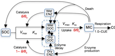
the five models are used in this study, and they are denoted as 4C, 5C, and 6C. Note that model 4C is model 4C_NOSM from Zhang et al. (2014), not their model 4C. Figure 1 is the diagram of model 6C, the most complex of the five models. The simplest model, model 4C, has four carbon pools, i.e., soil organic carbon (SOC), dissolved organic carbon (DOC), microbial biomass (MIC), and enzymes (ENZ), and does not consider the soil moisture control on carbon degradation and microbial uptake rates. Models 5C and 6C have an explicit representation of soil moisture controls on the rates. Based on the dual Arrhenius and Michaelis–Menten kinetics model, the original SOC degradation rate,Vdecom, is (Davidson et al., 2011; Davidson and Janssens, 2006)
Vdecom=VmaxCENZ
CSOC
Km+CSOC
, (14)
where Vmax (s−1) is the maximum SOC degradation rate per unit enzyme when the substrates is not limiting,CENZ (g C m−3) is enzyme pool size,CSOC(g C m−3) is SOC pool size, andKmis the half-saturation for SOC. The original mi-crobial uptake rate,Vuptake, is (Davidson et al., 2011; David-son and Janssens, 2006)
Vuptake=Vmax_upCMIC
CDOC
Km_up+CDOC
CO2 Km_upO2+CO2
, (15)
whereVmax_up(s−1) is the maximum DOC uptake rate when the substrates is not limiting,CMIC(g C m−3) is the MIC pool size,CDOC (g C m−3) is the DOC pool size,CO2 (m
3m−3) is the gas concentration of O2 in the soil pore, and Km_up (g C m−3) andKm_upO2(m
3m−3) are the corresponding half-saturation constants for DOC and O2, respectively. With the explicit representation of soil moisture control, the two rates become (Zhang et al., 2014)
Vdecom=VmaxCENZ
CSOC
Km+CSOC θ
θs
(16)
Vuptake=Vmax_upCMIC
CDOC
Km_up+CDOC
CO2 Km_upO2+CO2
θ
θs
, (17)
whereθ (–) is the volumetric soil moisture, andθs(–) is the porosity.
Figure 1. Diagram of model 6C representing the processes of (1) degradation of soil organic carbon (SOC) to dissolved organic carbon (DOC) through the catalysis of enzymes (ENZ) produced by microbes (MIC), (2) MIC uptake of DOC, and (3) microbial (MIC) respiration to produce CO2(CUE is the carbon use efficiency). SOC degradation and microbial uptake rates are controlled by water satu-ration(θ/θs). The DOC and ENZ pools are split into two sub-pools, one for the wet zone and the other for the dry zone of the soil pore space. Microbial uptake of DOC only occurs in the wet zone, and the uptake rate is linearly related toθ/θs. Catalysis through ENZ in the wet zone is proportional toθ/θs, whereas that in the dry zone is proportional to 1−θ/θs.Vmax(s−1) is the maximum rate, andKm is the half-saturation concentration.
and only the wet DOC is used by MIC, as shown in Fig. 1. The moisture-controlled microbial uptake rate becomes
Vuptake=Vmax_upCMIC
CDOC_W
Km_up+CDOC_W
CO2 Km_upO2+CO2
θ
θs
, (18)
whereCDOC_W(g C m−3) is the DOC pool size in the wet soil pores. Model 6C is more complex in that ENZ is further split into two sub-pools for wet and dry pores, and both the wet and dry ENZ are subject to degradation, as shown in Fig. 1. The moisture-controlled SOC degradation rate becomes
Vdecom=VmaxCENZ_W
CSOC
Km+CSOC θ
θs
(19) for the wet ENZ and
Vdecom=VmaxCENZ_D
CSOC
Km+CSOC
1− θ
θs
εD (20)
for the dry ENZ, where CENZ_W (g C m−3) is the wet soil pores enzyme pool size, CENZ_D (g C m−3) is the enzyme pool size in the dry soil pores, and εD is the catalysis effi-ciency of the dry zone enzyme.
Due to considering the moisture control and adding more soil pools, model 5C is expected to be significantly better than model 4C for simulating the Birch effect. As the accu-mulated ENZ in dry soil is secondary, model 6C is expected to be slightly better than model 5C. In terms of model struc-tural error, model 4C has the largest model structure error,
model 5C has significantly less model structure error, and model 6C has the smallest model structural error. In other words, model 6C has the highest model fidelity (i.e., low-est model discrepancy) among the three models. As shown below, the degree of model structural error is reflected in the process of Bayesian inference and verified by the cross-validation.
2.4 Observations and parameter estimation
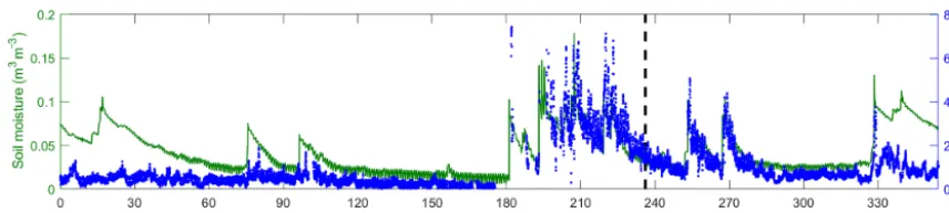
Figure 2 plots the time series of 17 016 observations of soil moisture and CO2 efflux used in this study. The observa-tions were obtained during the entire year of 2007, cover-ing a long period of dry season prior to the monsoon and episodic rainfall events during the monsoon. The first two-thirds of this dataset are used for the Bayesian inference, and the last third is used for cross-validation. The inference and cross-validation periods have both dry and wet periods, as shown in Fig. 2. The observation site is located within the Santa Rita Experimental Range (SRER; 31.8214◦N, 110.8661◦W, elevation 1116 m) outside of Tucson, Arizona (Barron-Gafford et al., 2011; Scott et al., 2009). This sa-vanna site was covered by 22 % perennial grass, forbs, and subshrubs and 35 % mesquite. The soils are uniformly com-prised of Comoro loamy sand (77.6 % sand, 11.0 % clay, and 11.4 % silt). The half-hourly atmospheric forcing data were collected from measurements via an eddy covariance tower (Scott et al., 2009). This includes downward shortwave ra-diation, longwave rara-diation, precipitation, wind, air tempera-ture, humidity, and pressure. The volumetric CO2 concentra-tion was measured at a half-hourly intervals using compact probes. The CO2efflux was estimated from the gradient of the CO2concentration measured at two depths (2 and 10 cm) using Fick’s first law of diffusion, and the estimates were validated against measurements from a portable CO2gas an-alyzer.
The parameters estimated in this study include the param-eters of the soil respiration models (4C–6C) and the parame-ters of the data models described in Sect. 2.1. The estimated parameters of models 4C and 5C include the microbial car-bon use efficiency (CUE) (g g−1), enzyme production rate,
ke(g m−3s−1), microbial turnover rate,τm (1 s−1), and en-zyme turnover rateτe(1 s−1). Uniform distributions are used as the prior in the Bayesian inference, and the ranges of the four parameters are 0.2–1.00, 1×10⁻¹²–1×10⁻⁷, 1×10⁻¹²– 1×10⁻⁵, and 1×10⁻¹¹–1×10⁻⁶, respectively. The values of other parameters are fixed at the values used in Allison et al. (2010). Model 6C has two more parameters, and they are the catalysis efficiencyεD(–) and the turnover rate of the dry-zone enzymesτen(1 s−1). The priors of the two parame-ters are uniform distributions with the ranges of 0.2–0.8 and 1×10⁻¹²–1×10⁻⁸, respectively.
parame-Figure 2.Time series of soil moisture and efflux observations. The dashed line marks the divide of the dataset into calibration and validation periods.
ter distributions are obtained after drawing a total of 5×10⁵ samples using five Markov chains. The Gelman and Rubin (1992) R statistic is used for the convergence diagnostic, and it approaches 1 in less than 40 000 samples. The initial 50 % of the samples are discarded during the burn-in period. 2.5 Metrics for evaluating predictive performance Three criteria are used to evaluate the predictive performance of the soil respiration models and data models: the central mean tendency, the dispersion, and the reliability. Each cri-terion is measured by a single metric. In addition, a newly defined metric by Elshall et al. (2018) is also used to simul-taneously measure the three criteria.
The central mean tendency is measured in this study us-ing the Nash–Sutcliffe model efficiency (NSME) coefficient (Nash and Sutcliffe, 1970),
NSME=1− n X
i=1
di−Yi 2
, n
X
i=1
di−d 2
, (21)
wherenis the number of cross-validation data,di is theith data,dis the mean of the data, andYi is the mean of the pre-diction ensemble,Yi, fordi. The NSME ranges from−∞to 1, with NSME=1 corresponding to a perfect match between data and mean prediction, i.e., the ensemble is centered on the data. NSME=0 indicates that the model predictions are only as accurate as the mean of the data, whereas an effi-ciency NSME<1 indicates that the mean of data is a better prediction than the mean prediction.
In addition to the central mean tendency, it is also desirable that the ensemble is precise, with small dispersion, and reli-able to cover all of the data. This study uses a nonparametric metric for dispersion, which is the sharpness of a prediction interval (e.g., M. W. Smith et al., 2010):
Sharpness=1 /nXn
i=1[Max(Yi)−Min(Yi)], (22) whereYi is the prediction ensemble within the 95 % predic-tion interval, the Bayesian credible interval, not the confi-dence interval used in nonlinear regression (Lu et al., 2013). Smaller sharpness values indicate better prediction precision. Reliability is measured using predictive coverage (e.g., Hoet-ing et al., 1999), which is the percentage of data contained in
the prediction interval. Larger predictive coverage values are preferred.
To account for the trade-off between the three metrics, Elshall et al. (2018) defined relative model score (RMS) that simultaneously measures all three criteria. Scoring rules are commonly used in hydrology to assess predictive perfor-mance (e.g., Weijs et al., 2010; Westerberg et al., 2011). The RMS is used in this study to measure the relative predictive performance of the combinations of soil respiration models and data models. For combinationMj, RMS is defined as
RMS Mj
= n X
i=1
p di|Yij, Mj m
P
j=1
p di|Yij, Mj
×100, (23)
wheremis the number of combinations; the ensemble pre-dictionYij is similar toYi above with indexiover time and indexj specific to thejth combination. The density func-tionp di|Yijcan be evaluated by first obtaining the den-sity function p Yij of the ensemble prediction Yij (e.g., by using the kernel density function) and then evaluating
p di|Yij using interpolation methods based on the inter-section of Yij anddi. More details about evaluating RMS can be found in Elshall et al. (2018). This evaluation is based purely on the model predictions, and does not involve any as-sumptions on the models, their parameters, or their likelihood functions. Larger RMS values indicate better overall predic-tive performance. A figure displaying our workflow scheme is presented in the Supplement.
3 Results of Bayesian inverse modeling
This section analyzes the residuals of the best realization (with the highest likelihood value) of the MCMC simula-tion to understand whether the assumpsimula-tions of the eight data models hold. The impacts of the data models on the posterior parameter distributions are also analyzed.
3.1 Residual characterization
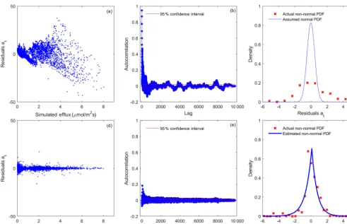
Figure 3.Residual analysis of the best realization (among multiple MCMC realizations) for model 6C using the(a–c)SLS and(d–f) WSEP-AC data models.
model with the assumptions of homoscedastic, independent, and Gaussian residuals, and WSEP-AC is the most complex model without the assumptions. Model 6C is the most com-plex model and also the best model as ranked by Zhang et al. (2014) using Bayesian model selection. The variable at, plotted in Fig. 3a–c and Fig. 3d–f, is defined in Eqs. (2) and (11), respectively. Figure 3a–c show that all three resid-ual assumptions are violated when SLS is used, as (i) the residual variance is not constant, but increases as a function of the simulated CO2efflux (Fig. 3a); (ii) the autocorrelation function at most lags is beyond the 95 % confidence inter-val (Fig. 3b); and (iii) the standard normal density function cannot adequately characterize the residuals (Fig. 3c). Fig-ure 3d–f show that, after relaxing the three assumptions, the processed residuals,at, can be well characterized by WSEP-AC. Figure 3d shows that, after normalizingεtwith the linear variance (σt=0.034+0.099Et), the variation of the variance ofat becomes significantly smaller, although the variance is still not constant. Figure 3e shows that, after removing a first-order autoregressive model from εt,at becomes less corre-lated, although the correlation is not fully removed. The two coefficients of the autoregressive model areφ1=0.989 and
φ2=4.5×10⁻⁶; the small value ofφ2indicates that there is no need to attempt an autoregressive model of higher order.
Figure 3f shows thatatfollows the SEP distribution with the estimated skewness coefficient ofξ =0.933 and kurtosis co-efficient ofβ=0.998. As a summary, Fig. 3 shows that it is important to examine the residuals and to determine whether the selected data model is adequate for characterizing the residuals. While WSEP-AC still cannot perfectly character-izeεt, it is significantly better than SLS.
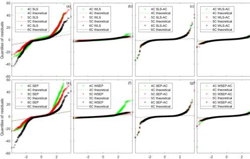
Figure 4.Residual quantile–quantile (Q–Q) plots of the best realization (among multiple MCMC realizations) for the three soil respiration models and eight data models.
indication of outliers (Thyer et al., 2009). The deviation is reduced after accounting for autocorrelation in SLS-AC and SEP-AC, as shown in Fig. 4c and g. It is interesting to ob-serve from the two figures that the Q–Q plots of the three models are visually almost identical. The deviation is almost fully removed after accounting for heteroscedasticity in WLS and WSEP in that their corresponding Q–Q plots fall on the 1:1 lines, especially for models 5C and 6C (as shown in Fig. 4b and f). However, the Q–Q plots start deviating from the 1:1 lines as shown in Fig. 4d and h, after accounting for both heteroscedasticity and autocorrelation in WLS-AC and WSEP-AC. In summary, Fig. 4 shows that, for the numerical example of this study, either the Gaussian or the SEP distri-bution is valid if heteroscedasticity is accounted for in the data models. However, accounting for autocorrelation in the data models does not help improve the characterization of the residual distributions.
3.2 Posterior parameter distributions
While Figs. 3 and 4 help understand the validity of the three assumptions used in the data models, the impacts of the data models on estimating model parameter distributions must be evaluated separately. This section discusses the impact of the
data model selection on parameter estimation with the ob-jective of understanding whether the incorrect specification of the data model necessarily leads to biased parameter esti-mates. Such assessment is not a trivial task for two main rea-sons. First, microbial soil respiration models aggregate com-plex natural processes and spatial details into simpler con-ceptual representations. As a result, several model parame-ters are effective values of several complex natural processes that cannot actually be measured in the field, as discussed by Vrugt et al. (2013). Second, even for model parameters that can be measured in the field, as the model structure is imper-fect, calibrated parameter values are sometimes beyond their physically reasonable range, as discussed by Pappenberger and Beven (2006). This is often undesirable, if we seek to make the models more mechanistically descriptive.
Wein-traub, 2003; Wang et al., 2013). The microbial CUE, which is marked between MIC and CO2in Fig. 1, controls micro-bial growth, enzyme production, and micromicro-bial respiration. A physically reasonable range of the CUE can be estimated from the physical viewpoint (Tang and Riley, 2014). Sins-abaugh et al. (2013) showed that the thermodynamic cal-culations support a maximum CUE of 0.60 and that pvious studies that estimate CUE in terrestrial systems re-port a mean value of 0.55. Theoretically, there is no lower limit for the CUE as it can approach zero, and CUE<0.1 has been reported for terrestrial ecosystems (e.g., Fernández-Martínez et al., 2014) and used in modeling studies (Li et al., 2014). Note that, for inverse modeling with MCMC sam-pling, we did not assume a CUE maximum value of 0.6. In other words, for parameter estimation and predictive perfor-mance we did not impose the constraint that the CUE is less than 0.6. We merely use this CUE maximum value of 0.6 to evaluate whether the posterior CUE parameter samples ob-tained using different data models and different soil respi-ration models are within the physically reasonable range of 0–0.6.
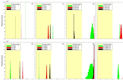
Figure 5 plots the CUE posterior marginal density of the three soil respiration models obtained using the eight data models. The physical range between zero and 0.6 is marked in yellow. Figure 5 shows that the CUE posterior parameter distribution of model 6C (obtained using the data models) that does not account for autocorrelation is within the physi-cally reasonable range. For models 4C and 5C, the posterior parameter samples are outside the range for six data models. For model 4C, the posterior parameters are only within the physical range for the SEP and WSEP data models; for model 5C, the two data models are WLS and WSEP. It is not sur-prising to find the posterior parameter distribution of models 4C and 5C, which have a certain degree of model structure error, to be outside of the physically plausible range. This can be attributed to two reasons. First, the model solution can be biased toward the missing processes in the model structure such as the additional carbon pool in both 4C and 5C or miss-ing the explicit accountmiss-ing for soil moisture in 4C. Second, biased parameter estimation can compensate for model struc-ture inadequacy and other sources of discrepancy in both the physical models and the data models.
In addition, it is important to understand how account-ing for autocorrelation, heteroscedasticity, and non-Gaussian residuals can affect the parameter estimation. First, it is ob-served in Fig. 5e–h that biased parameter estimates are out-side of the physically reasonable range when autocorrelation is explicitly accounted for. This may suggest again that ac-counting for heteroscedasticity is desirable but acac-counting for autocorrelation is not. A possible reason is that filtering autocorrelation may reduce the residual space such that the transformed residual space cannot correspond to the param-eter space of the models. In other words, paramparam-eter informa-tion may be lost due to filtering out autocorrelainforma-tion. However, it is not fully understood why this does not occur for model
6C under data model SLS-AC (Fig. 5e), and more research is warranted. Second, unlike accounting for autocorrelation, ac-counting for heteroscedasticity alone (i.e., WLS and WSEP) only amplifies or reduces the variance without affecting the structure of the residual space. Figure 5c and d show that ac-counting for heteroscedasticity (i.e., WLS and WSEP) tends to improve the parameter estimation in comparison with the homoscedastic data models (i.e., SLS and SEP) shown in Fig. 5a and b. Finally, with respect to non-Gaussian resid-uals, Schoups and Vrugt (2010) suggested that, compared to Gaussian PDF, the peaked PDF of the SEP with a longer tail is useful for making the parameter inference robust against outliers. To a certain degree, this can be substantiated by the results in Fig. 5a–d, in that SEP and WSEP provide more favorable parameter estimates than SLS and WLS.
Finally, Fig. 5a shows that the posterior parameter distri-butions of SLS are very narrow for the three soil respiration models. The narrow distributions can be attributed to several reasons. As a SEP distribution can have longer tails than a Gaussian distribution, this can further increase the sample’s acceptance ratio from tails resulting in a wider distribution (Fig. 5b). In addition, accounting for heteroscedasticity will result in a wider posterior parameter distribution (Fig. 5c) due to accepting higher variances at peak effluxes. More-over, filtering correlation (Fig. 5e–h) increases the entropy, and leads to wider distributions.
4 Results of predictive performance
Based on the last one-third of the CO2efflux observations, a cross-validation test was conducted for the combinations of three soil respiration models and eight data models. For the cross-validation period, the predictive performance is exam-ined using the four statistical metrics defexam-ined in Sect. 2.5. The metrics are also calculated for the calibration period. This is not to perform Bayesian model selection given the calibra-tion data, but to better understand the impact of data models on predictive performance of the three soil respiration mod-els. For each calibration and each cross-validation dataset, a prediction ensemble is generated from the two perspectives: parametric uncertainty only, and total uncertainty. These two perspectives are presented in Sect. 4.1 and 4.2, respectively. 4.1 Predictive performance with parametric
uncertainty of soil respiration model
Figure 5.Marginal posterior parameter density of carbon use efficiency (CUE) for the three soil respiration models and eight data models. The yellow shaded areas represent the reasonable physical range of CUE (0–0.6).
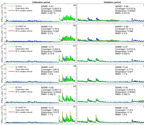
Elshall, 2013). The four statistics above (i.e., NSME, sharp-ness, coverage, and RMS) are calculated for the three soil respiration models and the eight data models. Taking the SLS and WSEP-AC data models as examples, Fig. 6 plots the data (for the calibration and cross-validation periods separately) along with the mean and 95 % credible intervals of the pre-diction ensemble for the three models.
Figure 6 shows that the data models affect model simu-lations for all of the models. The statistics, especially the RMS, indicate that WSEP-AC has better predictive perfor-mance than SLS. This is most visually obvious for model 6C during the cross-validation period after 330 d, as the pre-diction ensemble of SLS (Fig. 6k) cannot cover the obser-vations, whereas the prediction ensemble of WSEP-AC can (Fig. 6l). This conclusion that WSEP-AC outperforms SLS agrees with the conclusion drawn from Figs. 3 and 4.
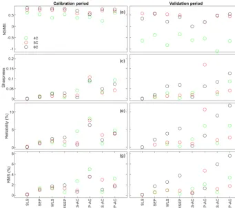
Figure 7 plots the four statistics for all of the soil res-piration models and data models. Figure 7a and b show the predictive performance with respect to the central mean tendency measured by the NSME for both the calibration and cross-validation periods, respectively. The results indi-cate that, under all data models, the low-fidelity model 4C over-fits the data and results in biased predictions, in that the NSME values become significantly worse (e.g., from 0.6 to−0.6) from the calibration to the cross-validation period. This is confirmed by the visual inspection of Fig. 6a and g for
data model SLS and of Fig. 6b and h for data model WSEP-AC. For models 5C and 6C, the NSME values vary with the data models; the central mean accuracy is the worst for SLS-AC that only considers autocorrelation (Fig. 6b).
With respect to the parametric uncertainty estimation, Fig. 7c and d show that sharpness generally increases when the three assumptions in the data models are gradually re-laxed from SLS to WSEP-AC. This is even more obvious during the validation period. Given that the prediction en-semble does not center on the data, the increasing sharpness is desirable as it improves reliability. This is confirmed by the reliability plots in Fig. 7e and f. The exceptions are once again for SLS-AC and SEP-AC that generally have the low-est coverage.
With respect to the overall predictive performance mea-sured by the RMS, the same variation pattern and exception are also observed in the RMS plots in Fig. 7g and h. This is not surprising because the RMS is the metric that can be used to measure all three criteria (central mean tendency, sharp-ness, and reliability). As the prediction ensemble is not cen-tered on the data, the sharpness and reliability are the decisive factors for evaluating the predictive performance.
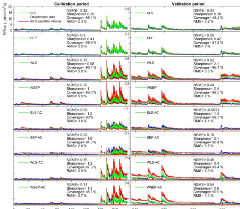
Figure 6.Observation data (blue dots), mean prediction (green line), and 95 % credible intervals (red line) of prediction ensembles for (a–f)the calibration period and(g–l)the validation period. The plots are for the three soil respiration models using the SLS and WSEP-AC data models. The prediction ensembles are generated to consider parametric uncertainty of the soil respiration models only. The model prediction accuracy, reliability, dispersion and overall predictive performance are measured by the Nash–Sutcliffe model efficiency (NSME), the predictive coverage metric (“Coverage”), the sharpness metric (“Sharpness”) and the relative model score (RMS), respectively.
residuals using the Gaussian and SEP distributions, the con-clusion is that the SEP distribution outperforms the Gaussian distribution with respect to predictive performance. Finally, uncertainty underestimation is evidenced by the very small predictive coverage. The underestimation of uncertainty for all of the physical models with all of the data model is not un-expected because only parametric uncertainty is considered in this study. Considering the overall predictive uncertainty is the subject of the next section.
4.2 Predictive performance with total uncertainty
The simulated output Y(θp) is generally not equal to the observed output d, and we have a residual term ε due to measurement, input, and model structure errors such that
Figure 7. (a, b)Nash–Sutcliffe model efficiency (NSME),(c, d)sharpness,(e, f)predictive coverage, and(g, h)relative model score for measuring predictive performance of the three soil respiration models and the eight data models during the calibration and cross-validation periods. The statistics are evaluated from the prediction ensembles generated to consider parametric uncertainty of the soil respiration models only.
the residual error includes errors in measurements, model in-puts, and model structures (e.g., Thyer et al., 2009; Schoups and Vrugt, 2010). This lumped approach is based on sam-pling the residuals modelε(θε)with parametersθε. SLS has one fixed parameter, the constant variance, and other data models have two to six parameters. Thus, in this section the prediction ensemble addresses parametric uncertainty of not only the soil respiration models but also the data mod-els. When generating the prediction ensemble in the proce-dure described by Schoups and Vrugt (2010), an ensemble of residuals is first generated by running the data models with posterior samples of the data model parameters for the positive carbon efflux domain; the residual ensemble is then added to the prediction ensemble generated in Sect. 4.1.
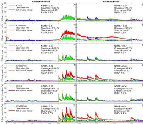
We start by undertaking a visual assessment of the predic-tive performance. Figure 8 is similar to Fig. 6 with the excep-tion that Fig. 8 considers the overall predictive uncertainty (i.e., parametric and output uncertainty), whereas Fig. 6 only considers the parametric uncertainty. Figure 8 reveals a prac-tical observation about accounting for the overall uncertainty using the lumped approach of sampling the data models. For example, Fig. 8b shows that, despite the wide prediction in-terval of model 4C, the model with significant model
struc-ture error cannot capstruc-ture the birch pulse around day 180. It indicates that properly using a data model for model residu-als cannot compensate for significant model structure error.
Figure 9 plots the four statistics (NSME, sharpness, pre-dictive coverage, and RMS) of the three soil respiration mod-els under the eight data modmod-els to assess the predictive per-formance. With respect to the central mean tendency, the NSME values in Fig. 9a and b are visually the same as those in Fig. 7a and b, indicating that the central mean accuracy under parametric uncertainty is the same as that under pre-dictive uncertainty.
Figure 8.Observation data (blue dots), mean prediction (green line), and 95 % credible intervals (red line) of prediction ensembles for(a– f)the calibration period and(g–l)the validation period. The plots are for the three soil respiration models using the SLS and WSEP-AC data models. The prediction ensembles are generated to consider parametric uncertainty of not only the soil respiration models but also the data models. The model prediction accuracy, reliability, dispersion and overall predictive performance are measured by the Nash–Sutcliffe model efficiency (NSME), the predictive coverage metric (“Coverage”), the sharpness metric (“Sharpness”) and the relative model score (RMS), respectively.
With respect to the overall predictive performance, the RMS values are largely determined by the mean accuracy and sharpness as the predictive coverage is similar for differ-ent data models. Figure 9g and h of RMS show that the pre-dictive performance of the four data models that account for autocorrelation is worse than that of the other four data mod-els. This suggests again that one needs to be cautious when building autocorrelation into a data model. This is consistent with the finding of Evin et al. (2013, 2014) that accounting for autocorrelation before accounting for heteroscedasticity or jointly accounting for autocorrelation and heteroscedas-ticity can result in poor predictive performance. In summary,
Figure 9. (a, b)Nash–Sutcliffe model efficiency (NSME),(c, d)sharpness,(e, f)predictive coverage, and(g, h)relative model score for measuring predictive performance of the three soil respiration models and the eight data models during the calibration and cross-validation periods. The statistics are evaluated from the prediction ensembles generated to consider parametric uncertainty of not only the soil respiration models but also the data models.
To demonstrate the impacts of the data models on the predictive performance of the soil respiration models, Fig. 10 plots the model simulations and predictions given by model 6C during the calibration and cross-validation pe-riods using all the eight data models. Figure 10 is used to investigate predictive performance characteristics of the dif-ferent data models. By examining the predictive performance of model 6C, specific predictive performance patterns can be identified. Figure 10a–d show that SLS and SEP have similar predictive performance with SEP generally having better pre-dictive performance especially during the validation period. Not accounting for heteroscedasticity will underestimate the predication uncertainty (Fig. 10b, d). This is mainly because the variance of the efflux residuals increases with the magni-tude of the carbon effluxes (Fig. 3a); thus, assuming constant variance is not representative. Accordingly, accounting for heteroscedasticity using WLS (Fig. 10e) or WSEP (Fig. 10h) will make the predictions more sensitive to peak carbon ef-fluxes. This will generally improve the predictive coverage on the expense of sharpness and the central mean tendency. While WLS and WSEP have similar predictive performance, WSEP has better central mean tendency and overall predic-tive performance than WLS. Figure 10i–l show that
account-ing for autocorrelation usaccount-ing SLS-AC and SEP-AC results in wider uncertainty bands and insensitivity to peak carbon effluxes compared with SLS and SEP (Fig. 10a–d), which may be due to the reduction in the information content of the residuals. This results in the deterioration of the sharpness, the central mean tendency, and the capturing of peak carbon fluxes, especially during the validation period. Figure 10m–p show that accounting for both heteroscedasticity and autocor-relation using WLS-AC and WSEP-AC makes the inference robust against peak carbon effluxes. However, due to the loss of information content, the uncertainty bands are still wider, and the uncertainty becomes overestimated especially during validation period compared with WLS and WSEP (Fig. 10e– h). The results of models 4C and 5C, which are not shown here, also display the same prediction patterns with respect to non-Gaussian residuals, heteroscedasticity, and autocorre-lation.
co-Figure 10.Observation data (blue dots), mean prediction (green line), and 95 % credible intervals (red line) for 6C for the eight likelihood functions during the calibration period(a–h)and the validation period(i–p). The prediction ensembles are generated to consider parametric uncertainty of not only the soil respiration models but also the data models. The model prediction accuracy, reliability, dispersion and overall predictive performance are measured by the Nash–Sutcliffe model efficiency (NSME), the predictive coverage metric (“Coverage”), the sharpness metric (“Sharpness”) and the relative model score (RMS), respectively. For clarity, theyaxis markers and label are only displayed for the first subplot and are the same for all subplots.
efficient of 0.92. However, we note that for models 4C and 5C the overall predictive performances during the calibration and validation periods are not as well correlated as for 6C, with correlation coefficients of 0.52 for model 4C and 0.61 for model 5C. This suggests that model 6C is more robust than 4C and 5C for forecasting and hindcasting.
4.3 Discussion on handling residual correlation
Accounting for autocorrelation can lead to biased param-eter estimation (Fig. 5) and poor predictive performance (Fig. 10). Autocorrelated residuals may be attributed to
model discrepancy, as shown in Lu et al. (2013). The most obvious solution to handle the autocorrelation is to reduce the autocorrelation by improving the soil respiration model. If model improvement is difficult for practical reasons, we can improve the data model to better characterize the au-tocorrelation. Addressing autocorrelation in a data model is challenging, as it involves several interlinked factors as fol-lows:
uals based on the covariance matrix of residualsL(e)
(e.g., Lu et al., 2013), or to normalized residualsL(a)
(e.g., Schoups and Vrugt, 2010; Evin et al., 2013). Note that “e” is a vector of transformed residuals, whereas “a” denotes a vector of independent and identically dis-tributed random errors with a zero mean and unit stan-dard deviation. TheL(e)approach based on covariance matrix of residuals is generally limited to Gaussian data models (e.g., Lu et al., 2013), whereas the L(a) ap-proach for normalized residuals can be readily adopted for non-Gaussian data models.
3. The autocorrelation model could have an impact. Us-ing an autoregressive model is a popular technique to account for autocorrelated residuals. However, using an autoregressive model with either a joint inversion ap-proach (e.g., this study and Schoups and Vrugt, 2010) or sequential approaches (e.g., Evin et al., 2013, 2014; Lu et al., 2013) removes correlation errors via a filter approach, which can lead to a loss of information con-tent. As this may cause an overcorrection of prediction especially at surge events, Li et al. (2015) developed a restricted autoregressive model to overcome this ad-verse effect. Other autocorrelation models include the moving average model and the mixed autoregressive-moving averaging model (Chatfield, 2003).
4. Joint vs. sequential inversion for autocorrelation could have an impact. Sequential inversion approaches in-clude two-step procedures (e.g., Evin et al., 2013, 2014; Lu et al., 2013) or the multi-step procedure (M. Li et al., 2016). These sequential approaches estimate the au-toregressive parameters sequentially in a later step af-ter estimating the physical model parameaf-ters and other data model parameters. Evin et al. (2013, 2014) used a sequential approach to avoid the interaction between the parameters of the heteroscedasticity model and the autocorrelation model. In addition, the autoregressive model parameters can be deterministically calculated as internal variables of the data model similar to Lu et al. (2013), and not as calibration parameters (e.g., Schoups and Vrugt, 2010; Evin et al., 2013, 2014). While the first step in the sequential approach would avoid the biased parameter estimation (Fig. 10a–d), the second step can still lead a poor predicative perfor-mance as we are essentially using a filter approach to remove residual correlation. To address this problem, M. Li et al. (2016) utilizes a multi-step procedure that is
5 Conclusions
In parameter estimation and prediction of soil carbon fluxes to the atmosphere, one often assumes that residuals, which include errors in observations, model inputs, parameter es-timates, and model structures, are normally distributed, ho-moscedastic, and uncorrelated. We study these assumptions by calibrating three soil respiration models, which have vary-ing degrees of model structure errors. We further explore eight data models that statistically characterize the residuals; we start with the standard least squares (SLS) and skew expo-nential power (SEP) data models that assume homoscedastic and non-correlated residuals. For these two distributions, we evaluate six other data models that account for heteroscedas-ticity (WLS and WSEP), autocorrelation (SLS-AC and SEP-AC), and joint inversion of heteroscedasticity and autocor-relation (WLS-AC and WSEP-AC). To our knowledge this is the first study that provides such a detailed analysis for soil reparation inverse modeling. We also use three soil res-piration models with different degrees of model fidelity (i.e., model discrepancy) and model complexity (i.e., number of model parameters) to understand the impact of model dis-crepancy on the calibration results under different data mod-els. We analyze the results with respect to (1) residual char-acterization, (2) parameter estimation, (3) predictive perfor-mance, and (4) impacts of model discrepancy. The main find-ings of this study are summarized as follows:
1. With respect to residual characterization, residual anal-ysis results suggest that the common assumption of not accounting for heteroscedasticity and residual autocor-relation in the SLS and SEP data models results in the poor characterization of residuals. Explicitly accounting for heteroscedasticity in WLS and WSEP results in the significantly improved characterization of the residuals, and the improvement is larger than that obtained by ac-counting for both heteroscedasticity and autocorrelation in WSL-AC and WSEP-AC. Accounting for autocorre-lation only in SLS-AC and SEP-AC does not signifi-cantly improve the characterization of the residuals. 2. With respect to parameter estimation, the impacts of the
au-tocorrelation tend to yield CUE estimates that are phys-ically unreasonable. We speculate that filtering residual correlation can affect the mapping of the model physics (as implicitly included in the residuals) into the param-eter space, which might result in biased paramparam-eter esti-mates that are physically unreasonable.
3. With respect to predictive performance, it is measured by four statistical criteria: central mean tendency, sharp-ness, coverage, and relative model score for both the calibration and the cross-validation periods. Results show that accounting for autocorrelation in SLS-AC, SEP-AC, WLS-AC, and WSEP-AC reduces the predica-tive performance, such that the predicpredica-tive performance is inferior to that of SLS in terms of the central mean tendency and overall predictive performance (measured by the relative model score), especially during the cross-validation period. Results also indicate that using the SEP distribution can potentially improve the predictive performance. The same is true for accounting for het-eroscedasticity. Using the SEP distribution and account-ing for heteroscedasticity (i.e., WSEP) can potentially improve the predictive performance.
4. With respect to the impact of model discrepancy, the high-fidelity model (6C) gives the best results with re-spect to parameter estimation and predictive perfor-mance. Model 6C generally maintains its superior per-formance under different data models. This justifies the complexity of model 6C relative to model 5C that has one less carbon pool. Model 4C, with the lowest fidelity, maintains its poor performance for different data mod-els, because the model only has four carbon pools and lacks the explicit representation of soil moisture control. Based on the empirical findings above, we conclude the following:
1. Not accounting for heteroscedasticity and autocorrela-tion using a Gaussian or non-Gaussian data model might not necessarily result in biased parameter estimates or biased predictions with respect to the central mean ten-dency, but will definitely underestimate uncertainty re-sulting in lower overall predictive performance. 2. Using a non-Gaussian data model can improve the
pa-rameter estimation and predictive performance with re-spect to the central mean tendency and the uncertainty quantification.
3. Accounting for heteroscedasticity improves the uncer-tainty estimation with respect to reliability at the cost of having a wider predictive interval.
4. This study confirms other empirical findings and theo-retical analyses (Evin et al., 2013, 2014; Li et al., 2015; Ammann et al., 2018) which propose that separately ac-counting for autocorrelation or jointly acac-counting for
autocorrelation and heteroscedasticity can be problem-atic. While the reasons remain poorly understood (Am-mann et al., 2018), this might be attributed to non-stationarity due to wet–dry periods with half-hourly data (Ammann et al., 2018) or to the method of handling autocorrelation (e.g., Schoups and Vrugt, 2010; Evin et al., 2013, 2014; Lu et al., 2013; M. Li et al., 2015, 2016; Ammann et al., 2018). Further investigation to address autocorrelation in soil respiration modeling is warranted in a future study.
The above conclusions are subject to several limitations. First, the conclusions are specific to the soil respiration mod-els developed and validated for semi-arid savannah land-scapes. Performance variations across different soil respira-tion models with different levels of complexity are possible. Second, the conclusions are conditioned on data that were obtained at half-hourly intervals over a 1-year period. Differ-ent conclusions would be possible if the data were thinned to daily or weekly scales or data from longer observation peri-ods were used. Third, our study investigates the effects of the residual assumptions of formal likelihood functions via di-rect conditioning of the residuals model parameters, yet this can also be undertaken using other approaches such as resid-uals transformation (Thiemann et al., 2001), autoregressive bias models (Del Giudice et al., 2013), approximate Bayesian computation (Sadegh and Vrugt, 2013), and data assimila-tion (Spaaks and Bouten, 2013). Comparing different meth-ods for accounting for the residual assumptions are beyond the scope of this work. Fourth, this study focuses on formal Bayesian computation using formal likelihood functions, and comparison with other inference functions such as informal likelihood functions or approximate Bayesian computation is warranted in a future study.
Based on the aforementioned conclusions and limitations, we recommend beginning the calibration of soil respira-tion models with simple SLS or SEP likelihood funcrespira-tion. If the residuals characterization is adequate (e.g., Scharnagl et al., 2011), then the underlying assumptions are met. Other-wise, the complexity of the data model can be increased until satisfactory results are obtained in terms of residuals char-acterization, posterior parameter estimation, and predictive performance. This is similar to the procedure given in Smith et al. (2015). Although the empirical findings of this study provide general guidelines for data model selection for soil respiration modeling, more comparative studies are needed to validate or refute the findings of this study.
MCMC Markov chain Monte Carlo MIC Microbial biomass
NSME Nash–Sutcliffe model efficiency PDF Probability density function RMS Relative model score
SEP Skew exponential power distribution
SEP-AC Skew exponential power distribution with autocorrelation SLS Standard least square
SLS-AC Standard least square with autocorrelation SOC Soil organic carbon
WLS Weighted least squared
WLS-AC Weighted least squared with autocorrelation WSEP Weighted skew exponential power distribution
Supplement. The supplement related to this article is available online at: https://doi.org/10.5194/gmd-12-2009-2019-supplement.
Author contributions. ASE developed and implemented the code for the eight data models for soil respiration modeling, and prepared the paper with contributions from all co-authors. MY developed the research idea and outline, and supervised the research implementa-tion while ASE was a post-doc at Florida State University. GN de-veloped the soil respiration models. GAB collected and processed the eddy-covariance data used for model calibration.
Competing interests. The authors declare that they have no conflict of interest.
Acknowledgements. The first two authors were supported by the U.S. Department of Energy grant no. DE-SC0008272. The first au-thor was also partly supported by the U.S. National Science Foun-dation award no. OIA-1557349. The second author was also partly supported by U.S. Department of Energy grant no. DE-SC0019438 and U.S. National Science Foundation grant no. EAR-1552329. We thank the two anonymous reviewers for providing comments that helped to improve the paper.
Review statement. This paper was edited by Christoph Müller and reviewed by two anonymous referees.
References
Ahrens, B., Reichstein, M., Borken, W., Muhr, J., Trumbore, S. E., and Wutzler, T.: Bayesian calibration of a soil organic carbon model using114C measurements of soil organic carbon and het-erotrophic respiration as joint constraints, Biogeosciences, 11, 2147–2168, https://doi.org/10.5194/bg-11-2147-2014, 2014. Allison, S. D., Wallenstein, M. D., and Bradford, M. A.: Soil-carbon
response to warming dependent on microbial physiology, Nat. Geosci., 3, 336–340, https://doi.org/10.1038/ngeo846, 2010. Ammann, L., Reichert, P., and Fenicia, F.: A framework for
like-lihood functions of deterministic hydrological models, Hydrol. Earth Syst. Sci. Discuss., https://doi.org/10.5194/hess-2018-406, in review, 2018.
Bagnara, M., Sottocornola, M., Cescatti, A., Minerbi, S., Mon-tagnani, L., Gianelle, D., and Magnani, F.: Bayesian op-timization of a light use efficiency model for the es-timation of daily gross primary productivity in a range of Italian forest ecosystems, Ecol. Model., 306, 57–66, https://doi.org/10.1016/j.ecolmodel.2014.09.021, 2015. Bagnara, M., Oijen, M. Van, Cameron, D., Gianelle, D.,
Magnani, F., and Sottocornola, M.: Bayesian calibration of simple forest models with multiplicative mathematical structure: A case study with two Light Use Efficiency models in an alpine forest, Ecol. Model., 371, 90–100, https://doi.org/10.1016/j.ecolmodel.2018.01.014, 2018.
Barr, J. G., Engel, V., Fuentes, J. D., Fuller, D. O., and Kwon, H.: Modeling light use efficiency in a subtropical mangrove forest equipped with CO2eddy covariance, Biogeosciences, 10, 2145– 2158, https://doi.org/10.5194/bg-10-2145-2013, 2013.
Barron-Gafford, G. A., Scott, R. L., Jenerette, G. D., and Hux-man, T. E.: The relative controls of temperature, soil mois-ture, and plant functional group on soil CO2 efflux at diel, seasonal, and annual scales, J. Geophys. Res., 116, G01023, https://doi.org/10.1029/2010JG001442, 2011.
Barron-Gafford, G. A., Cable, J. M., Bentley, L. P., Scott, R. L., Huxman, T. E., Jenerette, G. D., and Ogle, K.: Quanti-fying the timescales over which exogenous and endogenous conditions affect soil respiration, New Phytol., 202, 442–454, https://doi.org/10.1111/nph.12675, 2014.
Berryman, E. M., Frank, J. M., Massman, W. J., and Ryan, M. G.: Agricultural and Forest Meteorology Using a Bayesian framework to account for advection in seven years of snowpack CO2 fluxes in a mortality-impacted subalpine forest, Agr. Forest Meteorol., 249, 420–433, https://doi.org/10.1016/j.agrformet.2017.11.004, 2018.
Box, G. E. P. and Tiao, G. C.: Bayesian inference in statistical anal-ysis, Wiley, New York, 1992.
Braakhekke, M. C., Beer, C., Schrumpf, M., Ekici, A., Ahrens, B., Hoosbeek, M. R., Kruijt, B., Kabat, P., and Reich-stein, M.: The use of radiocarbon to constrain current and future soil organic matter turnover and transport in a temperate forest, J. Geophys. Res.-Biogeo.,119, 372–391, https://doi.org/10.1002/2013JG002420, 2014.
Bradford, M. A., Davies, C. A., Frey, S. D., Maddox, T. R., Melillo, J. M., Mohan, J. E., Reynolds, J. F., Treseder, K. K., and Wallenstein, M. D.: Thermal adaptation of soil microbial respiration to elevated temperature, Ecol. Lett., 11, 1316–1327, https://doi.org/10.1111/j.1461-0248.2008.01251.x, 2008. Braswell, B. H., Sacks, W. J., Linder, E., and Schimel, D. S.:
Estimating diurnal to annual ecosystem parameters by synthe-sis of a carbon flux model with eddy covariance net ecosys-tem exchange observations, Glob. Change Biol., 11, 335–355, https://doi.org/10.1111/j.1365-2486.2005.00897.x, 2015. Cable, J. M., Ogle, K., Williams, D. G., Weltzin, J. F., and
Huxman, T. E.: Soil Texture Drives Responses of Soil Res-piration to Precipitation Pulses in the Sonoran Desert: Im-plications for Climate Change, Ecosystems, 11, 961–979, https://doi.org/10.1007/s10021-008-9172-x, 2008.
Cable, J. M., Ogle, K., Lucas, R. W., Huxman, T. E., Loik, M. E., Smith, S. D., Tissue, D. T., Ewers, B. E., Pendall, E., Welker, J. M., Charlet, T. N., Cleary, M., Griffith, A., Nowak, R. S., Rogers, M., Steltzer, H., Sullivan, P. F., and Van Ges-tel, N. C.: The temperature responses of soil respiration in deserts: a seven desert synthesis, Biogeochemistry, 103, 71–90, https://doi.org/10.1007/s10533-010-9448-z, 2011.
Chatfield, C.: The analysis of time series: an introduction, Chapman & Hall/CRC, Boca Raton, 2003.