https://doi.org/10.5194/gmd-12-1791-2019 © Author(s) 2019. This work is distributed under the Creative Commons Attribution 4.0 License.
Efficient surrogate modeling methods for large-scale Earth system
models based on machine-learning techniques
Dan Lu1and Daniel Ricciuto2
1Computational Sciences and Engineering Division, Climate Change Science Institute, Oak Ridge National Laboratory, Oak Ridge, TN, USA
2Environmental Sciences Division, Climate Change Science Institute, Oak Ridge National Laboratory, Oak Ridge, TN, USA
Correspondence:Dan Lu ([email protected])
Received: 18 December 2018 – Discussion started: 17 January 2019
Revised: 22 March 2019 – Accepted: 17 April 2019 – Published: 6 May 2019
Abstract.Improving predictive understanding of Earth sys-tem variability and change requires data–model integration. Efficient data–model integration for complex models re-quires surrogate modeling to reduce model evaluation time. However, building a surrogate of a large-scale Earth system model (ESM) with many output variables is computation-ally intensive because it involves a large number of expen-sive ESM simulations. In this effort, we propose an efficient surrogate method capable of using a few ESM runs to build an accurate and fast-to-evaluate surrogate system of model outputs over large spatial and temporal domains. We first use singular value decomposition to reduce the output di-mensions and then use Bayesian optimization techniques to generate an accurate neural network surrogate model based on limited ESM simulation samples. Our machine-learning-based surrogate methods can build and evaluate a large sur-rogate system of many variables quickly. Thus, whenever the quantities of interest change, such as a different objec-tive function, a new site, and a longer simulation time, we can simply extract the information of interest from the surro-gate system without rebuilding new surrosurro-gates, which signif-icantly reduces computational efforts. We apply the proposed method to a regional ecosystem model to approximate the relationship between eight model parameters and 42 660 car-bon flux outputs. Results indicate that using only 20 model simulations, we can build an accurate surrogate system of the 42 660 variables, wherein the consistency between the surro-gate prediction and actual model simulation is 0.93 and the mean squared error is 0.02. This highly accurate and fast-to-evaluate surrogate system will greatly enhance the
computa-tional efficiency of data–model integration to improve pre-dictions and advance our understanding of the Earth system.
1 Introduction
use very few simulation model runs to build an accurate and quickly evaluated surrogate system of a large-scale problem based on advanced machine-learning methods.
In Earth system modeling, we usually need to build a sur-rogate system of many output variables over large spatial and temporal domains. ESMs tend to be simulated on a regional or global scale with many grid cells for several years, pro-ducing a large number of output variables. In addition, ESMs are used to solve versatile scientific problems, so the quan-tities of interest (QoIs) often change. Moreover, the devel-opment of a surrogate requires expensive ESM runs, and a large number of runs are often needed to capture the complex model input–output relationship. Therefore, it is reasonable to build a surrogate system for all possible model outputs to reduce the efforts of rerunning ESMs for a new surrogate de-velopment when the QoIs change. In this way, whenever we simulate the outputs in a new site or for additional sites at a different time or for a longer period, we can simply extract the information of interest from the large surrogate system without spending extra efforts to build new surrogates, which significantly reduces computational costs.
Building and evaluating a surrogate system of a large num-ber of model outputs can be very computationally intensive for almost all the surrogate methods. Polynomials and artifi-cial neural networks are widely used for surrogate modeling (Razavi et al., 2012; Viana et al., 2014). Polynomial meth-ods, such as polynomial regression and radial basis functions, need to solve polynomial coefficients in the surrogate con-struction and to calculate matrix multiplications in the sur-rogate evaluation. Using apth-order polynomial to approx-imate a model withd parameters,M=(p+d)!/(p!d!) co-efficients need to be solved; i.e., the number of coco-efficients increases factorially fast with the parameter size and poly-nomial order. Whend=40, a second-order polynomial in-volves 861 coefficients and a third-order polynomial inin-volves 12 341 coefficients. ESMs have many uncertain parameters, and a high-order polynomial is usually needed to approxi-mate complex ESMs, which can easily lead to a prohibitive number of model evaluations, up to∼105, necessary to com-pute the polynomial coefficients. To reduce the computa-tional costs, some regularization techniques such as Bayesian compressive sensing have been used (Sargsyan et al., 2014; Ricciuto et al., 2018). These regularization techniques can use a few samples to solve a large number of coefficients (i.e., an underdetermined system) by iteratively minimizing the L1 norm of the coefficient vector. But they usually perform min-imization once for one model output, so for a large model output problem, significant computing effort is required. To reduce the computing burden in building polynomial-based surrogates, we need to reduce the output dimensions.
Reducing the model output dimensions also improves computational efficiency in the evaluation of the polynomial-based surrogates. For example, evaluating the third-order polynomial-based surrogate of the model with 40 parameters and 300 000 outputs for one parameter sample, we need to
calculate two matrix multiplications for which matrixAhas the size [1,M],Bhas the size [M,Nout],M=12 341, and
Nout=300 000. The surrogate evaluation takes about 90 s and most time is spent on loading the huge matrix. When
Nout is reduced to 20, the surrogate evaluation is quickly reduced to less than a second. Note that an ESM can eas-ily have more than 40 parameters and more than 300 000 model outputs. Even using the most advanced supercomput-ers with GPUs, the data storage and loading are still a bottle-neck. Thus, reducing model output dimensions is necessary for quickly building and evaluating polynomial-based surro-gates.
Surrogate modeling assisted by a neural network (NN) also suffers from high computational costs when applied to a large-scale problem with many QoIs. To approximate a com-plex ESM with many outputs, a complicated NN with many wide hidden layers is usually needed to capture the complex relationship between the model inputs and outputs because each spatial and temporal output variable is driven by differ-ent meteorological forcing such as air temperature, humid-ity, wind speed, precipitation, and radiation. The full con-nections between nodes in the input layer and the first hid-den layer, between nodes of the hidhid-den layers, and between nodes in the last hidden layer and a large number of nodes on the output layer involve a large number of NN weights and biases that need to be solved. For the same example dis-cussed above, to approximate the model with 40 parameters and 300 000 model outputs, an NN with two hidden layers and each layer having 100 nodes has over 30 million weights and biases. Calculation of these weights and biases requires many samples to train the NN for a good fit. Each training sample involves one model evaluation. However, ESM sim-ulation is time consuming, which usually takes several hours or days and can be up to months or even years. A limited sample size is not enough to train a deep and wide NN for convergence, and a simple NN trained by a small sample size may not capture underlying Earth systems accurately. Thus, reducing model output dimensions is needed to advance NN-based surrogate modeling. A small output size reduces the width of the output layer and also simplifies the relationship between the model inputs and outputs so that a simple NN architecture can be appropriate and a small sample size can be sufficient to accurately train the simple NN. In addition, a simple NN can also be evaluated fast with small weight matrix multiplications.
meth-ods, NNs have shown less difficulty in fitting highly nonlin-ear and discontinuous functions that are usually observed in ESM response surfaces. For example, carbon flux state vari-ables, such as gross primary productivity (GPP), are strongly affected by vegetation-related parameters. When the parame-ter samples cause zero vegetation growth, GPP has zero val-ues, whereas when the parameter samples cause high vege-tation growth, GPP has large positive values. This leads to a discontinuous GPP response surface jumping from zeros to nonzeros.
NNs can theoretically fit any functions, but their prac-tical performance strongly depends on the NN’s architec-tures and hyperparameters. An NN has many hyperparam-eters such as the number of layers, number of nodes in each layer, type of activation functions, and learning rate of the stochastic gradient descent optimization. A slight change in the hyperparameter value can result in dramatically different NN performance. Development of a high-performing NN is time-intensive and usually requires trial-and-error tuning by machine-learning experts. In this work, we use Bayesian op-timization techniques to optimize the NN architecture and hyperparameters to produce an accurate NN model for the training data. Bayesian optimization searches the hyperpa-rameter space to iteratively minimize the validation errors of the NN by balancing exploration and exploitation (Shahriari et al., 2016). Research has suggested that Bayesian hyperpa-rameter optimization of NNs is more efficient than manual, random, or grid search with better overall performance on test data and less time required for optimization (Bergstra et al., 2011; Snoek et al., 2012). Bayesian optimization in-volves a large ensemble of NN fittings, and it is a sequential model-based optimization; thus, fast training of the NN mod-els is important. Our proposed SVD method can simplify the NN architecture to advance the NN training and improve the Bayesian optimization performance.
In this effort, we propose an SVD-enhanced, Bayesian-optimized, and NN-based surrogate method and aim to build an accurate and fast-to-evaluate surrogate system of a large-scale model using few model runs to improve computa-tional efficiency in surrogate modeling and thus advance the data–model integration. We apply the method to a simpli-fied land model in the Energy Exascale Earth System Model (sELM) to improve the model predictive capability of car-bon fluxes. We build a surrogate system of 42 660 model output variables, which are annual GPPs at 1422 locations simulated for 30 years. The sELM is a regional-scale ter-restrial ecosystem model that simulates terter-restrial water, en-ergy, and biogeochemical processes in terrestrial surfaces. Simulation of sELM is important for improving our under-standing of ecosystem responses to climate change. How-ever, sELM requires lengthy times for hydrologic and carbon cycle equilibration, and these high computational costs limit the affordable number of simulations in data–model integra-tion, thus resulting in poor model performance. The proposed machine-learning-assisted surrogate method makes
sophis-ticated data–model integration computationally feasible and promises an improvement of the sELM predictions.
The major contributions of this work are the following: (1) using SVD to reduce model output dimensions to im-prove computational efficiency in both building and evalu-ating an accurate surrogate of a large-scale ESM; (2) using Bayesian optimization techniques to quickly generate an ac-curate NN-based surrogate; and (3) applying the proposed method to build a large surrogate system of a regional-scale ESM to advance data–model integration. To our knowledge, the method of using SVD to enhance surrogate modeling is novel and we have not seen the application of Bayesian op-timization to improve NN-based surrogates in Earth system modeling.
The paper is organized as follows. In Sect. 2, we first de-scribe the sELM, the model parameters, and the QoIs we build surrogates for; following that, we introduce the SVD, NNs, and Bayesian optimization methods. In Sect. 3, we ap-ply the methods to the sELM and analyze the surrogate ac-curacy. In Sect. 4, we discuss strategies to improve surrogate accuracy and investigate our method’s performance in the ap-plication of these strategies. In Sect. 5, we end this paper by drawing our conclusions.
2 Materials and methods
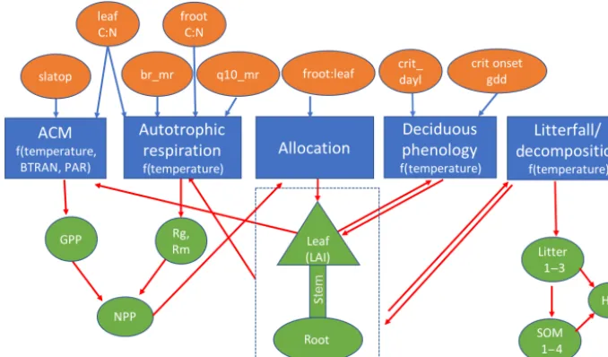
2.1 Description of sELM and related parameters We developed a simplified version of Energy Exascale Earth System (E3SM) land model (ELM), or sELM, to simulate carbon cycle processes relevant for Earth system models in a computationally efficient framework. This framework al-lows us to perform large regional ensembles that are compu-tationally infeasible using offline land surface models such as ELM. The sELM is a combination of model elements from the Data Assimilation Linked Ecosystem Carbon model (DALEC; Williams et al., 2005) and the Community Land Model version 4.5 (CLM4.5; Oleson and Lawrence, 2013). The sELM consists of five process-based submodels that simulate carbon fluxes between five major carbon pools us-ing 49 overall parameters. Based on previous sensitivity anal-ysis using ELM (Ricciuto et al., 2018), this study considers the most sensitive eight parameters associated with four out of the five submodels. We summarize all five process-based submodels and their interactions below and in Fig. 1.
Figure 1.Schematic of sELM, with processes shown using blue boxes with dependencies on environmental data; eight uncertain parameter inputs are listed in orange ovals, and model state variables are indicated by green shapes. Parameters are input to one or more processes as indicated by blue arrows. Model state variables may be outputs for some processes and input for other processes as indicated by red arrows.
which reduces GPP when soil water is insufficient to support transpiration. Because sELM does not predict soil moisture, BTRAN is calculated in a full ELM simulation and is fed into sELM as an input. ACM shares one parameter, the ratio of leaf carbon to nitrogen (leaf C : N), with the autotrophic respiration model and employs an additional parameter, the specific leaf area at the top of the canopy (slatop).
The remaining four submodules are based on ELM. The autotrophic respiration model computes the growth and maintenance respiration components and is controlled by four parameters, the leaf C : N, the ratio of fine root car-bon to nitrogen (froot C : N), the base rate of maintenance respiration (br_mr), and temperature sensitivity for mainte-nance respiration (q10_mr). The allocation model partitions carbon to several vegetation carbon pools following those in ELM: leaves, fine roots, live stem, dead stem, live coarse roots, and dead coarse roots. In the allocation model, we only consider one parameter, the ratio of fine root to leaf allocation (froot_leaf). The deciduous phenology model is used to predict the timing of budbreak and senescence. It considers two parameters, the critical day length to initi-ate autumn senescence (crit_dayl) and the number of accu-mulated growing degree days needed to initiate spring leaf-out (crit_onset_gdd). The last submodel is a decomposition model that simulates heterotrophic respiration and the de-composition of litter into soil organic matter using the con-verging trophic cascade framework as in the CLM4.5 (Ole-son and Lawrence, 2013). Because this study focuses on plant carbon uptake, no uncertain parameters are considered in the decomposition model. In sELM, nutrient feedbacks are not represented explicitly; however, a constant nitrogen
lim-itation factor is included to downregulate photosynthetic up-take.
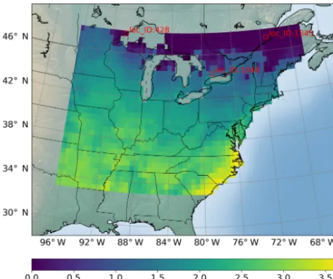
Figure 2. Locations of interest for which we build surrogates of GPP (g C m−2d−1) variables; a total of 1422 locations are consid-ered. The figure shows the sELM-simulated annual GPP based on one parameter sample.
used for developing the surrogate and some of them are used to evaluate the surrogate accuracy, as discussed in Sect. 3. 2.2 Efficient surrogate modeling methods
In this section, we introduce our SVD-enhanced, Bayesian-optimized, and NN-based surrogate methods. We first de-scribe the SVD for reducing data dimensionality, then intro-duce the NN techniques for building a surrogate model, and last depict the Bayesian optimization algorithm for produc-ing a high-performproduc-ing NN-based surrogate.
2.2.1 Singular value decomposition for data compression
We build a surrogate system of model outputs by fitting a data matrix whose columns are output variables and rows are output samples. For a model with 100 000 output variables, the columns of this matrix span a 100 000-dimensional space. Encoding this matrix on a computer takes quite a lot of mem-ory and evaluating this matrix takes a large number of calcu-lations. We are interested in approximating this matrix with some low-rank matrix but retaining most of its information to reduce data transfer and accelerate matrix calculation.
Singular value decomposition (SVD) decomposes a ma-trixAwith sizem×ninto three other matrices:A=USVT, whereUis an m×morthogonal matrix,Vis an n×n or-thogonal matrix, and Sis an m×ndiagonal matrix saving singular values in descending order on the diagonal. Trun-cated SVD keeps the K largest singular values and corre-spondingKcolumn vectors ofUandKrow vectors ofVT to form eA=UK SKVTK. TheK-rank matrixeA has proven
to be the best approximation ofAin minimizing the Frobe-nius norm of the difference betweenAandeAunder the con-straint of rank (eA)=K. In addition, the total of the firstK singular values divided by the sum of all the singular values is the percentage of information that those singular values contain (i.e., the percentage of the total variance explained by those singular values). For example, if we want to keep 90 % of the data information, we just need to compute sums ofK largest singular values until we reach 90 % of the sum and discard the rest. By dropping all but a few singular val-ues and then recomputing the approximated matrix, the SVD technique compresses the data information and reduces data dimensions. When the matrix Ashows strong correlations between columns (variables), a low-rank matrixeAcan make a very accurate approximation ofA.
In this study, we use SVD to reduce training data di-mensions. The training data matrixA [m, n] for surrogate construction contains model output sample information; n
columns are output variables (e.g., the 42 660 temporal and spatial GPPs in this work) and mrows are the samples of these variables (e.g., the sELM simulation results of the 42 660 GPPs for the m parameter samples), usually with
nm for expensive ESMs with many outputs. In imple-mentation, we first perform truncated SVD to get low-rank matricesUK[m, K],SK[K, K], andVTK[K, n]withKn;
we then use the low-dimensional dataset(VTKAT)T with re-duced sizem×Kas training data to build the surrogate model of theKlargest singular value coefficients. Next, we evaluate the surrogate model atq new data points to get resultsYnew with sizeq×K. Lastly, we transform the predicted values back to the original sizeq×nthroughYnewVTKto obtain the surrogate approximation of thenvariables at theq new data points.
2.2.2 Neural networks for surrogate modeling
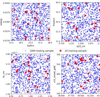
Figure 3.We consider eight uncertain parameter inputs whose ranges are shown as axis limits. The 20 training and 1000 testing data are randomly drawn from the parameter space.
input values. The nodes in each layer are fully connected to all the nodes in its previous and subsequent layers. Each of these connections has an associated weight and bias. A com-plicated NN results in a large number of weights. By tuning these weights and biases based on some training data, we improve the NN approximation of the underlying simulation model.
NN uses the stochastic gradient descent (SGD) method to optimize its weights and biases (Bottou, 2012). SGD opti-mizes variables by minimizing some loss function based on the function’s gradients to these variables. The loss function is usually defined as the mean squared error (MSE) between the NN predictions and model simulations for the same set of model parameter samples in the training data. SGD iter-atively updates the optimized variables at the end of each training epoch. In the process, the learning rate, which spec-ifies how aggressively the optimization algorithm jumps be-tween iterations, greatly affects the algorithm’s performance and has to be tuned. A small learning rate will take a long time to reach the optimum, causing a slow convergence, whereas a big learning rate will bounce around the optimum, causing unstable results and a difficult convergence. Using SGD to optimize a complex NN with many weights requires
a great amount of computational effort and has difficulty in convergence. First, many training data are required to tune a large number of weights. Small training data can easily cause overfitting; i.e., the NN “perfectly” fits the training data but performs badly on new data, thus deteriorating the NN prediction accuracy. In addition, a large number of weights involves massive matrix calculations in evaluating the loss function, slowing down the training process. Furthermore, a complicated NN has difficulty in convergence and can easily get stuck in local minima. In this work, we use SVD to reduce the model output dimensions so as to decrease the number of nodes in the output layer and simplify the NN architecture, thus reducing the size of the weights, enabling a reasonable NN training from small training data, and ultimately improv-ing the computational efficiency.
2.2.3 Bayesian algorithms for NN hyperparameter optimization
a high-performing NN. This requires optimizing an objec-tive functionf (x)over a tree-structured configuration space
x∈X, where some leaf variables (e.g., the number of nodes in the third hidden layer of an NN) are only well defined when branch variables (e.g., a discrete choice of how many layers to use) take particular values. In addition, the opti-mization not only optimizes discrete and continuous vari-ables, but also simultaneously chooses which variables to op-timize. When the NN is used for surrogate modeling, the ob-jective function is the NN accuracy of predicting some val-idation data. In this case, thef (x) does not have a simple closed form but can be evaluated at any arbitrary query point
x in the configuration space. For such an optimization prob-lem, a sequential search method is needed, in addition to in-efficient grid search and random search approaches (Bergstra and Bengio, 2012). The sequential search method starts with some random points in the search space and then iteratively evaluates new points based on NN predictions of previously evaluated points. AfterNevaluations, we choose the optimal combination of the hyperparameters resulting in the highest NN prediction accuracy. Among the sequential search algo-rithms, Bayesian optimization is able to take advantage of full information provided by the history of the optimization to improve the search efficiency.
Bayesian optimization first prescribes a prior belief over the possible objective functions and then sequentially up-dates this prior distribution to posterior distributions as points are evaluated via Bayesian posterior updating. The prior and posterior distributions are the probabilistic model that ap-proximates the unknown objective function we are optimiz-ing. With this probabilistic model, we can sequentially in-duce an acquisition function that leverages the uncertainty in the posterior to guide exploration of new data points for up-dating the model. The acquisition function evaluates the util-ity of candidate points for the next evaluation of f (x), and therefore the next iteration pointxn+1 is selected by maxi-mizing the acquisition function. As more data information is incorporated to exploit the objective function, we get closer to finding the best estimate of the optimizer.
Dependent on the choice of the probabilistic model, we have different Bayesian optimization algorithms (Shahriari et al., 2016). The Gaussian process approach, using the Gaus-sian process as a probabilistic model and expected improve-ment as an acquisition function, has been widely used for pa-rameter optimization (Bardenet and Kegl, 2010; Niranjan et al., 2010). However, this approach has a few disadvantages when applying it to optimize NN hyperparameters. First, it does not work well for categorical variables such as the type of activation functions in NN. Secondly, it selects a new set of parameter points based on the best evaluation data. How-ever, NN usually involves randomization during the train-ing process. So, runntrain-ing NN with the same parameter values can lead to different performance, which suggests that our best point could be just lucky output for the specific setting of randomness. Thirdly, the Gaussian process itself involves
several hyperparameters such as the kernel of the covariance function; a good choice of these hyperparameters can sig-nificantly affect the optimization, but the selection of them is difficult. Lastly, the calculation of the Gaussian process is rather slow, especially for a large number of parameter searches (Snoek et al., 2012).
In this work, we use a tree-structured Parzen estimator (TPE) for NN hyperparameter optimization (Bergstra, et al., 2013). TPE first performs a few iterations of random search, and then it divides collected parameter points into two groups. The first group contains points that give the best scores after evaluation, which can be the top 10 %–25 % of all the points, and the second group has all other points. Next, TPE finds a set of parameters that are more likely to be in the first group and less likely to be in the second group through the following steps: (1) estimate the likelihood probability for each of the two groups based on Parzen window den-sity estimators (Archambeau et al., 2006); (2) sample a bunch of candidate points using the likelihood probability from the first group; and (3) select the point having the largest prob-ability ratio of being in the first group to the second group as the next iteration point. Lastly, we continue the searching until we hit the maximum evaluation and choose the optimal parameter combination that gives the best NN accuracy on the validation data.
The TPE algorithm exhibits significant improvement over classic hyperparameter optimization methods. TPE works well for all types of NN hyperparameter variables; it consid-ers a set of top parametconsid-ers to avoid the influence of NN ran-domization, its implementation is straightforward and has no associated hyperparameters for specification, and the calcu-lation of TPE is computationally fast (Bergstra et al., 2011).
3 Results
In this section, we present the results of building the sur-rogate system of 42 660 GPP variables for sELM. First, we demonstrate that our method using SVD can efficiently build and evaluate a large surrogate system by comparing the re-sults with and without application of SVD. We then inves-tigate the influence of NN’s architecture on surrogate per-formance and show that our method using hyperparameter optimization can quickly generate an accurate NN. Last, we evaluate surrogate accuracy on large-scale spatial and tem-poral GPPs.
The validation data are chosen as 0.3 fractions of the train-ing data. The NN model will not train on the validation data but evaluate the loss function on them at the end of each epoch. In each epoch, the training data are shuffled, and the validation data are always selected from the last 0.3 frac-tion. Precisely, we only use 14 samples to tune NN weights. Attributed to shuffling, these 14 samples can be a different subset from the 20 training data in each epoch, and thus we sufficiently explore the limited 20 data for building the sur-rogates. We use 1000 test data (Fig. 3) to evaluate the NN prediction accuracy, which makes a reasonable assessment of our proposed method within an affordable computational cost. Note that the 1000 test data are not needed for build-ing the surrogates but are used to demonstrate the effective-ness and efficiency of our method. When using our method to build the surrogates of the 42 660 GPPs, only 20 sELM model simulations are used.
We define the loss function as the mean squared error (MSE) between the NN predictions and the sELM simula-tions based on the parameter samples for training. We use Adam algorithm (Kingma and Ba, 2015) for stochastic opti-mization of NN and run it for 800 epochs to minimize the loss function and update NN weights. Adam has been shown as a superior stochastic optimization algorithm in training NN (Basu et al., 2018). There is no right answer for the optimal number of epochs. A small number of epochs could result in underfitting and a large number of epochs may lead to over-fitting. Here we consider a large number of epochs and in the meantime use early stopping to avoid overfitting. During the training, when there is no improvement of loss functions for the validation data in 100 epochs, we stop the training and choose the weights at the epoch resulting in the smallest loss function of the validation data as the optimal weights and the associated NN as the best-trained NN under the given setting. We then use the trained NN to predict the 1000 test data and compare the predictions with the corresponding sELM simulation results to evaluate the NN accuracy. We define two metrics for evaluation: the MSE and the coefficient of determination. The MSE computes the expected value of the squared prediction errors; the smaller the MSE value, the better the prediction. The coefficient of determination, also calledR2score, measures how well the unobserved data are likely to be predicted by the NN model. Denotingyiˆ as the NN prediction of theith sample andyi as the corresponding sELM simulation, theR2score estimated overNssamples is defined asR2=1−
PNs i=1(yi− ˆyi)2
PNs i=1(yi−yi)2
, wherey= 1 Ns
PNs
i=1yi. The
best possible value of R2is 1.0, indicating that the NN can perfectly predict the test data. TheR2score can be negative, indicating the model is arbitrarily poor. A constant model gets an R2 score of 0.0. Compared to MSE, theR2 score considers the variability of the data, which provides a more reasonable measure.
3.1 SVD reduces data dimensionality and improves surrogate efficiency
We consider two scenarios when building the surrogate sys-tem of the 42 660 GPP outputs: Case I involves building the surrogates of reduced data after SVD, and Case II involves building the surrogates of all GPPs directly. In Case I, we first apply SVD to reduce the training data dimensionality, then build surrogates of the singular value coefficients, and last transfer the surrogate system back to the original QoIs (i.e., the 42 660 GPP variables).
The goal of this study is to develop a surrogate method that builds an accurate surrogate system with small training data to reduce the computational costs of simulating expen-sive ESMs. To demonstrate the effectiveness and efficiency of our method, we compare the surrogate performance of the two cases in predicting the 1000 test data from two aspects: (1) for the same number of training data, the predictive ac-curacy of the two surrogates, and (2) the number of training data used to achieve similar predictive accuracy.
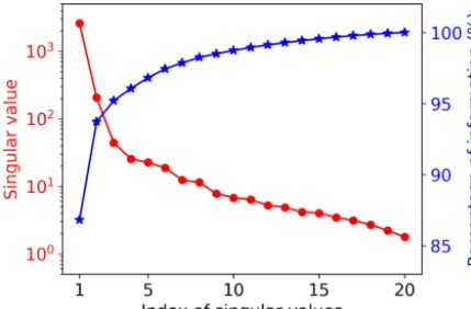
Figure 4 shows the singular value decay of decomposi-tion of the training data matrix having 20 samples and 42 660 GPP variables. The figure indicates that the singular values decay very fast. The first two singular values drop about 1 magnitude, and the first five singular values can capture 97 % of the information from the training data matrix. To choose a suitable number of singular value coefficients (Nsvd) to com-press the training data and build a surrogate for, we consider a series of Nsvds, whereNsvd=1, 5, 10, 15, and 20, and in-vestigate their impact on NN performance. To make a fair comparison, the same NN architectures are used for allNsvd cases. We consider a simple NN with two hidden layers, and each hidden layer has 10 nodes. Figure 5 shows the predic-tion performance of the NNs based on the 20 training data. The figure indicates that with consideration of only one sin-gular value coefficient, the averaged MSE of the predictions is about 0.053, and the NN model can fit the sELM simula-tion data well with theR2score of 0.83. When five singular value coefficients are considered, the NN prediction accuracy improves with the MSE of 0.02 and theR2 score of 0.93. AfterNsvd=5, the MSE andR2score have minor changes, suggesting that for the limited 20 training data,Nsvd=5 is a good choice to compress the GPPs and build a surrogate for. At this time, the surrogate error becomes dominant compared to the SVD approximation error, and including more than five singular value coefficients would barely improve the NN prediction unless more training data are included to reduce the surrogate error. In the following, we considerNsvd=5 in Case I and compare its surrogate prediction performance with Case II, which builds surrogates for all GPPs directly.
Figure 4. Singular value decay and the information contained in the first largest singular values. The top five singular values contain 97 % of the information from the training data matrix with 42 660 GPP variables and 20 samples.
Figure 5.Performance of the NNs trained by 20 data with consid-eration of the different number of singular value coefficients after SVD.
of the five singular value coefficients are plotted. The figure indicates that the loss functions of the two datasets have sim-ilar decay, decreasing dramatically at the first 10 epochs and then slowly decreasing to the end of training. The closely overlapped two lines in Fig. 6a suggest that the trained NN captures the relationship between sELM inputs and outputs pretty well and can give reasonable predictions of GPPs for a given parameter sample.
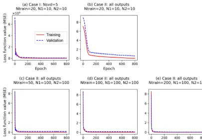
To make a fair comparison, we use the same NN architec-ture in Case II as in Case I except that the output layer of NN in Case II has all 42 660 GPPs and the output layer in Case I has only five singular value coefficients. Figure 6b indicates that the simple NN with 20 hidden nodes is not sophisticated enough to capture the complex relationship between the eight inputs and 42 660 outputs. As we can see in Fig. 6b, both training and validation losses are relatively high, suggesting an underfitting. The validation loss is always larger than the training loss, suggesting that the fitted NN does not gener-alize well and may result in poor performance in predicting new data. Figure 7 showsR2scores of Case II in predicting
the 1000 test data. The figure indicates that the simple NN trained by 20 data in Case II has a very poor prediction accu-racy with theR2score of only 0.05, close to a constant model performance with a zeroR2score. However, with the same NN trained by the same 20 data, our SVD-based surrogate method can achieve a high prediction accuracy with theR2
score of 0.93. This demonstrates our method’s capability of using a few training samples to build an accurate surrogate model, greatly reducing the computational costs of generat-ing expensive model simulation data.
On the other hand, the poor performance in Case II sug-gests that a wider and deeper NN is needed when we con-sider the large outputs directly. We thus increase the number of nodes in each hidden layer to 100 and use this complex NN with a total of 200 hidden nodes to approximate the relation-ship of the eight inputs and 42 660 outputs in Case II. This complex NN dramatically increases its number of parame-ters (including weights and biases) to 4.3 million from 255 in Case I. To fit this wide NN and calibrate its large parameters, 20 training data are too few to get a reasonable fit. No matter how we adjust the NN hyperparameters, we cannot get a sta-ble solution in training. We then increase the number of train-ing data to 50, and Fig. 6c shows that the increased number of data greatly decreases the training and validation losses; the validation loss is slightly higher than the training loss, imply-ing a good fit. Figure 7 indicates that the complex NN with 200 hidden nodes trained by 50 data in Case II significantly improves the prediction accuracy with theR2score of 0.73. However, Case II’s predictive performance is still worse than Case I, which has theR2score of 0.93. We keep increasing the number of training data (Ntrain) to 100 and 200 in Case II. Figure 6d and e indicate that the increase in the number of training data brings the validation loss closer and closer to the training loss, making the fitted NN represent the underlying sELM better and better. Figure 7 shows that the nicely fitted NNs trained by large Ntrains lead to a high prediction accu-racy. WithNtrain=100, theR2score is about 0.89, and with
Ntrain=200, theR2score is up to 0.95. However, compared to Case I using 20 training data to get a predictiveR2score of 0.93, Case II uses nearly 200 data to get similar accuracy, increasing the computational costs 10-fold. Note that each training data point involves one sELM simulation, and one regional sELM run takes about 24 h on one processor. Thus, our SVD-based surrogate method greatly improves compu-tational efficiency in accurate surrogate modeling.
Figure 6.Changes of loss function values along epochs for training and validation data(a)in Case I, which builds surrogates of the five singular value coefficients with a simple NN (two hidden layers; each layer has 10 nodes,N1=N2=10) based on 20 training data (Ntrain=
20), and(b–e)in Case II, which builds surrogates of all outputs with different NN architectures and different training data size.
Figure 7.Comparison of NN performance between Case I (building surrogates of five singular value coefficients after SVD based on 20 training data;Nsvd=5; red dashed line) and Case II (building surrogates for all outputs directly with different numbers of training data; red solid line). Each training data point represents one sELM simulation. The rightyaxis shows the time in training the NN in Case II. The time for training the NN in Case I is 4 s.
time leads to high computational costs in NN hyperparame-ter optimization for which a massive amount of NN training is involved in searching the wide hyperparameter space for a high-performing NN model, as discussed in Sect. 3.2.
3.2 NN’s hyperparameter optimization improves surrogate accuracy
NN has a large number of hyperparameters. Here we adjust five hyperparameters and use Case I to investigate their influence on surrogate prediction accuracy. The five hyper-parameters are the following: the number of hidden layers (L) for which we consider the three most hidden layers; the number of nodes in hidden layer 1 (N1), in hidden layer 2 (N2), and in hidden layer 3 (N3); and the learning rate (lr) of the Adam optimization algorithm. We consider the following choices: L= {2,3}, N1= {10,20,40,60,80,100}, N2= {10,20,40,60,80,100}, N3= {0,10,20,40,60,80,100}, and lr=U[0.001,0.1]. The first four hyperparameters are discrete variables and the last one, lr, is a continuous variable with uniform distribution. The choice of L determines the selection of N3, showing a tree-like structure. We use a tree-structured Parzen estimator (TPE) to search the five-hyperparameter space and find a set of values that gives the best-performing NN. We fix the activation function as ReLU (Agarap, 2018), which has been widely used and shown to produce good NN predictions.
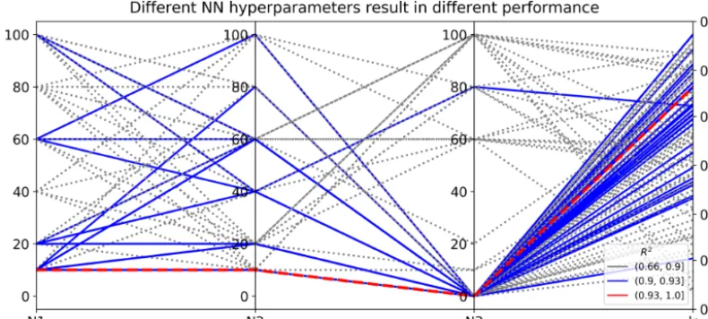
Figure 8.Different sets of NN hyperparameters result in differentR2scores in evaluating the 1000 test data.Nl is the number of nodes in
hidden layerl, wherel=1, 2, and 3; lr is the learning rate of the Adam algorithm for NN weight optimization.
N2=10, N3=0, and lr=0.08 gives the best validation score. To investigate the impact of hyperparameters on NN prediction accuracy, we show the 100 sets of hyperparame-ters and their resultingR2scores in predicting the 1000 test data in Fig. 8. The figure indicates that different hyperparam-eter values result in dramatically different NN performance. The prediction R2 scores range from 0.66 to 0.93, and 32 hyperparameter sets haveR2scores over 0.90. The selected optimal NN producing the smallest MSE on the validation data also gives the best prediction performance on the test data with theR2score of 0.93. It is desired that the best NN model chosen by validation data gives the best predictions; however, in practice it is not always the case, especially when the prediction data deviate a lot from the validation data. Ex-trapolation is always a difficulty in surrogate modeling, and research is ongoing to improve extrapolation accuracy.
Although NNs perform significantly different with a dif-ferent combination of hyperparameters, the TPE algorithm can efficiently find high-performing NNs based on previous sample information. As shown in Fig. 8, good-performing NNs prefer simple architectures with two hidden layers; e.g., most blue lines haveN3of 0. After TPE finds a good archi-tecture ofN1=10 andN2=10, it samples around this archi-tecture in the hyperparameter space to fine tune the learning rate until it finds the most suitable lr of 0.08. This work con-siders five hyperparameters with limited choices; increasing the dimensions and possible choices of the hyperparameters would make the search more thorough and could produce a better-performing NN. Our surrogate method with SVD can accelerate the optimization process by reducing the NN train-ing time.
3.3 Evaluation of surrogate accuracy on large-scale spatial and temporal data
Using only 20 expensive sELM runs, we quickly build an accurate surrogate system of 42 660 GPPs at 1422 locations for 30 years. Therefore, for a data–model integration prob-lem with QoIs within given spatial and temporal ranges, we can directly extract the information of interest from the surro-gate system to advance the analysis. The best-performing NN generated from our method gives an overall accurate predic-tion of the 42 660 GPPs with averaged MSE of 0.02 andR2
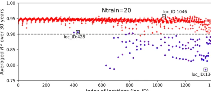
scores of 0.93. When using the subset of the surrogate system for data–model integration studies, it is desired to analyze the surrogate accuracy at individual locations for specific times. Figure 9 shows averagedR2scores over 30 years at 1422 locations. The figure indicates that the surrogate accuracy is not uniformly good for all the locations. We observe that most locations haveR2 scores above 0.9, with the bestR2
score of 0.96, and about 100 locations haveR2scores below 0.90 with the smallestR2score of 0.79. We highlight the lo-cations having zero GPP simulations in blue circles and find that these locations generally have poor predictions with low
R2scores. Referring to Fig. 2, where we label the locations column-wise from south to north and from west to east, we identify the locations with zero GPPs as mostly located in the north where the temperature is relatively low and annual GPPs tend to be zero for parameter samples.
Figure 9.AveragedR2scores over 30 years at 1422 locations in evaluating the 1000 test data based on 20 training samples; the blue circles identify the locations having zero GPP simulations.
Figure 10.Simulations of annual GPPs (g C m−2d−1) from sELM and the NN-based surrogate model in evaluating 1000 test data for 30 years at three locations, with the NN trained by 20 data using our method.
GPP data. At location 1046 where the annual GPPs are rela-tively high with positive values, NN produces a great fit with a highR2score of 0.96 and a small MSE of 0.013. Location 1046 (Fig. 2) is close to the lake where the variance in atmo-spheric drivers (e.g., temperature) is moderated. This reduced variance leads to a smooth response surface of GPP for which NN can easily build an accurate surrogate. In contrast, loca-tion 1345 has a large number of simulated GPPs less than 1.0, including many zero GPPs. NN shows difficulty in predicting these small GPPs, resulting in a relatively poor performance with theR2score of 0.79. Location 1345 is in the north and has the lowest mean annual temperature, so most parameter samples cause low vegetation growth and small GPP values. Moreover, location 1345 is far away from the lakes and has a large variation in atmospheric drivers. Since this location has a climate that is at the extreme end of the range for decidu-ous forests, the model response is expected and reasonable. However, this leads to a strong nonlinear response surface that leads to difficulty in surrogate modeling. In comparison, although location 428 is in the north with some small GPPs including zero values, it is also close to the lake, which has a
small variance in atmospheric drivers. Thus, the NN predic-tion performance in locapredic-tion 428 is not bad with theR2score of 0.91.
Figure 11 plots the averagedR2scores over all locations for 30 years. TheR2scores have small fluctuations between 0.93 and 0.94, displaying a uniformly good fit among the simulated years. So, when using the surrogate model at any specific year for a data–model analysis, we should be able to obtain a good approximation. In this study, we are con-sidering annual GPPs. Although the variation of atmospheric drivers between years has an impact on surrogate accuracy, its influence is less strong compared to monthly GPPs, so a uniformly good fit among years is expected.
Figure 11.AveragedR2scores over 1422 locations at 30 years in evaluating the 1000 test data.
strong nonlinear and discontinuous problems, one strategy is using physics-informed domain decomposition methods to build surrogate models separately in different response sur-face regimes. This strategy requires the surrogate methods to be strongly connected to the simulation model, and the methods are generally problem-specific, requiring expert in-teraction. Another strategy is increasing the number of train-ing data to explore complex problems. This strategy requires an increase in computational costs for expensive model sim-ulations. In the following Sect. 4, we investigate these two strategies and discuss their influence on surrogate accuracy.
4 Discussion
ESMs are complex, with response surfaces that always dis-play strong nonlinearity and discontinuity, creating a chal-lenge for surrogate modeling. In this section, we consider the strategies of physics-informed learning and an increase in the number of training data to improve surrogate accuracy. We conduct two corresponding experiments to investigate our method’s performance in the application of these two strate-gies. In experiment I, we divide the parameter space into two parts, producing zero GPPs and nonzero GPPs, and we use 20 training data to build surrogates of the 42 660 GPPs in the regime, generating nonzero GPP samples. In experiment II, we build the surrogates of the 42 660 GPPs in the original parameter domain (Fig. 3) but with an increasing number of training data (200 and 1000).
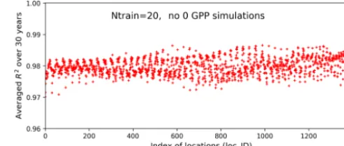
We use the results of Case I as a baseline to investigate our method’s performance in the two experiments. Figure 12 shows averagedR2scores over 30 years at the 1422 locations in experiment I. The figure indicates that without zero GPPs our method can produce a very accurate surrogate at all lo-cations with a uniformly highR2score of 0.98. Building the surrogates in the subdomain without zero GPPs not only sig-nificantly improves the prediction accuracy in locations orig-inally having a poor fit in Case I, but also further improves the prediction accuracy in locations that already have a good fit in Case I. For example, theR2score is dramatically
im-Figure 12.AveragedR2scores over 30 years at 1422 locations in evaluating the 1000 test data based on 20 training data in experi-ment I in which the samples are generated in a subdomain of the parameter space without zero GPP simulations. The averagedR2
score is 0.98.
proved from 0.79 to 0.97 at location 1345, from 0.96 to 0.99 at location 1046, and from 0.91 to 0.98 at location 428. As shown in Fig. 13, the NN almost perfectly reproduces sELM simulations at these three locations. Experiment I indicates that physics-informed domain decomposition can be a good strategy to improve surrogate accuracy. For smooth problems (e.g., no sharp jumps from nonzeros to zeros in response sur-faces), our method can build a very accurate surrogate model based on a few training data.
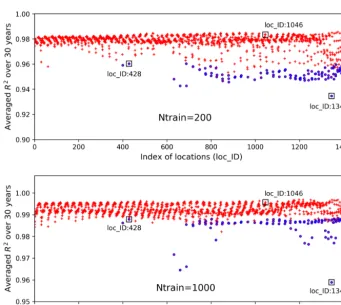
Figure 14 shows averagedR2scores over 30 years at 1422 locations based on 200 and 1000 training data in experi-ment II. The figure indicates that an increase in the num-ber of training data greatly enhances NN prediction accuracy. Adding 10-fold additional data fromNtrain=20 toNtrain= 200, the overallR2 score improves from 0.93 to 0.98; fur-ther increasingNtrainto 1000, the averagedR2score is up to 0.993 with the worst value of 0.96. Although we observe sim-ilar nonuniform performance among locations in Fig. 14 as in Fig. 9, where the locations with zero GPPs have smallerR2
scores than others, increasing Ntrain significantly improves the accuracy at all locations, especially those originally hav-ing poor fits in Case I. For example, whenNtrain=200, most blue-circled locations have R2 scores above 0.95, and for
Ntrain=1000, theR2 scores at these blue-circled locations are above 0.985 in comparison to the values below 0.9 when
train-Figure 13.Simulations of annual GPPs (g C m−2d−1) from sELM and the NN-based surrogate model in evaluating 1000 test data for 30 years at three locations in experiment I in which the samples are generated in a subdomain of the parameter space without zero GPP simulations.
Figure 14.AveragedR2scores over 30 years at 1422 locations in evaluating the 1000 test data based on 200 and 1000 training samples; the blue circles identify the locations having zero GPP simulations.
ing data and greatly improves prediction accuracy asNtrain increases.
The analysis of the two experiments suggests that our method is data-efficient for continuous problems. To improve the surrogate accuracy in discontinuous and highly nonlinear problems, we can use the physical-informed domain decom-position to focus on the continuous and smooth regions of the response surface. If the discontinuity is the inherent feature
of the underlying function for which we need a surrogate, an increase in the number of training data would be a good solution for surrogate accuracy improvement.
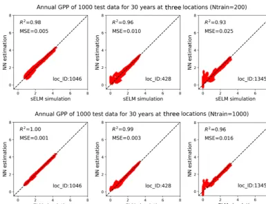
Figure 15.Simulations of annual GPPs (g C m−2d−1) from sELM and the NN-based surrogate model in evaluating 1000 test data for 30 years at three locations, with the NN trained by 200 and 1000 data.
and temporal GPP variables, as well as for parameter opti-mization and uncertainty quantification based on single-site, multiple-site, single-year, or multiple-year GPP observations using any defined objective functions. In addition, with the newly collected observations from additional sites or further time periods, we can use the same surrogate system for anal-ysis as long as the QoIs are within the surrogate simulation ranges. In a future study, we will pursue data–model integra-tion using the constructed surrogate system.
5 Conclusions
In this work, we develop an SVD-enhanced, Bayesian-optimized, and NN-based surrogate method to improve the computational efficiency of large-scale surrogate modeling to advance model–data integration studies in Earth system model simulations. Our method is data-efficient in that only 20 model simulations are needed to build an accurate sur-rogate system. This is a promising result because large Earth system model ensembles are always computationally infeasi-ble, and 20 is a reasonable and affordable number of simula-tions to consider. In addition, our method is general purpose and can be efficiently applied to a wide range of Earth sys-tem problems with different spatial scales (local, regional, or global) for different simulation periods. It is supereffective
for smooth problems and scaled well for highly nonlinear and discontinuous problems.
We apply our surrogate method to a regional ecosystem model. The results indicate that using only 20 model runs, we can build an accurate surrogate system of 42 660 spatially and temporally varied GPPs with theR2score of 0.93 and MSE of 0.02. For locations with robust vegetation growth across the ensemble, our method can almost perfectly pre-dict the model simulations with theR2 score of 0.96. For locations with low vegetation growth for some parameter samples and large variation in atmospheric drivers that cause discontinuous response surfaces, using physics-informed do-main decomposition or an increase in the number training samples, our method can produce accurate predictions with theR2 scores of 0.97 and 0.96, respectively. This applica-tion demonstrates our method’s capability to accurately re-produce expensive model simulations based on a few parallel model runs.
machine-learning techniques can be provided upon request via [email protected].
Data availability. All the data used in this study are model simula-tion data, which can be generated by running the sELM.
Author contributions. DL developed the methods and carried them out. DR developed the model code and performed the model simu-lations. DL prepared the paper with contributions from the coauthor.
Competing interests. The authors declare that they have no conflict of interest.
Acknowledgements. Primary support for this work was provided by the Scientific Discovery through Advanced Computing (SciDAC) program, funded by the U.S. Department of Energy (DOE), Office of Advanced Scientific Computing Research (ASCR) and Office of Biological and Environmental Research (BER). Additional support was provided by BER’s Terrestrial Ecosystem Science Scientific Focus Area (TES-SFA) project. The authors are supported by Oak Ridge National Laboratory, which is supported by the DOE under contract DE-AC05-00OR22725.
Review statement. This paper was edited by David Topping and re-viewed by Tianfang Xu and Xiankui Zeng.
References
Agarap, A. F. M.: Deep learning using Rectified Linear Units (ReLU), https://arxiv.org/pdf/1803.08375 (last access: 7 Febru-ary 2019), 2018.
Archambeau, C., Valle, M., Assenza, A., and Verleysen, M.: Assessment of probability density estimation meth-ods: Parzen window and finite Gaussian mixtures, IEEE, ISCAS 2006, 21–24 May 2006, Island of Kos, Greece, https://doi.org/10.1109/ISCAS.2006.1693317, 2006.
Bardenet, R. and Kegl, B.: Surrogating the surrogate: accelerat-ing Gaussian-process-based global optimization with a mixture cross-entropy algorithm, in: International Conference on Ma-chine Learning, 21–24 June 2010, Haifa, Israel, 55–62, 2010. Basu, A., De, S., Mukherjee, A., and Ullah, E.: Convergence
guarantees for rmsprop and adam in nonconvex optimization and their comparison to nesterov acceleration on autoencoders, arXiv preprint arXiv:1807.06766, available at: https://arxiv.org/ abs/1807.06766 (last access: 10 March 2019), 2018.
Bergstra, J. and Bengio, Y.: Random search for hyper-parameter op-timization, J. Mach. Learn. Res., 13, 281–305, 2012.
Bergstra, J. S., Bardenet, R., Bengio, Y., and Kegl, B.: Algorithms for hyperparameter optimization, NIPS, 24, 2546–2554, 2011. Bergstra, J. S., Yamins, D., and Cox, D. D.: Hyperopt: A Python
library for optimizing the hyperparameters of machine learning
algorithms, in: Proceedings of the 12th Python in Science Con-ference, 24–29 June 2013, Austin, Texas, USA, 13–20, 2013. Bilionis, I., Drewniak, B. A., and Constantinescu, E. M.: Crop
phys-iology calibration in the CLM, Geosci. Model Dev., 8, 1071– 1083, https://doi.org/10.5194/gmd-8-1071-2015, 2015.
Bottou, L.: Stochastic gradient descent tricks, Neural networks: tricks of the trade: 2nd edition, Springer Berlin Heidelberg, Ger-many, 2012.
Fox, A., Williams, M., Richardson, A. D., Cameron, D., Gove, J. H., Quaife, T., Ricciuto, D., Reichstein, M., Tomelleri, E., Trudinger, C. M., and Van Wijk, M. T.: The REFLEX project: Comparing different algorithms and implementations for the inversion of a terrestrial ecosystem model against eddy covariance data, Agr. Forest Meteorol., 149, 1597–1615, 2009.
Gong, W., Duan, Q., Li, J., Wang, C., Di, Z., Dai, Y., Ye, A., and Miao, C.: Multi-objective parameter optimization of common land model using adaptive surrogate modeling, Hydrol. Earth Syst. Sci., 19, 2409–2425, https://doi.org/10.5194/hess-19-2409-2015, 2015.
Huang, M., Ray, J., Hou, Z., Ren, H., Liu, Y., and Swiler, L.: On the applicability of surrogate-based Markov chain Monte Carlo-Bayesian inversion to the Community Land Model: Case studies at flux tower sites, J. Geophys. Res.-Atmos., 121, 7548–7563, https://doi.org/10.1002/2015JD024339, 2016.
Kim, H.: Global Soil Wetness Project Phase 3 Atmospheric Bound-ary Conditions (Experiment 1). Data Integration and Analysis System (DIAS), https://doi.org/10.20783/DIAS.501, 2017. Kingma, D. P. and Ba, J.: Adam: a Method for Stochastic
Opti-mization, International Conference on Learning Representations, 7–9 May 2015, San Diego, CA, USA, 1–13, 2015.
Lu, D., Ricciuto, D., Walker, A., Safta, C., and Munger, W.: Bayesian calibration of terrestrial ecosystem models: a study of advanced Markov chain Monte Carlo methods, Biogeosciences, 14, 4295–4314, https://doi.org/10.5194/bg-14-4295-2017, 2017. Lu, D., Ricciuto, D., Stoyanov, M., and Gu, L.: Calibra-tion of the E3SM land model using surrogate-based global optimization, J. Adv. Model. Earth Syst., 10, 1337–1356, https://doi.org/10.1002/2017MS001134, 2018.
Luo, J. and Lu, W.: Comparison of surrogate models with different methods in groundwater remediation process, J. Earth Syst. Sci., 123, 1579–1589, 2014.
Müller, J., Paudel, R., Shoemaker, C. A., Woodbury, J., Wang, Y., and Mahowald, N.: CH4parameter estimation in CLM4.5bgc
us-ing surrogate global optimization, Geosci. Model Dev., 8, 3285– 3310, https://doi.org/10.5194/gmd-8-3285-2015, 2015.
Niranjan, S., Krause, A., Kakade, A., and Seeger, M.: Gaussian pro-cess optimization in the bandit setting: No regret and experimen-tal design, in: Proceedings of the 27th International Conference on Machine Learning, 21–24 June 2010, Haifa, Israel, 2010. Oleson, K. W. and Lawrence, D. M.: Technical description
of version 4.5 of the Community Land Model (CLM). NCAR Tech. Note NCAR/TN-5031STR, 420 pp., National Center for Atmospheric Research, Boulder, CA, USA, https://doi.org/10.5065/D6RR1W7M, 2013.
Razavi, S., Tolson, B. A., and Burn, D. H.: Review of surrogate modeling in water resources, Water Resour. Res., 48, W07401, https://doi.org/10.1029/2011WR011527, 2012.
Ricciuto, D.: simple_ELM, available at: https://github.com/ dmricciuto/OSCM_SciDAC/tree/master/models/simple_ELM, last access: 29 March 2019.
Ricciuto, D., Sargsyan, K., and Thornton, P.: The impact of para-metric uncertainties on biogeochemistry in the E3SM land model, J. Adv. Model. Earth Syst., 10, 297–319, 2018.
Sargsyan, K., Safta, C., Najm, H. N., Debusschere, B., Ricciuto, D. M., and Thornton, P. E.: Dimensionality reduction for complex models via Bayesian compressive sensing, Int. J. Uncert. Quant., 4, 63–93, 2014.
Shahriari, B., Swersky, K., Wang, Z., Adams, R. P., and de Freitas, N.: Taking the Human Out of the Loop: A Re-view of Bayesian Optimization, Proc. IEEE, 104, 148–175, https://doi.org/10.1109/jproc.2015.2494218, 2016.
Snoek, J., Larochelle, H., and Adams, R. P.: Practical Bayesian op-timization of machine learning algorithms, in: 26th Annual Con-ference on Neural Information Processing Systems, 3–8 Decem-ber 2012, Lake Tahoe, Nevada, USA, 2960–2968, 2012. Viana, F. A., Simpson, T. W., Balabanov, V., and Toropov, V.:
Meta-modeling in multidisciplinary design optimization: How far have we really come?, AIAA J., 52, 670–690, 2014.
Williams, M., Schwarz, P. A., Law, B. E., Irvine, J., and Kurpius, M.: An improved analysis of forest carbon dynamics using data assimilation, Glob. Change Biol., 11, 89–105, 2005.