University of New Orleans University of New Orleans
ScholarWorks@UNO
ScholarWorks@UNO
University of New Orleans Theses and
Dissertations Dissertations and Theses
5-20-2005
Design and Implementation of an Universal Lattice Decoder on
Design and Implementation of an Universal Lattice Decoder on
FPGA
FPGA
Swapna Kura
University of New Orleans
Follow this and additional works at: https://scholarworks.uno.edu/td
Recommended Citation Recommended Citation
Kura, Swapna, "Design and Implementation of an Universal Lattice Decoder on FPGA" (2005). University of New Orleans Theses and Dissertations. 236.
https://scholarworks.uno.edu/td/236
This Thesis is protected by copyright and/or related rights. It has been brought to you by ScholarWorks@UNO with permission from the rights-holder(s). You are free to use this Thesis in any way that is permitted by the copyright and related rights legislation that applies to your use. For other uses you need to obtain permission from the rights-holder(s) directly, unless additional rights are indicated by a Creative Commons license in the record and/or on the work itself.
DESIGN AND IMPLEMENTATION OF AN UNIVERSAL LATTICE DECODER ON FPGA
A Thesis
Submitted to the Graduate Faculty of the University of New Orleans
in partial fulfillment of the requirements for the degree of
Master of Science in
The Department of Electrical Engineering
by
Swapna Kura
B.Tech J.N.T.U, 2001
ACKNOWLEDGEMENTS
I would like to express my special thanks to Dr. Jing Ma for being my advisor throughout
my thesis research. I appreciate her patience, guidance and supervision of my work which helped
me in progressing in right path.
I acknowledge Dr. Bhaskar Kura for his support throughout my graduate program
without which it would have been impossible for me to get thru my master’s degree. His
patience, guidance and insight served as invaluable assets in both my personal and academic
lives.
I would also express my sincere thanks to Dr. Xinming Huang and Dr. Edit Bourgeois for
their willingness to serve as members in my thesis committee.
I would express my heartfelt thanks to my parents and all family members. Their
blessings and love were always with me and encouraged me in stepping forward in life.
I would thank my colleagues for being eager and prompt enough to help me when I
needed them. Finally, I would like to thank all my friends and cousins for their encouragement
GLOSSARY OF ABBREVIATIONS
MIMO – Multiple Input Multiple Output
FPGA – Field Programmable Gate Arrays
PLD – Programmable Logic Device
ASIC – Application Specific Integrated Circuit
IC – Integrated Chip
SOC – System-On-Chip
FSM – Finite State Machine
AWGN – Additive White Gaussian Noise
PAM – Pulse Amplitude Modulation
BER – Bit Error Rate
ML – Maximum Likelihood
DSP – Digital Signal Processor
VHDL – Very High speed integrated Description Language
RTL – Register Transfer Level
TABLE OF CONTENTS
LIST OF FIGURES...vi
LIST OF TABLES………vii
ABSTRACT………...viii
1 INTRODUCTION... 1
1.1 Motivations and Background... 1
1.2 Research Objective ... 4
1.3 Contribution of Thesis ... 4
1.4 Organization of Thesis... 5
2 FPGAs and MIMO Channels ... 6
2.1 MIMO Channels... 6
2.2 Field Programmable Gate Array (FPGA)... 8
3 Sphere Decoding Algorithm... 11
3.1 The Sphere Decoder ... 11
3.1.1 Maximum-Likelihood Criterion... 12
3.1.2 ML Decoding In Sphere Decoder ... 13
3.2 Flow-Chart... 14
3.2.1 Pre-Processing... 15
3.2.2 Decoding... 15
3.3 Decoding Procedure ... 18
3.4 High Level Simulation of the Sphere Decoding Algorithm... 19
3.5 Decoder Architecture Scheduling... 20
3.5.1 Data Flow of the Algorithm... 22
3.5.2 FSM Design ... 25
3.6 Simulation Results... 27
3.6.1 Non-Restoring Square Root Algorithm ... 27
4 Improved Sphere Decoding Algorithm ... 30
4.1 Improved Sphere Decoding Algorithm ... 30
4.1.1 Derivation of Modifications... 31
4.1.2 Flow-Chart ... 35
4.2 Decoding Procedure ... 36
4.3 High Level Description of the improved Sphere decoder ... 37
4.4 Decode Architecture Scheduling... 38
4.6 Simulation Results... 42
4.7 Data Dependency... 43
5 FPGA Based Architecture Design... 46
5.1 Lattice Decoder Architecture... 46
5.2 Parallel Structure ... 47
5.3 VLSI Design Flow... 52
5.4 Design Optimization... 54
6 RESULTS... 57
6.1 Experimental Setup... 57
6.2 Pre-Processing Results ... 57
6.3 Decoding Results... 58
6.3.1 Simulation Results ... 58
6.3.2 Synthesis Results ... 60
6.3.3 Decoding Rate... 62
6.3.4 BER Performance ... 67
6.3.5 Comparison between FPGA and DSP Implementations ... 68
6.4 Conclusions ... 70
REFERENCES...………...72
LIST OF FIGURES
Figure 2.1: A MIMO system. (a) MIMO Transmitter. (b) MIMO receiver ... 7
Figure 2.2: Virtex-II FPGA architecture [Chris] ... 10
Figure 3.1: Flowchart of a Sphere decoding algorithm [Viterbo 1999] ... 14
Figure 3.2: Flowchart of a Sphere decoding algorithm showing states... 22
Figure 3.3: Input and Output pins for original sphere decoder... 24
Figure 3.4: The FSM diagram of Sphere decoding algorithm ... 26
Figure 4.1: Flow chart of improved algorithm... 35
Figure 4.2: Flow chart of an improved algorithm showing states ... 39
Figure 4.3: Input and Output pins for improved sphere decoder... 40
Figure 4.4: Overview of the complete system ... 42
Figure 4.5: Dependency graph of the Sphere decoding algorithm ... 43
Figure 5.1: The hardware architecture of improved sphere decoding algorithm... 46
Figure 5.2: The hardware architecture of parallel-pipeline improved sphere decoding algorithm ... 48
Figure 5.3: An example of improved sphere decoding algorithm (a) Sequential implementation (b) Parallel-Pipeline implementation ... 49
Figure 5.4: Design flow for an FPGA... 52
Figure 5.5: Workspace of Project Navigator ... 53
Figure 5.6: RTL schematic of parallel-pipeline implemented sphere decoder generated by Xilinx ISE 6.2i ... 56
Figure 6.1: Bar chart showing the simulations times of each states in both algorithms... 59
Figure 6.2: Xilinx Virtex-II 1000 FPGA Device Description ... 61
LIST OF TABLES
Table 3.1: Pin descriptions for the decoder controller of the original sphere decoding algorithm
... 25
Table 3.1: Simulation Times of each state in original algorithm ... 27
Table 4.1: Pin descriptions for the decoder controller of the improved sphere decoding algorithm ... 41
Table 4.2: Simulation Times of each state in improved algorithm ... 43
Table 5.1: Sequence of states for an example of improved algorithm at 6dB SNR... 48
Table 6.1: Average number of state visits in sequential implementation at 20 dB... 60
Table 6.2: Average number of state visits in parallel-pipeline implementation at 20 dB... 60
Table 6.3: Synthesis results of m=n=4 MIMO system ... 61
Table 6.4: Sequence of state in Sequential procedure... 63
Table 6.5: Sequence of state in Parallel-Pipeline procedure... 64
Table 6.6: Comparison of decoding rate at 20 dB... 65
ABSTRACT
In wireless communication, MIMO (multiple input multiple output) is one of the
promising technologies which improves the range and performance of transmission without
increasing the bandwidth, while providing high rates. High speed hardware MIMO decoders are
one of the keys to apply this technology in applications. In order to support the high data rates,
the underlying hardware must have significant processing capabilities. FPGA improves the speed
of signal processing using parallelism and reconfigurability advantages.
The objective of this thesis is to develop an efficient hardware architectural model for the
universal lattice decoder and prototype it on FPGA. The original algorithm is modified to ensure
the high data rate via taking the advantage of FPGA features. The simulation results of software,
hardware are verified and the BER performance of both the algorithms is estimated. The system
prototype of the decoder with 4-transmit and 4-receive antennas using a 4-PAM (Pulse amplitude
modulation) supports 6.32 Mbit/s data rate for parallel-pipeline implementation on FPGA
1 INTRODUCTION
1.1 Motivations and Background
Although wireless technologies have been around for a while, there has been a recent and
rapid surge in the evolution of new standards that enable and accelerate the convergence of
telecommunications and IP networking to provide new multimedia services. To keep up with the
demands of wireless network services, the capacities of systems are increased. The most
brute-force approach to increasing wireless data rate is to use more frequency channels to increase
modulation rate [Jones 2003]. This "channel bonding" approach will not meet the needs of
wireless network consumers for the following reasons: First, while channel bonding increases
data rate, it decreases the transmission range for the same transmit power. Second, channel
bonding robs channels from other systems that operate nearby.
MIMO (multiple input multiple output) antenna technology is considered as one of the
solutions to support the wireless network services. It essentially multiplies data throughput, with
a simultaneous increase in range and reliability, without consuming any extra frequency
spectrum [Jones 2003]. The multi-antenna wireless communication systems are capable of
providing data transmission at potentially very high rates. Furthermore, to secure high reliability
of the data transmission, special attention has to be given to the receiver design. The data streams
are separated at the receiver using algorithms that rely on estimates of all channels between each
transmitter and each receiver. The low complexity suboptimal detection algorithm for MIMO
signals was the Vertical Bell Labs Layered Space-Time (VBLAST) algorithm. This is an
zero-forcing function [Jones 2003]. While the iterative detection can increase receiver sensitivity,
there are substantial problems with a real implementation.
The optimal detection strategy for a MIMO receiver is to perform a maximum-likelihood
search over all possible transmitted symbol sets. ML decoding is equivalent to finding the closest
lattice point to the received point in a lattice constellation. ML detection at the receiver becomes
an essential part in high-performance MIMO communication systems [Burg 2004]. Thus, ML
decoding algorithms and their architecture are active research areas in wireless communication
that motivated the research in MIMO systems.
For decoding the lattices with no regular structure at the receiver follows two main
branches. Pohst [Pohst 1981] in 1981 examined lattice points lying inside a hyper sphere,
whereas Kannan in 1983 used a rectangular parallelepiped. Both methods later appeared in
revised and extended versions. Pohst method is intended as practical tool while Kannan’s is a
theoretical tool. In [Viterbo 1999], a technique referred to as the "sphere decoding" (based on the
Fincke-Pohst algorithm) was proposed for lattice code decoding [Eriksson 2002]. This performs
a bounded distance search among the lattice points falling inside the sphere centered at the
received point.
The sphere decoder provides the maximum-likelihood estimate of the transmitted signal
sequence with complexity comparable, at high signal-to-noise ratios (SNRs), to VBLAST
nulling/canceling algorithm [Bertrand 2003]. It is later stated that sphere decoding often
significantly outperforms heuristic nulling and canceling. Developing an efficient sphere decoder
with reduced complexity has received significant attention due to its applications to wireless
communications as in [Viterbo 1999]. However, most modifications suggested are well suited for
algorithm the front end of the receiver is implemented on FPGA whereas actual decoder function
is implemented on a DSP processor.
As the performance requirements of today’s communication systems are outstripping the
capabilities of general-purpose DSP processors, the need for DSP implementations to seek
hardware solution arises [Dan 2004]. FPGAs provide an ideal platform for DSP implementation,
combining the reprogrammability, architectural flexibility, and support of parallelism.
FPGA-based hardware platforms also meet the critical requirements such as processing speed,
time-to-market, system integration etc. Due to the significant processing capabilities of FPGAs, high data
rates are ensured for signal processing applications implemented on FPGAs. With advanced
FPGA architectures such as the Xilinx Virtex-II devices, a new hardware alternative is available
for DSP implementations combining all the benefits of DSP processors with the performance
advantages of ASICs [Dan 2004].
The key advantages of FPGAs when compared to DSP implementations include
performance, integration, and customization. Because of this, an FPGA-based solution of a
high-performance DSP system will typically have fewer devices than a processor-based one resulting
in less power consumption, lower overall cost, and significantly less board area [Kevin 2003].
Due to the support of parallelism, FPGAs achieve huge gains in performance compared to DSP
implementations. The computational throughput is also at least an order of magnitude higher
with FPGA platforms.
Comparing to ASICs, FPGAs are reprogrammable and when combined with HDL design
flow can greatly reduce the design and verification cycle. In addition to this, increased
time-to-market demands, low FPGA development costs, and FPGA capacities well in excess of million
1.2 Research Objective
The main objective of this thesis is to develop an efficient architecture of a sphere
decoder simulated in VHDL and prototype it on device technology of XILINX VirtexII-1000
FPGA platform. The architectural model deploys the parallelism offered by FPGA and ensures
the high data rate of the MIMO system.
1.3 Contribution of Thesis
The main contribution in this thesis is the design and implementation of an universal
lattice decoder on FPGA. Firstly, the functionality of original sphere decoding algorithm is
examined using Matlab simulations. Then a VHDL model is developed for core decoder function
and simulated at RTL level of abstraction using Mentor Graphics’ Modelsim SE 5.8a. Based on
the simulation results, we observed that the original sphere decoder is not feasible for
parallel-pipeline implementation. Modifications are applied to the original algorithm and as a result an
improved form of universal lattice decoder is proposed. Functionality testing procedure similar
to that of original algorithm is carried out for the improved algorithm. Based on the data
dependency analysis, a parallel-pipeline architectural model is developed for the improved
sphere decoding algorithm. Both sequential and parallel-pipeline architectural models are
developed in VHDL and are simulated at RTL level of abstraction. All the hardware
architectural models are prototyped on a XC2V1000-6FF896C, a device technology of Xilinx
VirtexII-1000 FPGA platform. BER performance of original and improved sphere decoding
algorithms is compared for both fixed point and floating point simulations. For a 4-transmit and
Mbits/s is achieved. The performances of FPGA and DSP implementations are compared. The
details of the results are presented in Chapter 6.
1.4 Organization of Thesis
Chapter 2 introduces FPGA and MIMO channels. Their concepts and features are
explained in detail. Chapter 3 describes the original sphere decoding algorithm. It also discusses
the data flow path by partitioning the algorithm into various states. Eventually the Finite state
machine (FSM) design is proposed, state transitions are discussed and simulation times for each
state are also presented. Chapter 4 presents the modifications applied to the original algorithm by
avoiding square root. Thus, an improved sphere decoding algorithm is developed. In addition,
data dependency analysis of the improved sphere decoder is discussed. Chapter 5 gives the detail
description of the FSM design for the improved sphere decoder. Also, the parallel-pipeline
structure of sphere decoding algorithm is described, and the design optimization techniques are
2 FPGAs and MIMO Channels
This chapter gives a brief introduction of FPGA and MIMO channel. A detail description
explaining the basic concept, features is also given.
2.1 MIMO Channels
The ever increasing demands of multimedia services have led to high speed wireless
communications with much higher data rates. Multiple transmit and receive antennas are most
likely the dominant solution in future broadband wireless communication systems as they are the
key technology to produce high rates.
MIMO systems consist of an array of transmit and receive antennas combined in such a
way that the quality (bit error rate) or the rate (Bit/sec) of the communication is improved
[Gesbert 2005]. Use of multiple transmit and/or receive antennas produce enormous gain in
spectral efficiency by exploiting a rich multi-path fading environment and increased the system
capacity without requiring an increase in the transmit power or bandwidth of the system. These
channels also provide radio-link reliable communication when multiple users are sharing the
spectrum by reducing the fading environments which is sometimes possible through the use of
diversity technique. The spatial diversity in the MIMO systems is to send the signals that carry
the same data through different paths. Due to this multiple independently faded replicas of the
same data symbol can be obtained at the receiver end and hence more reliable reception is
achieved. If the path gains between individual transmit-receive antenna pairs fade independently,
the channel matrix well conditioned with high probability such that multiple parallel spatial
channels are created [Zheng 2003]. The spatial multiplexing of the MIMO system which helps in
Serial to parallel converter
RF Frontend
Baseband Processor
Decoder
these independent sub-streams is transmitted in parallel through those spatial channels with same
frequency. In wireless channels the data streams transmitted from multiple transmit antennas can
be separated, thus leading to the parallel data paths. Under these conditions, the capacity of the
radio channel grows linearly with the number of antennas used either at the transmitter or
receiver. The scattering of signals, which interferes with one another in a single-antenna system,
if exploited properly can enhance, rather than degrade the transmission accuracy and huge
channel capacities are intended to achieve [Garrett 2002]. Multi-path propagations can make the
output of receiver antenna to be equal to a linear combination of the multiple transmitted data
streams. Thus with sophisticated coding at the transmitter and substantial signal processing at the
receiver, the MIMO channel can be provisioned for higher data rates [Love 2004].
(a)
(b)
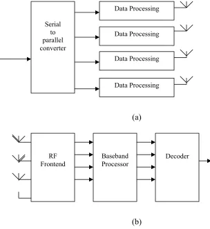
Figure 2.1: A MIMO system. (a) MIMO Transmitter. (b) MIMO receiver
Figure 2.1 shows a schematic representation of this multiple input multiple output
(MIMO) system [Adjoudani 2003]. The complexity of the MIMO systems is involved in
designing an optimal receiver for the system. The optimal receiver is a maximum-likelihood
sequence detector and is computationally complex due to system parameters like number of
antennas and type of constellation used. Therefore the optimal detection strategy is to equivalent
to performing a maximum-likelihood search over all possible transmitted symbol vectors. When
there is a perfect knowledge of channel state information at the receiver the sphere decoding
algorithm is considered as the maximum likelihood decoder.
There are two typical lattice decoding algorithms. One is the Pohst strategy based
algorithm [Viterbo 1999]. This tries to find lattice points inside a sphere of given radius. Another
is the Schnorr-Euchner strategy based algorithm [Eriksson 2002]. This method divides the lattice
into hyper-planes and starts the search for the closet point in the nearest hyper-plane.
2.2 Field Programmable Gate Array (FPGA)
FPGA is an integrated circuit that contains configurable (programmable) logic blocks and
interconnects between these blocks. In other words, it is a general purpose chip which can be
reconfigured any number of times to carry out specific hardware functions. It provides an
opportunity of instantaneous changes in designing and debugging. It allows for system reuse,
parallel design and SOC design. This is the result of combinatorial features of PLD and ASIC.
PLD is a digital IC that can be programmed by the user to perform a wide variety of logical
operations. ASIC is an IC product customized to perform specific functions to a particular
system or application. Like PLD, FPGA is completely prefabricated and contain special features
FPGA can be migrated to ASICs. A comparison between ASIC, FPGA, and DSP
implementations of the any decoder shows that the performance of FPGA-based designs lean
more toward that of ASICs but retain flexibility more like DSP [Gregory 1999]. ASICs provide
the most optimized hardware implementation of an algorithm. Using a dedicated ASIC for each
mode of radio leads to a very large silicon area. DSPs have excellent programmability but cannot
handle the complex algorithms at the required speeds with reasonable power consumption.
FPGAs on the other hand use hardware reconfiguration, which allows implementation of
complex high-speed algorithms [Srikanteswara 2003]. Compared to FPGA implementation, DSP
implementations require low cost and less development time. But once an efficient architecture is
developed and the parallelism of the algorithm is explored, FPGAs can be used to significantly
improve the speed of the signal processing or wireless communication systems. Thus, FPGA is
considered as an ideal platform for performing the computationally complex operations for
reasons of performance, power consumption and configurability. Compared to DSP chip,
parallelism is an additional feature in FPGA. The architecture of the Xilinx Virtex-II FPGA is
shown in Figure 2.2. The device is organized as an array of logic elements and programmable
routing resources used to provide the connectivity between the logic elements, FPGA I/O pins
and other resources such as on-chip memory, delay lock loops and embedded hardware
Figure 2.2: Virtex-II FPGA architecture [Chris]
The FPGA resources of particular interest to the signal processing engineer are
configurable dual-port block memories, distributed memory, and the multiplier array [Xilinx
2003]. The multiplier array is composed of 18x18-bit precision multipliers for addressing
advanced sign al processing applications. The smallest Virtex-II device provides a modest 4
3 Sphere Decoding Algorithm
This chapter describes the Pohst’s lattice point enumeration algorithm [Viterbo 1999]
widely known as sphere decoding, and also called universal lattice decoding. The data flow path
and state transition details are elaborated. High level description of the algorithm and decoder
architecture scheduling are also elucidated. The FSM diagram is shown. The table showing the
processing time taken by each state is presented.
3.1 The Sphere Decoder
In digital communications, lattice codes generate signal constellations for high rate
transmission. The high-rate data streams and spatial multiplexing leave MIMO technology as the
most desirable option in communication systems. The complexity of MIMO systems is involved
in designing a MIMO receiver. For designing a MIMO receiver, a ML decoding is employed.
ML decoding of a arbitrary lattice code used over an additive white Gaussian noise (AWGN)
channel is equivalent to finding the closest lattice point to the received point. To reduce the
complexity of an exhaustive search procedure, the bounded distance search among the lattice
points is formulated. Therefore, for decoding the optimal receiver output of these MIMO
systems, Pohst’s enumeration based sphere decoding algorithm searches for the closest lattice
point to the received point within the sphere with radius C. The center point i.e., the signal or
vector at the receiver is known before hand. The choice of C is very crucial to the speed of the
algorithm. In practice the choice of C can be adjusted according to the noise variance so that the
probability of a decoding failure reported is negligible. The complexity of the algorithm is
independent of the lattice dimension size, which is very useful for high data rate transmission
sphere with a certain radius in [Pohst 1985]. Then it was introduced into the field of digital
communications for the first time in [Viterbo 1993] and further analyzed in [Viterbo 1999].
3.1.1 Maximum-Likelihood Criterion
Considering a MIMO system with m transmit and n receive antennas, and a perfect
knowledge of channel state information is known at the receiver then the maximum likelihood
decoding requires minimization of metric
∑
= − n i i i x r 1 2 |||| ∀valid lattice points. Equation (3-1)
Where,r =uM +V , the received vector. When the data streams interfere with each other in the
channel and is distorted by an AWGN component V then, the resultant is the received vector.
u is the transmitted signal.
M is the channel matrix which generates the lattice.
V is the AWGN noise vector with zero mean and N0variance.
x is the information symbol vector mapped into the output vector which is the received vector r.
Thus x is considered as one of the transmitted lattice code points.
The representation of lattice points is given as {x=uM}where }u ={u1,u2,....un is the integer
component vector, and M is the channel transfer matrix which generates the lattice Λstructure.
Any lattice Λis given as the combination of set of basis vectors represented by v={v1,v2....vn}
Ifvi =(vi1,vi2....vib), i = 1………n, and b is the dimension of the lattice then the generator
matrix M of the lattice Λis defined as
The same lattice structure Λcan have any number of generator matrices. For example the matrix
of the formM' =TM , where T is an integer orthogonal matrix(det(T)=±1), is also the
generator matrix of the latticeΛ . Assuming matrix M to be non-singular square matrix
i.e.,n=b, the Gram matrix of the lattice Λis given by
= = bb b b T g g g g MM G L M M L 1 1 11
The elements of the matrix G are the Euclidean square products of the pairs of vectors of the
lattice basis.
3.1.2 ML Decoding In Sphere Decoder
The lattice decoding algorithm attempts to minimize the metric in Equation (3-1) but
employs the bounded distance search procedure. Thus it searches through the points of lattice
that are falling inside the sphere of radius C and centre at the received point.
Thus, sphere decoding problem is to solve
|| || min || ||
min r x w
r w
x∈∆ − = ∈−∆ Equation (3-2)
So we search for the shortest vector w in the translated lattice r−Λ in the n-dimensional
Euclidean spaceRn. We write
uM
x= with u∈zn
M
r= ρ with ρ =(ρ1,ρ2...ρn) ∈Rn
∑
= = = n i i iv M w 1 ξξ with ξ =(ξ1,ξ2....ξn) ∈Rnand ξi =ρi −ui,i=1,....n
1
− =rM
ρ i.e.,ρis equal to the matrix product of the received vector ,r and the inverse of
generator matrix M−1. ξ defines the translated coordinated axes in sphere of the integer
component vectors uof the cubic latticeZn
3.2 Flow-Chart
The flow chart showing of a Lattice decoding algorithm [Viterbo 1999] or a Universal
lattice decoder is shown in Figure 3.1. The lattice decoding algorithm can be divided into two
parts (1) Pre-processing part (2) Decoding part.
3.2.1 Pre-Processing
The pre-processing stage of the sphere decoding algorithm involves the complex
computations like Cholesky decomposition of the Gram matrix G, finding inverse and transpose
of generator matrix M. The resultant matrices are passed to the decoding part where they are
further exploited to carry on other computations, thereby reducing the complexity of the
decoding part. The variables and specialized functions used at this stage are described in detail
below.
An inverse matrix of the lattice generator matrix is computed. Another important function
carried out in the preprocessing stage in the algorithm is the Cholesky factorization of the Gram
matrixG. Gram matrix is equal to the product of lattice generator matrix M and its transpose,
T
MM
G= yieldsG= RTR where, R is the upper triangular matrix.
From the algorithm (qj,k) is the element of Cholesky factor matrix.
3.2.2 Decoding
In the decoding part, the integer component of lattice point vector u closest to the
transmitted signal constellation x is found as an output when the Cholesky factor matrix(qj,k) ,
the square radius of the sphere C and the received vector with respect to lattice ρ are taken as
inputs.
Considering the metric properties of the lattice, we can say that the minimum squared
Euclidean distance between any two points of lattice equals the minimum of the quadratic
formQ(ξ).
T T
T MM
G
If the lattice point being searched is within the sphere with square radius C and centered at the
received point then
∑∑
= = ≤ = = = n i n j j i ij TT g C
MM Q w 1 1 2 )
(ξ ξ ξ ξξ Equation (3-3)
Thus the sphere of square radius C and centered at the received point is transformed into an
ellipsoid centered at origin of the new coordinate system defined byξ.
Cholesky factorization yieldsG=RTR, where R is an upper triangular matrix. By further
analyzing the above equations we get
∑
∑
= =+ ≤ + = = = n i n i j j ij i ii TTR R r r C
R Q 1 2 1 2 ) ( )
(ξ ξ ξ ξ ξ ξ Equation (3-4)
Substituting qii =rii2and qij =rij/rii for i = 1,…, n, j = i + 1,…, n, we can write (3-4) as follows
∑
∑
= =+ ≤ + = n i n i j ij j iii q C
q Q 1 2 1 ) ( )
(ξ ξ ξ Equation (3-5)
We find the equations of the border of the ellipsoid to estimate the upper and lower
bounds of the integer component value ui at the ith layer. Therefore the ranges for the integer
component value at ithlayer are given by
Equation (3-6)
Thus the upper bound,Li and the index, uiare simplified as follows
Equation (3-7) Equation (3-8) + + + − ≤ ≤ + + + − −
∑
∑
∑
∑
∑
∑
+ = + = =+ + = + = =+ n i j j ij i n i l n l j j lj l ll ii i n i j j ij i n i l n l j j lj l ll ii q q q C q u q q q C q 1 1 1 2 1 1 2 1 ) ( 1 ) ( 1 ξ ρ ξ ξ ξ ρ ξ ξ
/
1Where, the variables Si and Ti are written as l il n i l i n l i i q
S ξ ξ ρ ξ
1 ) ... ( + =
+ = + Σ Equation (3-9)
− = = −
− T C
Ti 1 i1(ξi...ξn) n lj j l
j=Σ+1q ξ =
2
) ( i i ii
i q S u
T − − Equation (3-10)
Thus the variablesSi, Ti and one of the outputs of the pre-processing part qii are used to
determine and recursively update the values of bounds.
The index uiis initially fixed at the lower bound and incremented in steps until it exceeds
the upper bound of that layer. Search procedure starts at the bottom layer i.e., at i=4and
continues switching the layers step by step by checking various conditions at each layer until it
reaches the top layer and a valid lattice point vector is reported. When the vector inside the
sphere is found, its square distance from the center is computed which is given by
2 1 1 11 1
2 C T q (S u )
dΛ = − + − Equation (3-11)
This value is compared to the minimum square distance d2(initially set equal to C) found
so far in the search. If it is smaller then we have a new candidate closest point and new value
ford2 updated with dΛ2 . Thus the search continues like this until all the vectors inside the
sphere are tested.
If no point in the sphere is found the sphere is declared empty and the search fails. In this
case the squared radius C must be increased and the search is restarted. Thus finally we search
the lattice point closest to received point.
The advantage of this method is that we never test the vectors which are present outside
3.3 Decoding Procedure
The original sphere decoding algorithm performs step-by-step procedure as follows,
The inputs are C,ρ,Q and output is uΛ
Step 1. (Initialization)
Set i=n,Tn =C,d2 =C(current sphere square radius) and
Step 2. (Bounds on index ui)
Compute the upper and lower bounds. Assign the upper bound toLi and the lower bound
to index uiinitially. Thus
Step 3. (Natural spanning of the interval)
Increment the index uiby one step, i.e.,ui =ui +1
If ui ≤Liandi>1, i.e., the index is within the range and layer is not the top layer then go to Step
5, else if ui ≤Liandi=1, i.e., the index of the top layer is within the bound then go to Step 6,
else if ui >Li go to Step 4.
Step 4. (Increase i: move one level down)
If i=nterminate, i.e., the end of the search procedure is reached and closest lattice point
to received point is found, else set i=i+1, i.e., the search procedure goes one level down in the
hierarchy, and go to Step 3.
Step 5. (Decrease i: move one level up)
n k
Sk =ρk, =1...
/
1/
− + −
=
+ =
i ii i i
i ii i i
S q T u
Let ξi =ρi −ui
l l i n
i l i
i q
S 1 ρ 1 −1,ξ = −
− = +Σ
2
1 i ii( i i)
i T q S u
T− = − −
1
− =i
i and go to Step 2.
The variables needed to recursively update the lower and upper bounds are computed at this step
and the search procedure goes one layer up in the hierarchy to re-compute the upper bound and
indexui.
Step 6. (A valid point is found)
Compute 2
1 1 11 1
2 C T q (S u )
dΛ = − + − , the square distance of the vector found from the
center. Then compare this value to the minimum square distance d2 i.e., If dΛ2 <d2 then save
the lattice point, uk =uk,k =1....n Λ
and reduce the search area by assigning the minimum square
distance value d2with dΛ2 and the variable
n
T at the bottom layer with dΛ2 and again set i=n.
Then go to Step 2 repeat the whole process once again. Else go to Step 3, where the index value
i
u at each layer is incremented and the search procedure continues as mentioned.
3.4 High Level Simulation of the Sphere Decoding Algorithm
Before actually carrying out the implementation of the sphere decoding algorithm in the
next section, which is the main concern of our thesis, it was felt necessary to visualize the
functionality and working of the sphere decoder. Therefore the whole algorithm, including both
2 2
2 =dΛ ,T =dΛ
pre-processing and decoding parts is initially developed in Matlab for simulating at behavioral
level. The complete system is brief below:
• Generation of Lattice generator matrix based on normally distributed random numbers
generated using MATLAB function “randn”
• Generating the upper triangular matrix by Cholesky decomposing of the gram matrix.
• After the input information to the decoder is ready, sphere decoding algorithm which finds
the closest lattice point is simulated using Matlab. Its functionality is verified by comparing the
obtained lattice point with the transmitted signal constellation vector.
The functionality of the decoder is verified at high level of abstraction and behavior of
the decoder design is simulated using Matlab. Thus preliminary information of outputs is
obtained. After ensuring the functionality of the decoder design, the corresponding hardware
architecture is planned.
3.5 Decoder Architecture Scheduling
The hardware architectural model of Sphere decoder is planned in accordance with the
simulated version. Each of the operations like calculating the bounds, calculating variables
needed to update the bounds, spanning of index at each level and finding the Euclidean distance
of a point from the received point are dealt in separate blocks. Different components are
designed for specific set of operations at each block. Each of these blocks are designed in VHDL
and tested for their functioning with the help of stand alone test benches and different sets of
data. Digital circuit designs are invariable faced with the need to design circuits that perform
specific sequence of operations, for example controllers used to control the operation of other
circuits [Smith 1997]. Thus the decoder controller is designed for the hardware architecture of
algorithm divided into states is shown in Figure 3.2. FSMs are proven to be a very efficient
means of modeling sequencer circuits. By modeling FSMs in a HDL for use with synthesis tools,
focus could be on modeling the desired sequences of operations without being overly concerned
with circuit implementation. In Figure 3.4 the state diagram of the decoder controller is given.
Sequences of operations which are almost independent of each other are combined into one
single state. While state division, care is taken in regard of processing time needed at each state
to maintain balance at the end of simulation of the algorithm.
Here, in our case, the six steps of the sphere decoder are modeled to four states FSM.
This is because sequence of operations at some steps which do not really need separate states are
combined with others and modeled into a single state. The Step 1, Step 2 and Step 3 are
combined and modeled as State A. Step 5 as State B. Step 3 is combined with Step 4 and
modeled into State C. Step 6 as State D. Since Step 3 involves simple index increment it need not
be a separate state. It could be a part of State A or State C based on the requirement. If index has
to be incremented immediately after it is assigned with lower bound, then it is part of State A. If
3.5.1 Data Flow of the Algorithm
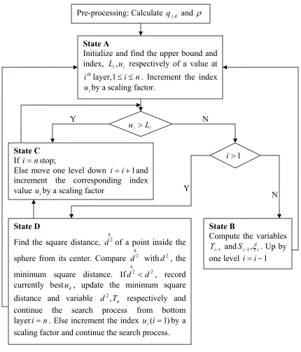
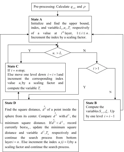
Figure 3.2: Flowchart of a Sphere decoding algorithm showing states
As seen in Figure 3.2, the computations at each of the four states in the recursive lattice
decoding algorithm are discussed in detail here. Along with the states and state transitions, the Pre-processing: Calculate qj,k and ρ
State A
Initialize and find the upper bound and index, Li,ui respectively of a value at
th
i layer,1≤i≤n. Increment the index
i
u by a scaling factor.
i i L
u >
State C If i=nstop;
Else move one level down i=i+1and increment the corresponding index value uiby a scaling factor
1
> i
State D
Find the square distance, dΛ2 of a point inside the
sphere from its center. Compare dΛ2 withd2, the
minimum square distance. IfdΛ2 <d2, record
currently bestuk, update the minimum square distance and variable d2,Tn respectively and
continue the search process from bottom layeri=n. Else increment the index ui(i=1)by a scaling factor and continue the search process.
State B
Compute the variables
1
− i
T andSi−1,ξi. Up by one level i=i−1
Y N
Y
components enabled at each state are also discussed in detail. As we said earlier the
computations are divided into four components.
In State A, it finds the upper and lower bounds of an integer component value at each
layer. The variable Liis assigned an upper bound and the index ui is initially set at lower bound.
Separate hardware component is designed for computing the square root. The decoder controller
when in State A, enables the all the functional blocks designed to compute the above variables.
In State B, it computes the variablesTi, and move one layer up. These variables are Si
used to recursively update the lower and upper bounds at that layer. A functional block to
compute the above variables in enabled at this state by the decoder controller. In addition to that
the functional blocks active in previous state are disabled by the decoder controller.
In State C, check the layer at which search procedure is currently present. If it is the
bottom most layer, terminate the search procedure and declare the last saved u as the closest
lattice point. If the search procedure is at layers other than the bottom most layer move one layer
down and increment the index value uiat that layer by the scaling factor. At this state, the
spanning of the interval at each layer, i.e., incrementing ui is performed by the enabled
functional block. All other details are taken care by the decoder controller.
In State D, thedΛ2 , the square distance of uΛthe lattice point present inside the sphere from
center of the sphere or the received point is computed and is compared with the minimum square
distance d2. Based on this, decision about the next state is made by the decoder controller.
At each state after obtaining the output from the blocks the decoder controller makes the decision
about the next state in the current state. Decoder controller is designed in such a way that it
blocks of current state in the first clock cycle of current state itself. Thus when all the required
conditions are met and all the sequence of operations are completed the results are output. The
functioning of the decoder controller and all its components is tested using a test bench.
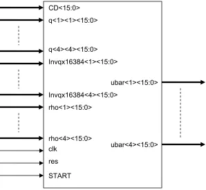
The pin diagram of the decoder controller for the original sphere decoding algorithm and
its functionality is shown in is shown in Figure 3.3 and Table 3.1.
Figure 3.3: Input and Output pins for original sphere decoder CD<15:0>
q<1><1><15:0>
q<4><4><15:0> Invqx16384<1><15:0>
ubar<1><15:0>
ubar<4><15:0> Invqx16384<4><15:0>
rho<1><15:0>
rho<4><15:0> clk
res
Table 3.1: Pin descriptions for the decoder controller of the original sphere decoding algorithm
Pin Width Type Description
CD 16 Input square radius of the sphere
q(1,1) - q(4,4) 16 Input elements of Cholesky factor matrix
Invqx16384(1) –
invqx16384(4 16 Input Inverse of diagonal elements of the Cholesky factor matrix
rho(1) - rho(4) 16 Input coordinates of received point vector with respect to lattice
clk) 1 Input clock signal
res 1 Input reset signal
START 1 Input control signal to initialize the current state
ubar(1) - ubar(4) 16 Output coordinates of the closest lattice point being searched
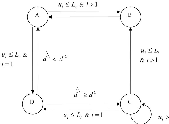
3.5.2 FSM Design
A finite state machine (FSM) of a decoder controller is designed to control and organize
the sphere decoding algorithm and it synchronizes the operations between functional blocks. The
five parametersui,Li, the index and upper bound respectively at the current investigated layer of
the lattice, the layer i(1≤i≤n),the square distance of the lattice vector inside the sphere from
the received vector dΛ2and the minimum square distance d2determine the state transitions as
shown in the Figure 3.4 below.
If the search procedure is in State A then after computing the index uiand upper
boundLi, it checks for the conditions if the index is within range of the upper bound or equal to
upper bound and the current layer is not the top layer then the control goes to State B. At State B,
after State B control goes back to State A and continues to carry out the operations at this state.
Again when in State A, it looks for the condition if the index is within the range of upper bound
or equal to it and the current layer is the top layer then control moves to State D from State A.
And if index exceeds the upper bound at any layer then the control moves to State C from State
A. When the decoder controller is in State D, it computes square distance dΛ2 and compares it
with the minimum square distanced2, if it is less then control goes to State A from State D and
whole search procedure repeats once again. And if dΛ2is greater than or equal to the value of
2
d then controller moves from State D to State C. At State C the index value is incremented and
the conditions are checked. The state transition from State C to other states is same as it was
from State A to other states.
Figure 3.4: The FSM diagram of Sphere decoding algorithm
A B
C i
i L
u ≤ & i>1
D i i L
u ≤ &
1
= i
i i L
u ≤ & i>1
i i L
u >
Λ
2
d ≥d2
Λ
2
d < d 2
i i L
3.6 Simulation Results
The decoder core is designed in VHDL at register transfer level (RTL). Mentor Graphics’
Modelsim SE 5.8 tool is used to create, compile and simulate the VHDL source code of the
decoder core. A design library named work is automatically created in the project directory upon
creating the new project and all the necessary design files and test bench are held together in the
project directory. The VHDL source code is compiled to test its syntax. Successfully compiled
source code is simulated using different sets of data. At the simulation step, initially the design is
loaded successfully if no errors are reported. View the signals of the design and add the
necessary signals to the waveform window. Run the wave until output results of the whole
design are obtained. Processing time taken by each state of the decoder controller individually
can be acquired from the wave. Table 3.1 shows the processing time of each state of FSM of the
Sphere decoder after successful VHDL simulation.
Table 3.1: Simulation Times of each state in original algorithm
State A B C D
Simulation Time in
clock cycles 37 7 2 7
The determination of lower and upper bounds of an integer component value at a
particular layer involves a 32-bit square root computation. To compute the square-root, here we
made use of non-restoring algorithm explained in Section 3.6.1
3.6.1 Non-Restoring Square Root Algorithm
In this algorithm [Piromsopa 2001], the radicand is a 32-bit unsigned number. The square
Since this is a redundant representation for a square root, exact bit can be obtained in
each iteration.
Let
D be 32-bit unsigned integer.
Q be 16-bit unsigned integer (Result) R be 17-bit integer (R=D−Q2) Algorithm ; 0 ; 0 = = R Q
For i = 15 to 0 do If (R≥0)
); 1 ) (( ); 3 ) ( ( ) 2 ( or Q R R and i i D or R R << − = + >> << = Else ); 3 ) (( ); 3 ) ( ( ) 2 ( or Q R R and i i D or R R << − = + >> << =
End if
If (R≥0) then
; 1 ) 1 (Q or Q= <<
Else
; 0 ) 1 (Q or Q= <<
End if
The above non-restoring algorithm for calculating the square-root of a number is
explained clearly by considering an example. Here in the example we consider D as an 8-bit
radicand equal to value 140(100011002). The 4-bit solution Q should be 11(10112) and
remainder R should be equal to 19(100112).
1011 Q 0, R 010011 010101 -101000 R 0, R 0, i 0101 Q 0, R 001010 001011 011111 R 0, R 1, i 0010 Q 0, R 011111 000101 000100 R 0, R 2, i 0001 Q 0, R 000001 000001 000010 R 0, R 3, i = ≥ = = ≥ = = ≥ = + = < = = < = − = ≥ = = ≥ = − = ≥ =
To correctly determine value of R, one more extra bit is added (Consider as sign bit).
Thus the result Q is obtained.
From the simulation results of the sphere decoder core it is seen that sequence of
operations at State A take 37 clock cycles. Out of this, 32 clock cycles are needed for a square
root computation. The sequences of operations at other states take less than 10 clock cycles.
Comparing with the other states, processing time of State A is remarkably high. Due to this
imbalance and very high processing time, the throughput of the system is affected noticeably.
This imbalance has to be removed for efficient and high throughput implementations. This
eventually results in an un-efficient hardware implementation of the sphere decoding algorithm.
An improved form of the algorithm is suggested with modifications in the sequences of
operations of each functional block. These modifications are such that the square root
4 Improved Sphere Decoding Algorithm
The improved sphere decoding algorithm is derived with modifications applied to the
sequences of operations at each state of the original algorithm in this chapter. The dataflow of
the improved algorithm is discussed. A table showing hardware processing time needed by each
state is given. Data dependency of the algorithm is also analyzed.
4.1 Improved Sphere Decoding Algorithm
An improved sphere decoding algorithm is proposed. The need for the improved
algorithm arises from the simulation results of the original algorithm. As we have seen, State A
of the original algorithm requires 37 clock cycles for completion, out of which 32 clock cycles
are taken by square root itself. On the other hand the processing time required by each of the
remaining states is limited to very few clock cycles (Refer Table 3.1). The sequences of
operations at other states have to wait for the completion of State A if they are depending on the
results of State A. This time delay can be reduced if the square root computation is avoided.
Therefore we suggest some modifications to the original algorithm such that square root is
avoided in its sequences of operations and as a result emerges an improved sphere decoding
algorithm. The derivation of modifications is given in Section 4.1.1. The sequence of operations
at State A of the improved algorithm use simple adders and multipliers to compute the upper
bound Li and the index ui. Since there is no square root computation involved, a hardware
component to compute square root is no longer needed. In the improved algorithm, modifications
are present at the sequences of operations, whereas the state division and the state transition
decisions depending on the outputs obtained from the functional blocks at each state remains the
4.1.1 Derivation of Modifications
As we know the minimum squared Euclidean distance between any two points of the
lattice equals the minimum of quadratic from Q(x) for any x∈Zn[Viterbo 1993]. Applying this
to the sphere decoder, squared Euclidean distance between any point inside the sphere and
received point must be less than or equal to the square radius of the sphere.
C Q
w2 = (ξ)≤ Equation (4-1)
∑
∑
= =+ ≤ + n i n i j j ij iii q C
q
1 1
2 )
(ξ ξ Equation (4-2)
Expanding this, we get
... ) ... ( ) ... ( 2 2 3 23 2 22 2 1 2 12 1
11 +q + qn n +q +q + q n n +
q ξ ξ ξ ξ ξ ξ +
qn− n− n− +qn− n n 2 +qnn n2 ≤C ) 1 ( 1 ) 1 )( 1
( (ξ ξ ) ξ Equation (4-3)
We know that ξi =ρi −ui Equation (4-4)
Substituting equation (4-4) in (4-3), we get
+ + − + − + − + − + + − + − ( ) ... ( )) ( ( ) ( )) ... ( 2 4 4 24 3 3 23 2 2 22 2 1 2 2 12 1 1
11 u q u q u q u q u q u
q ρ ρ n ρn n ρ ρ ρ
C u
qnn(ρn − n)2 ≤ Equation (4-5)
Equation (4-5) cannot be solved because of presence of n unknowns. Therefore we need to split
the expression and solve it. Due to the upper triangular form of Cholesky factor matrix, equation
(4-5) represents a set of conditions.
at i = n, qnn(ρn −un)2 ≤C Equation (4-6)
at i = n-1, qn− n− n− −un− +qn− n n 2 +qnn n 2 ≤C
, 1 1 1 1 ,
1 (ρ ξ ) (ξ ) Equation (4-7)
Equation (4-6) can be solved easily because of only one unknown i.e.,un. Considering the above
conditions in the order from n to 1 i.e., starting at the bottom layer and carrying on the backward
substitution, we obtain the admissible values of each symbol uifor known values ofui+1,K,un.
The range of the index ui as found in the original algorithm is given as
Equation (4-8)
In equation (4-8), the upper and lower bounds of index ui are found by using a square root
computation. The main idea in the improved algorithm is to avoid square root
At ith layer, equation (4-5) can be written as
+ + − + − + − + + − + − + ( + + ) ... ( )) + + ( + + + + ( + + ) ...
( 2 1, 1 1 1 1, 2 2 2
1 1 1
,i i i in n n i i i i i i i i
i i i
ii u q u q u q u q u
q ρ ρ ρ ρ ρ
C u
qnn(ρn − n)2 ≤ Equation (4-9)
Simplifying it further,
C q u q q u q n i l n l
j lj j
l l ll n
i
j ij j
i i
ii − +
∑
+∑
− +∑
≤+ = =+ + = 1 2 1 2 1 ) ( )
(ρ ξ ρ ξ Equation (4-10)
When the search procedure completes, index vector u should be the closest point to the
transmitted signal. Because signal constellation is known at the receiver part, a new method of
determining the search range of lattice index can be achieved by directly substituting each
symbol from the signal constellation into equation (4-10). Here we assume the integer
component value uias one among the signal constellation elementsxk,k =1....n (For a 4-PAM
signal, symbol set is ranging as {-3, -1, 1, 3}) then equation (4-10) can be written as
C q u q q x q n i l n l j j lj l l ll n i j j ij k i
ii − +
∑
+∑
− +∑
≤+ = =+ + = 1 2 1 2 1 ) ( )
(ρ ξ ρ ξ Equation (4-11)
If we redefine variable Tl as
( )2
l l ll
l q S u
T = − Equation (4-12)
and variable Siholds the same definition as in the original algorithm described in equation (3-9)
∑
+ = + = n i j j ij i i q S 1 ξρ Equation (4-13)
Finally by substituting equation (4-12), (4-13) in equation (4-11), we get the expression
C T x S q n i l l k i
ii − +
∑
≤+ = 1 2
)
( Equation (4-14)
∴ p q S x n T C
i l l k i ii
k = − +
∑
≤+ = 1 2
)
( ∀values of k =1....n Equation (4-15)
The upper bound, Li =max(xk)∀ pk ≤C
The index, ui =xr −1for pr =min(pk)≤C ∀values of k =1....n
If vector p is empty, then the upper bound Liand index uiare assigned with maximum
and minimum values of signal constellation.
Considering an example to explain this in detail, at SNR = 20 dB and generator matrix M
is given as
− − − − − = 6686 . 0 6900 . 0 5937 . 1 6236 . 1 2902 . 1 3999 . 0 2540 . 1 7143 . 0 7119 . 0 5711 . 0 8580 . 0 3362 . 1 8156 . 0 4410 . 0 6918 . 0 2944 . 0 M
Then the received signal obtained after scaling and rounding is equal to
to
[
384 128 −128 −384]
. Assuming the appropriate choice of squared sphere radius, C = 512 (after scaling and rounding). In such a case, the sequence of operations to find the indexui, andupper bound Li go as follows.
at i = 4, p = [2714 1193 289 0]
The upper bound, Li =max(xk) = max (-128, -384) = -128
The index, ui =xr −1for pr =min(pk)≤C
0
= r p
512 − = ∴ui
This avoids square root computation while finding upper and lower bounds. And thus the
index ui takes the value within the range of signal constellation. The main advantage achieved
from this improved sphere decoding algorithm is the significant reduction in the processing time
of State A when the algorithm is prototyped on hardware. The flowchart of the improved
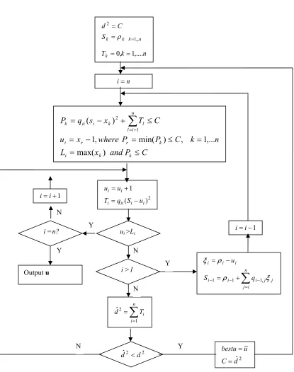
4.1.2 Flow-Chart
Figure 4.1: Flow chart of improved algorithm
Y n k T S C d k n k k k ,.... 1 , 0 ,, 1 2 = = = = = ρ n i= C P and x L n k C P P where x u C T x s q P k k i k r r i n i l l k i ii k ≤ = = ≤ = − = ≤ + − =
∑
+ = ) max( ,... 1 , ) min( , 1 ) ( 1 2 2 ) ( 1 i i ii i i i u S q T u u − = + =∑
= = n i i T d 1 2 ˆ∑
= − − − = + − = n i j j j i i i i i i q S u ξ ρ ρ ξ , 1 1 1 1 − =i i 1 + =i iui >Li
i >1
2 2
ˆ d
d < ˆ2
4.2 Decoding Procedure
The original sphere decoding algorithm performs step-by-step procedure as follows,
The inputs are C,ρ,x,Q and output is uΛ
Step 1. (Initialization)
Set i=n,Tk =0,d2 =C(current sphere square radius) and
Step 2. (Bounds on index ui)
Compute the parameter pk such that the upper bound and index values are found.
ThusP q s x n T C i
j l k
i ii
k = − +
∑
≤+ = 1 2 )
( ,(k =1,...n)
where x
Li =max( k), Pk ≤C
, ) min( ,
1where P P C
x
ui = r − r = k ≤ (k =1,...n)
Here when signal constellation vector is known, the upper bound and index can be computed.
Step 3. (Natural spanning of the interval)
Increment the index uiby one step, i.e.,ui =ui +1and compute the variable Tiat each
layer i. Thus ( )2
i i ii
i q S u
T = −
If ui ≤Liandi>1, i.e., the index is within the range and layer is not the top layer then go to Step
5, else if ui ≤Liandi=1, i.e., the index of the top layer is within the bound then go to Step 6,
else if ui >Li go to Step 4.
n k
![Figure 2.2: Virtex-II FPGA architecture [Chris]](https://thumb-us.123doks.com/thumbv2/123dok_us/8939301.1849069/19.612.156.438.95.323/figure-virtex-fpga-architecture-chris.webp)
![Figure 3.1: Flowchart of a Sphere decoding algorithm [Viterbo 1999]](https://thumb-us.123doks.com/thumbv2/123dok_us/8939301.1849069/23.612.104.483.286.687/figure-flowchart-sphere-decoding-algorithm-viterbo.webp)