A Simulation of the Quenching Process for Predicting Temperature, Microstructure and Residual Stresses

A Simulation of the Quenching Process for Predicting

Temperature, Microstructure and Residual Stresses

Caner Şimşir1 _{- C. Hakan Gür}2,*

1 _{Stiftung Institüt für Werkstofftechnik, Germany}

2 _{Middle East Technical University, Metallurgical and Materials Engineering Department, Turkey}

A finite element model capable of predicting the temperature history, evolution of microstructure and residual stresses in the quenching process is presented. Proposed model was integrated into Msc. Marc® software via user subroutines. Verification of the model was performed by X-ray diffraction residual stress measurements on a series of steel cylinders quenched.

©2010 Journal of Mechanical Engineering. All rights reserved.

Keywords: steel quenching, simulation, finite element method, microstructure, residual stress

0 INTRODUCTION

Quenching of steels is a multi-physics process involving a complicated pattern of couplings among heat transfer, phase transformations and stress evolution. Physical fields interact with each other either by sharing of state variables or coupling interactions. Because of the complexity, coupled (thermal-mechanical-metallurgical) theory and non-linear nature of the problem, no analytical solution exists; however, numerical solution is possible by the finite difference method, finite volume method, and the most popular one - finite element method (FEM). Heat transfer to the quenching medium is the driving physical event as it triggers other processes, and thus, quenching techniques are usually nominated as immersion quenching, spray quenching or gas quenching. Variation of temperature at any point in the component is the major driving force for phase transformations. Upon cooling, thermodynamic stability of parent phase is altered, which results in decomposition of austenite into transformation products. The transformation rate depends on the temperature and the cooling rate. On the other hand, there is a heat interaction with the surroundings during phase transformations. Phase transformations that occur during quenching are exothermic and they alter the thermal field by releasing latent heat of transformation.

Thermal stresses are generated in the quenched component due to large temperature gradients and the variation of mechanical properties with temperature. Varying cooling rates at different points lead to varying thermal contractions which must be balanced by an

internal stress state. Those stresses may cause a non-uniform plastic flow when their magnitude at any point exceeds local yield strength. On the other hand, since plastic deformations are relatively small (< 3%) in the quenched part, heat induced by plastic deformation is neglected.

During decomposition of austenite into transformation products such as ferrite, pearlite, bainite and martensite, a volume increase is observed in the transforming region due to density difference between the parent and the product phases. Those strains are the primary source of fluctuating internal stress field, besides the thermal stresses and transformation induced plasticity (TRIP). It refers to the irreversible strains produced by the interaction of macroscopic stress and the microscopic plasticity due to phase transformations.

In addition, stress and plasticity affect the phase transformations by altering both the thermodynamics and the kinetics of the transformation. Most commonly observed effect of stress on transformation diagrams is the shift of critical temperatures and times. In some cases, transformations may be induced or totally inhibited by stress. This concept is generally referred to as stress induced/inhibited phase transformation.

temperature at any point in the part, a non-uniform plastic flow occurs.

A lot of research has been conducted to develop numerical simulation tools for prediction of final state of the component after quenching.

The first studies on prediction of microstructure and residual stress distribution in quenching by computer simulation originate from the early 1970s. In the early 1980s, many studies for the implementation of phase transformation effects in the previously developed models were conducted. In the second half of the 1980s, many research groups developed improved constitutive models for material behavior during quenching of steels. The first mature models for the effect of stress on phase transformation and TRIP were developed. Previously neglected physical phenomena such as plastic memory loss during phase transformations, effect of stresses on the transformation thermodynamics and kinetics, transformation plasticity were implemented in the simulations. The theory of heat transfer during quenching, the selection of quenchant, and fundamentals of intensive quenching were presented. In 1990s, improvements in computational power and the finite element software lead to an acceleration in research; especially the concepts of calculation TTT and CCT diagrams and TRIP became more mature. Several commercial FEA software simulating quench processes became available. Since 2000, from the viewpoint of development of new technologies to control quenching, many articles and reviews have been published. Simulation of gas quenching and coupling quenching simulations with computational fluid dynamics (CFD) calculations have become a major interest. Currently, most of the research is focused on single phase gas quenching. Although CFD calculations still requires considerable amount of computational power, single phase calculations can be performed. These kind of simulations allow engineers to optimize of gas quenching system to minimize the distortion and to obtain optimum residual stress and microstructure distribution. However, the simulation of fluid flow during immersion quenching, which is the most common process in the industry, is not yet performed. The major drawback is quantitative description of thermo-physical events occurring on the surface during quenching. Extensive literature review about the simulation of

quenching and thermal treatments can be found elsewhere [1].

This paper presents a 3-D FEM based model of quenching, which is integrated into commercial software Msc.Marc via user subroutines to predict temperature history, evolution of microstructure and residual stresses.

1 MODELLING

1.1 Heat Transfer  

Quenching can be defined as a transient heat conduction problem with convective and radiation boundary conditions with internal heat source and sink. Basically, heat is removed from the surface of the specimen by convective heat transfer to the quenchant and by radiation, which results in thermal gradients driving the conduction inside the component. The essential point in modeling of quenching is the addition of an internal heat source term into this equation. The origin of this term is the latent heat released by phase transformations.

The transient heat transfer within the component during quenching can mathematically be described by an appropriate form of Fourier’s heat conduction Eq. (1). Considering that the thermal field is altered by the latent heat of phase transformations, the equation can be expressed in its most general form as,

( ). ( ). ( ( ). ) TR( , )

p T

T c T div T T Q T t

t

ρ ∂ = λ ∇ +

∂   (1)

where ρ(T), cp(T) and λ(T) is the density, specific heat, thermal conductivity of the phase mixture given as a function of temperature and QTR _{is the} latent heat release rate due to phase change. Thermal properties of the phase mixture is approximated by a linear rule of mixture,

1

( , ) .

N

k k k

P T ζ =

∑

where P represents a thermal property of the mixture. Pk and ζk are a thermal property and fraction of kth _{constituent, respectively.}

To incorporate the effect of latent heat, a fictitious specific heat (Cp*) is defined as,

( )

1 1 1

/

. .

/

N N N

k k

p p _k k k p k

k k k

d d dt

c c H c H

dT dT dt

ζ ζ

ζ

= = =

=

∑

∑

∑

Then, initial and boundary conditions are set to complete the thermal problem definition. Initially all nodal temperatures are set to austenitization temperature. The surfaces in contact with the quenchant have a film heat transfer boundary condition with surface temperature dependant heat transfer coefficient in the form of:

( ,T T_s ) h T T( )(_{s s} T )

ψ _∞ = − _∞   (4)

where Ts, T∞ , ψ and h are surface temperature,

quenchant temperature, heat flux and temperature dependant heat transfer coefficient, respectively. The use of a temperature dependent heat transfer coefficient allows simulation of different cooling regimes in different stages of quenching (vapor blanket, nucleate boiling, and convective cooling). Symmetry surfaces and surfaces which are not in contact with quenchant are assumed to be insulated surfaces by setting the heat flux to 0 as:

0

T n Ψ = −λ∂ =

∂   (5)

where n represents the unit normal vector.

1.2 Phase Transformations

Phase transformations can be categorized into diffusion controlled transformations and martensitic transformation, for which calculation of microstructural evolution requires different approaches. Since each point in the specimen has a distinct thermal history, the simulation of phase transformations requires mathematical models for anisothermal transformations. Different thermal paths will result in different amount of the product phase although all paths start and finish at the same temperature and time. Thus, both T and t can not be used as state variables. This realization introduces the notion of "additivity", which was first proposed by Scheil [2]. This concept was later extended to solid state phase transformation by Cahn [3], and generalized by Christian [4].

Additivity principle has long been discussed, reviewed and adopted by many authors [5] to [18]. General conclusion that can be drawn from these studies is that conventional Scheil-Cahn-Christian additivity principle is not quite accurate in the calculation of anisothermal kinetics from isothermal kinetic data. Some of the cited works improved the additivity principle to

achieve a better fit with experimental data, however; most of these methods require additional experiments to be performed.

The critical temperatures for phase transformations can directly be extracted from TTT and equilibrium phase diagrams or calculated using analytical expressions. In literature, there are several proposals: some of them are based on thermodynamic calculations, whereas the others are purely phenomenological expressions based on regression analysis. Kinetic parameters can be extracted from TTT and CCT diagrams or can be determined experimentally by measuring any property which is sensitive to phase transformations (such as volume, heat response, conductivity, magnetic permeability change etc.).

Diffusion Controlled Phase Transformations Diffusion controlled transformations occur by an incubation period followed by a transformation stage. In order to calculate incubation time required for a diffusional transformation under anisothermal conditions, isothermal transformation diagram (IT) data and Scheil`s additivity principle is used. According to Scheil`s additivity rule, if τ(ξk, T) is the isothermal time required to reach certain transformed amount ξk, the same transformation amount will be reached under anisothermal conditions when the following Scheil`s sum (S) equals to unity [2]:

1

1 ( , ) n

i

k i i

t S

T

τ ξ

=

Δ

=

∑

where Δti , τi are the time step size and isothermal time to reach ξk at the current time step.

Next, growth kinetics needs to be calculated. After the incubation period (S = 1), anisothermal growth kinetics is calculated using a modified Johnson-Mehl-Avrami-Kolmogorov (JMAK) Eq. (7) and Scheil`s additivity principle [19].

(

)

(

(

)

)

max 1 1 _{1 exp ( ).} n Tk

j j j

k k γ k b Tk j

ζ ₌ζ ζ − ₋ζ − _{− −} τ

(7) where ζkj , ζγj are the volume fractions of kth

microstructural constituent and austenite at current (jth_{) time step. ζ}

( )

(

)

1 ( )

ln 1 ( )

k

j n T

k j j k t b T ζ τ − ⎛_{− −} ⎞ ⎜ ⎟ = Δ + ⎜_⎜ ⎟_⎟ ⎝ ⎠   (8)

bk(T) and nk(T) in Eq. (7) are material constants that can be extracted from IT diagram by:

(

)

ln ln(1 ) / ln(1 )

( ) ln / s f k s f n T t t ζ ζ ⎡ − − ⎤ ⎣ ⎦

=   (9)

( )

ln(1 )

( ) k

k

k n T

k b T t ζ − − = ₍₁₀₎

where ζs, ζf are the fractions of transformed phase at the beginning and at the end of the growth stage, which are generally 0.05 and 0.95, respectively.

For proeutectoid ferrite tranformation,

max

α

ζ can be calculated using lever rule on

equilibrium phase diagram by:

e3

max eq e3

α α e1 e3

e3 e1

eq

α e1

0 ; T > A

A - T

ξ = ; A < T < A A - A

; T < A ζ ζ ⎧ ⎪ ⎪ ⎪⎪ ⎨ ⎪ ⎪ ⎪ ⎪⎩ (11)

where ζeq_{, Ae3 and Ae1 are the equilibrium fraction} of proeutectoid ferrite, ferrite start and finish temperatures, respectively. Those parameters are determined from equilibrium phase diagram.

Martensitic Transformation

Martensite forms by a time independent displacive transformation at temperatures below

Ms. Since austenite/martensite interface moves almost at the speed of sound, its kinetics is essentially not influenced by the cooling rate and cannot be described by Avrami type of kinetic equations. Physically, the transformation occurs by nucleation and growth, however; the growth rate is so high that the rate of transformation is almost entirely controlled by the nucleation stage. Volume fraction of transformed martensite is calculated using Koistinen-Marburger equation:

(

)

(

)

j

m a TM Tj

ζ =ζ ⋅ − Ω ⋅ − (12)

where ζm is the volume fraction of martensite at current time step and Ω is a constant. The magnitude of Ω was found to be 0.011, which is

generalized for many steels [20]. Ms temperature is dependent on the chemical composition, stress state, prior plastic deformation. Prior diffusional transformations also affect the Ms temperature due to carbon enrichment of austenite during the transformations, however, this affect did not incorporate in any of the current quenching models.

1.3 Mechanical Interactions

The most common explanation for the mechanism of generation of residual stresses during quenching is as follows: When a steel component is quenched, at the initial stage of quenching, austenite cools down without phase transformations. The surface of the component cools down faster than the core due to large thermal gradients. Hence, surface contracts faster than the core, leading to a generation of tensile type of stresses on the surface. On the other hand, the core loads in compression to balance the stress state on the surface. Thermal stresses built in this stage may even cause non-uniform plastic flow in soft austenite. The second stage of quenching commences as soon as the martensitic transformation starts on the surface. Dilatational phase transformation strains and transformation plasticity causes a fast unloading and reverse loading on the surface. Untransformed core reacts to balance those stresses. Large compressive stresses are built on the surface in this stage. The third stage in the quenching is underway as soon as the phase transformations start at the core. In this stage, the surface is completely transformed and it cools down. Despite the widespread view, plastic yielding is neither necessary nor sufficient for the existence of residual stresses after quenching [21].

Material models that have been proposed for the simulation of quenching can be classified into three major categories: Elasto-plastic constitutive models, elasto-viscoplastic constitutive models; unified plasticity models. Rate independent elasto-plastic models are the most frequently used material models employed in the simulation of quenching. Three fundamental rules must be specified for the definition of the problem: yield function, flow rule, and the hardening rule.

the flow occurs and the hardening rule determines the evolution of yield surface. During plastic flow, stress state can never lie outside the yield surface. A stress state inside the yield surface implies an elastic process. On the other hand, a stress state on the yield surface implies the plastic flow. Most of the studies in the field use the von Mises type of yield surfaces in which the plastic flow occurs when the effective stress (σ ) reaches the yield surface. Although there is a strong agreement in the implementation of von Mises yield surface and Prandtl-Reuss flow rule for the simulation of quenching, the selection of hardening rule is still questionable due to complex material behavior resulting from phase transformations.

In general, the hardening behavior of a material has isotropic and kinematic components. In the case of purely isotropic hardening, the yield surface expands in stress space proportional to its original position and geometry in the case of purely isotropic hardening, whereas, in the case of purely kinematic hardening, it translates in stress space without changing its dimensions. In combined hardening, both effects are observed. In literature, purely isotropic hardening rule is commonly used for the simulation of quenching. However, the presence of kinematic hardening may have a considerable impact on simulation results due to loading, unloading and reverse loading, which is common during quenching. There exist several studies reporting that kinematic hardening rule produces better results in the case of surface treatments such as induction and laser hardening or quenching after thermo chemical treatments such as carburizing, nitriding during which phase transformations occur only in a part of the component while a large proportion of the component remains unaffected [25] to [27]. Such a case is also reported for the simulation of quenching of large components where the time difference between the start of phase transformations at the surface and the core is large. However, most of these reports are based on a comparison between experimental and simulation results, and none of them includes a strong discussion of the microstructural origin of kinematic hardening. Ordinarily, Bauschinger effect does not have a strong effect in low alloy steels. If such an effect exists during quenching, it may be related to phase transformations and

plastic history loss due to reconstructive transformations.

Almost all constitutive equations for the simulation of quenching is based on the additive decomposition of strain tensor [22]. A multiplicative decomposition of the strain rates is also possible [23]. It is generally assumed that the total strain rate is the sum of the strain rates from different physical events, namely, temperature variation and phase transformations as:

e p th pt tr

ij ij ij ij ij ij

ε& =ε& +ε& +ε& +ε& +ε& (13) whereε&_ij, e,

ij

ε& p,

ij

ε& th,

ij

ε& pt,

ij

ε& tr ij

ε& are the total, elastic, plastic, thermal, phase transformation and transformation plasticity strain rates, respectively. To describe the elastic-plastic mechanical behavior of the material during the quenching process, a yield functional (Φ) using temperature, Cauchy stress (σij), volume fraction and plastic history of phases (ζk, κk) as state variables is defined:

( , _ij, _k, _k)

Φ T

Φ = σ ζ κ . (14)

Considering the small strain von Mises plasticity, the associated Prandtl-Reuss flow rule and isotropic linear hardening, a special hardening rule that takes the effect of phase transformations on flow stress into account is suggested. It should be noted that effective plastic strain (_εp_{) cannot be used as a strain}

hardening parameter during phase transformations since the plastic deformation accumulated in austenitic phase will be totally or partially lost due to the reconstruction of the lattice structure. Thus, a new strain hardening parameter (κk) that tracks the history of the plastic deformation for each phase is defined and updated by:

0

1

( ) ( ) .

p

k

k k

k d d

d

dt dt

τ

τ

ζ ε

κ τ τ κ τ τ

ζ

=

⎛ ⎞

+ Δ = ⎜ − ⎟

⎝ ⎠

∫

where κk is the related strain hardening parameter for kth _{microstructural constituent.} Then, a new variable flow stress for the phase mixture is calculated using the new state variable and a linear rule of mixture by:

1 1 1

.( ) . . . .

N N N

f k y k k k k y k k k

k k k

H H

σ ζ σ ζ κ σ ζ κ

= = =

=

∑

∑

∑

After the definition of yield functional, flow rule and hardening rule, a constitutive law is set in the form of strain rates by summing up the strain rates due to different physical origins,

e p th pt tr

ij ij ij ij ij ij

ε& =ε& +ε& +ε& +ε& +ε& (17) whereε&ij,ε&ije, ε&ijp,ε&ijth,ε&ijpt,ε&ijtrare total, elastic,

plastic, thermal, volumetric phase transformation and transformation plasticity strain rate tensors which are calculated using Eqs. (18) to (22).

1

e

ij _E ij _E ij ij

ν ν

ε& = + σ& − σ δ& (18)

.

p ij

ij

d

ε λ

σ ∂Φ =

∂

& (19)

. .

th

ij ij

dT dt

ε& =α δ (20)

pt k

ij k

d dt

ζ

ε = Δ ⋅& (21)

3 _{(1 )}

2

tr k

ij k k ij

d

K S

dt ζ

ε& = ⋅ ⋅ −ζ ⋅ ⋅ (22)

where υ, E, dλ, α, Δ, K and Sij are Poisson’s ratio, elastic modulus, plastic multiplier, thermal expansion coefficient, structural dilatation due to phase transformation, TRIP constant and stress deviator, respectively.

2 IMPLEMENTATION IN MSc.MARC SOFTWARE

This involves a modification of a coupled thermo-mechanical analysis to incorporate phase transformation effects. The governing equations for finite element thermo-mechanical analysis can be written in the form of:

[ ]{ } [ ]{ } { }

[ ]

{ }

[ ]

{ } { }

where [M],[K],[H] and [C] are mass, stiffness, specific heat and conductivity matrices, respectively. {F},{u} and {ü} are the mechanical load vector, nodal displacement and acceleration vectors whereas

{ }

{ }

At the beginning, all the material and process data (thermo-mechanical material properties of each phase, isothermal phase transformation kinetic data) are stored in a common block via a subroutine which can be accessed by any other user subroutine. Then, the temperature distribution in the component is calculated in the modified thermal pass. During the thermal analysis some subroutines are invoked to incorporate the effect of phase transformations. After the thermal pass, microstructure evolution is calculated between the thermal and mechanical calculations. Finally, the modified mechanical pass is performed. This procedure is repeated at each time increment.

Due to continuous evolution of the microstructure, the [H], [C] and the {Q} are updated in each increment of solution by defining a user specified conductivity matrix in which the conductivity of the phase mixture is calculated by a linear rule of mixture. Similarly, internal heat generation due to the latent heat released during phase transformations is simulated by defining a fictitious specific heat. Finally, the non-linear convective heat transfer coefficient is defined.

Microstructural analysis is performed between the thermal and mechanical passes of thermo-mechanical analysis. Thus, the temperature history calculated in the thermal pass can be used in the calculations of microstructure evolution. Then, the calculated microstructure is used to calculate coupling terms and update material properties for subsequent mechanical and thermal passes. For this purpose, UBGITR subroutine that runs at the beginning of thermal and mechanical passes is used.

First, the possibility of martensitic transformation is controlled in each increment by comparing nodal temperature with martensite start temperature. If martensitic transformation occurs, the fraction of martensite is calculated by using Koistinen-Marburger equation. If there is no martensitic transformation, the possibility of a diffusional transformation is checked by using the Scheil`s sum. If the incubation is complete (S = 1), then the transformed amounts are calculated using JMAK equation and the principle of additivity. Calculated phase fractions are stored in common blocks and written in the post file for post-processing.

thermal mechanical

ij ij ij

dε =dε +dε (25)

where the thermal strain increment consists of thermal and phase transformation strain increments as:

thermal th pt tr

ij ij ij ij

dε =dε +dε +dε . (26)

On the other hand, mechanical strain increment is composed of elastic and plastic strain increments as:

mechanical e p

ij ij ij

dε =dε +dε . (27)

Calculation mechanical strain increment requires the modification of elastic and plastic constitutive laws.

3 CASE STUDY

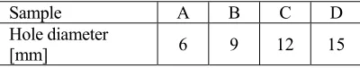
C60 steel (0.6%C, 0.25%Si, 0.75%Mn) bars of 30 mm diameter are cut down into cylinders with a length of 60 mm. Then, holes of various diameters are drilled on those specimens. The specimens are labeled as shown in Table 1. Holes on the specimens were closed before heat treatment in order to avoid contact with the quenchant on the inner surface. This will minimize the heat loss from inner surface and those surfaces are assumed to be insulated for the simulation purpose.

Table 1. Set of specimens used (30 mm diameter, 60 mm length)

During heat treatment, to minimize the danger of distortion and cracking, all specimens were preheated at 200°C for 20 minutes. Then, they were soaked for 30 minutes at the heat treating temperature in a salt bath to prevent decarburization and to ensure uniformity of the temperature and microstructure throughout the entire volume. After austenization, the samples were quenched into water at 20°C. Avoidance of decarburized layer on the surface is essential since the verification of the simulation is based on a comparison of surface residual stresses.

X-ray measurements were carried out on a

Ψ diffractometer using Cr-Kα radiation on a set of crystallographic planes. Since the peak shift due to lattice strains at high diffraction angles is considerably higher, peak having high indices and intensity is preferred for measurements. The intensity and angular position data for analysis is provided by scintillation detector and scaler. Counting has undertaken for a fixed time of 2 s at 2θ angles between 152o _{to 160}o _{by 0.1}o _steps. Parabola method was used for the determination of the peak maximum and position. Then, the corresponding values for interplanar spacing and strains are calculated. Finally, the stress was determined by linear regression analysis by determining the slope of the regression line of lattice strain versus sin2_{ψ plot and multiplying it} with elastic modulus of the material. To minimize the instrumental error, adjustment of the measurement system and effect of specimen curvature on the results were checked by several tests measuring the residual stress on iron powder. To control the reliability and reproducibility of the results, residual stresses were measured repeatedly at the same points on a selected specimen.

In the simulation to improve the efficiency and the stability of the solution, only the required part of the specimen is considered by using the symmetry approach. 3600 (60 in axial, 60 in radial direction) axisymmetric quadrilateral elements were used to create the FE mesh. Mesh was refined near the outer surface in order to improve the accuracy of the solution. Due to very large temperature gradients and early phase transformations, those regions are critical for solution accuracy and convergence.

Initially, the temperature is set to 8300_C for all nodes and all of the elements were assumed to consist of 100% homogeneous austenite. Non-linear convective heat transfer boundary condition was imposed on outer surface which is in contact with the quenchant beside the thermal and mechanical symmetry boundary conditions on the symmetry plane. Surface of the hole is assumed to be insulated. Convective heat transfer coefficient data as a function of surface temperature is presented in Table 2.

Table 2. Variation of heat transfer coefficient with temperature [24]

Temperature [°C] 0 200 400 430 500 560 600 700 800

h [J/(m2_{sK)] 4350 8207 11962 13492 12500 10206 7793 2507 437}

Sample A B C D

Hole diameter

Table 3. Thermo-mechanical material data for C60 steel [24] Austenite

T [°C]

E [GPa] [-] ν

σY [MPa]

H

[MPa] [10α-6_{/K] [W/(mK)]} λ _[106 _J/(mρ.cp 3_K)]

0 200 0.29 220 1000 15.0 4.15

300 175 0.31 130 16000 18.0 4.40

600 150 0.33 35 10000 21.7 4.67

900 124 0.35 35 500

21.7

25.1 4.90 Ferrite, Pearlite, Bainite

0 210 0.28 450 1000 49.0 3.78

300 193 0.30 230 16000 41.7 4.46

600 165 0.31 140 10000 34.3 5.09

900 120 0.33 30 500

15.3

27.0 5.74 Martensite

0 200 0.28 1750 1000 43.1 3.76

300 185 0.30 1550 16000 36.7 4.45

600 168 0.31 1350 10000 30.1 5

900 124 0.35 35 500

13.0

25.1 4.90

A selection of proper time walk procedure is essential for the solution of this highly non-linear system of equations. A convergence analysis was carried out to ensure the convergence at minimum cost. Constant 0.01 sec time steps are used in the analysis according to convergence analysis results. Analysis is terminated when all the nodal temperatures are equal to the quenchant temperature (20°C). Thermo-mechanical data is given in Table 3.

A comparison of simulation results with XRD tangential residual stress measurements is presented in Fig. 1. It can be concluded that the simulation results show good agreement with experimental measurements both in terms of the trends and the magnitude of residual stresses.

To understand the physical origin of residual stresses during quench hardening, heat transfer, phase transformation and mechanical phenomena from the start till the end of process must be carefully traced. Residual stress state depends on both, the thermal stresses and phase transformation stresses. However, phase transformation stresses are usually larger than the thermal ones. Thus, a consideration of cooling rates and sequence of phase transformations at critical stages may provide the engineers to predict the sign and the order of magnitude of the residual stresses without the need of performing numerical simulations: In general, the larger the time difference between phase transformations at

two equilibrating regions, the larger the developed stresses.

Fig.1 . Comparison of the tangential residual stress values (FE simulation and X-Ray

diffraction results)

Critical stages for the development of internal stresses during the quenching process can be summarized as:

Stage 1: It starts at the beginning of quenching and lasts as the phase transformations start. Austenite cools down at different rates at different regions. An internal stress state is developed due to the differences in thermal contraction rates and rates of variation of thermo-mechanical properties, Fast cooling regions are loaded in tension, whereas slow cooling regions are loaded in compression. Stage 2: It begins as the phase transformations start.

transformation plasticity. This leads to unloading and reverse loading on transforming regions while the untransformed regions react to balance those stresses. Transforming regions are loaded in compression whereas the untransformed regions are loaded in tension.

Stage 3: It starts with the transformation of untransformed regions from the previous stage. The already transformed regions experience thermal contraction as they cool down, whereas, the transforming regions expands due to transformations. Similar to the previous stage, this causes an unloading and reverse loading. The already transformed regions are loaded in tension while the transforming regions are loaded in compression.

Stage 4: Austenite is almost completely transformed into different transformation products and thermal stresses are generated

as the specimen cools down. However, those stresses are not so significant because of small temperature gradients.

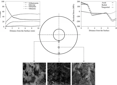
Fig. 2 illustrates the comparison of the microstructure of the specimen B observed in SEM with the one predicted by FE simulation. Predicted axial, radial and tangential residual stress distribution is also presented in the same figure.

From the micrograph it is seen that the outer surface (a) consists of mostly martensite, few bainite/pearlite and trace amount of ferrite. Simulation results report 85% martensite, 10% pearlite and 5% bainite for the same region. Similarly, the mid section (b) is made up of mostly pearlite/martensite mixture, some bainite and few amount of ferrite. 50% pearlite, 33% martensite, 10% bainite and 2% ferrite is predicted for the same region by computer simulation. Finally, the inner surface (c) has a pearlitic microstructure with some martensite/bainite and an increased amount of

ferrite whereas computer simulation results indicate nearly 55% pearlite, 27% martensite, 14% bainite and 4% ferrite. These results indicate a good match between the predicted and observed microstructures.

4 CONCLUSION

A FEM based model was developed, and integrated into commercial FEA software Msc.Marc® by user subroutines. It is capable of predicting temperature history, evolution of microstructure and internal stresses for steel quenching.

The model was verified by simulating the quenching of hollow steel cylinders. The application problem involves transient heat transfer with internal heat source/sink, a small strain thermo-elasto-plastic formulation with phase transformations and anisothermal JMAK phase transformation kinetics. Simulation results were justified with SEM observations and XRD residual stress measurements.

According to the results, it can be concluded that the model can effectively predict the trends in the distribution of the microstructure and residual stresses. The accuracy of prediction is also remarkable. The application problem clearly demonstrates that the determination of final properties of the product after thermal material processing is a challenging task. Even minor changes in the geometry or material properties result in large variations in the microstructure and residual stress distribution. Prediction of the as-quenched state currently necessitates the running of time consuming full scale simulations. However, the authors believe that Fourier analysis of dimensionless parameters involved may reveal most important parameters in the evolution of microstructure and internal stresses.

5 REFERENCES

[1] Şimşir, C., Gür C.H. (2009) Simulation of quenching, Chapter 9, Handbook of Thermal Process Modeling of Steels (Eds: Gür, C.H. Pan, J.) CRC Press-Taylor & Francis, p. 341-425.

[2] Scheil, E. (1935) Incubation timr of the

austenite transformation, Arch.

Eisenhüttenwes vol. 8, p. 565-567. (in German)

[3] Cahn, J.W. (1956) Transformation kinetics

during continuous cooling, Acta

Metallurgica, vol. 4, no. 6, p. 572-575. [4] Christian, J.W. (1975) The Theory of

Transformations in Metals and Alloys

Pergamon Press, Oxford.

[5] Denis, S., Farias, D., Simon, A. (1992) Mathematical model coupling phase transformations and temperature evolutions in steels, ISIJ International, vol. 32, no. 3, p. 316-325.

[6] Lusk, M., Jou, H.J. (1997) On the rule of additivity in phase transformation kinetics,

Metallurgical and Materials Transactions A-Physical Metallurgy and Materials Science,

vol.28, no. 2, p. 287-291.

[7] Reti, T., Horvath, L., Felde, I. (1997) A Comparative study of methods used for the prediction of nonisothermal austenite

decomposition, Journal of Materials

Engineering and Performance, vol.6, no. 4, p. 433-442.

[8] Todinov, M.T. (1998) Alternative approach to the problem of additivity, Metallurgical and Materials Transactions B-Process Metallurgy and Materials Processing Science, vol.29, no. 1, p. 269-273.

[9] Reti, T., Felde, I. (1999) A non-linear extension of the additivity rule,

Computational Materials Science, vol. 15, no. 4, p. 466-482.

[10] Rometsch, P.A., Starink, M.J., Gregson, P.J. (2003) Improvements in quench factor

modelling, Materials Science and

Engineering A, vol. 339, no. 1-2, p. 255-264. [11] Serajzadeh, S. (2004) Modelling of

temperature history and phase transformations during cooling of steel,

Journal of Materials Processing Technology,

vol. 146, no. 3, p. 311-317.

[12] Hsu, T.Y. (2005) Additivity hypothesis and effects of stress on phase transformations in steel, Current Opinion in Solid State & Materials Science, vol.9, no. 6, p. 256-268. [13] Jahanian, S., Mosleh, M. (1999) The

mathematical modeling of phase transformation of steel during quenching,

[14] Kamat, R.G., Hawbolt, E.B., Brimacombe, J.K. (1988) Diffusion modeling of pro-eutectoid ferrite growth to examine the principle of additivity, Journal of Metals,

vol.40, no. 7, p. A52-A52.

[15] Kang, S.H., Im, Y.T. (2005) Three-dimensional finite-element analysis of the quenching process of plain-carbon steel with phase transformation, Metallurgical and Materials Transactions A, vol.36A, no. 9, p. 2315-2325.

[16] Kuban, M.B., Jayaraman, R., Hawbolt, E.B., Brimacombe, J.K. (1986) An assessment of the additivity principle in predicting continuous-cooling austenite-to-pearlite transformation kinetics using isothermal transformation data, Metallurgical Transactions A, vol. 17, no. 9, p. 1493-1503. [17] Nordbakke, M.W., Ryum, N., Hunderi, O.

(2002) Non-isothermal precipitate growth and the principle of additivity, Philosophical Magazine A, vol. 82, no. 14, p. 2695-2708. [18] Reti, T. (2004) On the physical and

mathematical interpretation of the isokinetic hypothesis, Journal De Physique Iv, vol. 120, p. 85-91.

[19] Johnson, W.A. and Mehl, R.F. (1939) Reaction kinetics in processes of nucleation and growth, Trans. AIME, vol.135, p. 416-458.

[20] Koistinen, D.P., Marburger, R.E. (1959) A general equation prescribing the extent of the austenite-martensite transformation in pure

ıron-carbon alloys and plain carbon steels,

Acta Metallurgica, vol.7, no. 1, p. 59-60.

[21] Todinov, M.T. (1998) Mechanism for formation of the residual stresses from quenching, Modelling and Simulation in Materials Science and Engineering, vol. 6, no. 3, p. 273-291.

[22] Belytscko, T., Liu, W.K., Moran, B. (2000)

Nonlinear Finite Elements for Continua and Structures, John Wiley & Sons, Chicester. [23] Simo, J.C., Hughes, T.J. R. (1997)

Computational Inelasticity, Springer-Verlag, New York.

[24] Gür, C.H., Tekkaya, A.E. (2001) Numerical investigation of non-homogeneous plastic deformation in quenching process, Materials Science and Engineering A-Structural Materials Properties Microstructure and Processing, vol.319, p. 164-169.

[25] Judlin-Denis, S. (1987) Modeling of stressphase transformation interactions and finite element calculation of internal stresses during quenching, PhD thesis, Inst. Nat. Polytechnique de Lorraine, France. (in French)

[26] Denis, S., Boufoussi, M., Chevrier, J.C., Simon, A. (1994) Analysis of the development of residual stresses for surface hardening of steels by numerical simulation : effect of process parameters, International Conference on "Residual Stresses" (ICRS4), p. 513-519.