DOI:10.22059/poll.2017.230145.265
Print ISSN: 2383-451X Online ISSN: 2383-4501 Web Page: https://jpoll.ut.ac.ir, Email: [email protected]
Two-dimensional advection-dispersion equation with depth-
dependent variable source concentration
Chatterjee, A. and Singh, M.K.*
Department of Applied Mathematics, Indian Institute of Technology (Indian School of Mines), Dhanbad-826004, Jharkhand, India
Received: 5 Apr. 2017 Accepted: 29 Jun. 2017
ABSTRACT: The present work solves two-dimensional Advection-Dispersion Equation (ADE) in a semi-infinite domain. A variable source concentration is regarded as the monotonic decreasing function at the source boundary (x=0). Depth-dependent variables are considered to incorporate real life situations in this modeling study, with zero flux condition assumed to occur at the exit boundary of the domain, i.e. its semi-infinite part. Without losing any generality, one can consider that the aquifer is initially contamination-free. Thus, the current study explores variations of two-dimensional contaminant concentration with depth throughout the domain, showing them graphically. Non-point source problem, i.e. the line source problem, can be discussed by solving two-dimensional depth-dependent variable source problem, as x=0 is a 2D line. A new transformation has been used to transform the time-dependent ADE to one with constant coefficients, with Matlab (pdetool) being employed in order to solve the problem, numerically, using finite element method.
Keywords: Solute transport, Aquifer, Line source, Numerical solution.
INTRODUCTION
Groundwater is being contaminated in several ways, including industrial effluents, municipal garbage, cemeteries, mine spoils, etc. During past few decades, there have been various studies on groundwater contamination at local as well as global scales by the groundwater scientists, geo-environmentalists, civil engineers, hydrologists etc. The problem of longitudinal dispersion in porous media is solved analytically, where the impacts of flows without any uniformity and variable dispersion coefficients are taken into consideration (Gelher & Collins, 1971).
In the analysis of one-dimensional solute transport through porous media with spatial
Corresponding author, Email: [email protected]
variables retardation factor is under discussion (Chrysikopoulos et al., 1990). Scale-dependent dispersion and periodic boundary conditions have been presented for solute transport in porous media (Logan, 1996), while solute transport in saturated porous media with semi-infinite or finite thickness has been solved analytically (Sim & Chrysikopoulos, 1999).
media, using the discontinuous finite element method, has been discussed (Diwa et al., 2001). And for groundwater flow and radionuclide transport in a single fracture, analytical solutions have been explored with diffusion in surrounding rock matrix, using the symmetry reduction method (Saied & Khalifa, 2002).
An analytical solution for transient, unsaturated transport of water and contaminants through horizontal porous media has been presented with a range of analytical solutions, using similarity solutions for contaminant transport in unsaturated flow, derived using scale and time-dependent dispersivity (Sander & Braddock, 2005). Both analytical solution for transportation of decaying solutes in rivers with transient storage and first-order decay for non-conservative solutes, have been derived (Smedt, 2006). For pore-scale modeling of transverse dispersion in porous media, there has been a comparative study of transverse dispersion, experimenting on a range of Peclet numbers to successfully predict the tendency of the asymptotic macroscopic dispersion coefficient (Bijeljic & Blunt, 2007).
Analytical solutions for sequentially-coupled one-dimensional reactive transport problems have been found (Srinivasan & Clement, 2008), and the one-dimensional analytical solution has been explored by means of Laplace transform technique with suitable initial and boundary conditions (Singh et al., 2009), as well as Laplace Transform Technique (Jaiswal et al., 2011). One-dimensional ADE with variable coefficients was solved analytically (Sander & Braddock, 2005; Singh et al., 2008; Chen & Liu, 2011; Chen et al., 2012a; 2012b). Analytical solutions of non-linear and variable-parameter transport equations for verification of numerical solvers were presented (Zamani & Bombardelli, 2013). The contaminant concentration prediction along unsteady groundwater flow was discussed (Singh & Kumari, 2014). The
ADE has been solved analytically for contaminant transport in the main fracture, surrounded by 2D matrix, in which parallel plate and cylindrical geometry are taken into consideration (Khalifa, 2003). Radial ADE with real life application has been considered and solved, analytically (Lai et al., 2016).
Numerical solution of complicated problems is frequently obtained by researchers and scientists all around the globe. One-dimensional solute transport equation is solved numerically, using finite element and finite difference methods, which have then been compared with one another (Van Genuchten, 1982). Moreover, the numerical correction for finite difference solution of advection and dispersion with reaction has been discussed and compared (Ataie-Ashtiani et al., 1996) and one-dimensional ADE has been addressed in open channel with steady non-uniform flow (Ahmad et al., 1999), where in order to get the numerical results, finite difference and Crank-Nicolson methods were adopted for advection and diffusion processes, respectively. Numerical solution of contaminant transport through unsaturated porous media by means of element free Galerkin method has been taken into consideration (Kumar et al., 2007), with an unconditionally stable finite element (FEM) approach developed to solve the one-dimensional FADE, based on Caputo definition of fractional derivative that has singularity at the boundaries (Huang et al., 2008). The simulation results could be improved by using the third kind of boundary with a fractional-order derivative as the inlet boundary condition. A semi analytical solution has been presented, which is based on the numerical solution for the transportation of conservative and non-reactive tracer (Zhang et al., 2012).
solute transport in porous media in geochemistry, geomorphology, and carbon cycling (Hunt & Ghanbarian, 2016). The contamination, dependent on the time and/or space, was considered by previous researchers (Singh et al., 2009; Singh & Kumari, 2014; Singh et al., 2015) and analytic solutions were derived for aqueous and solid phase colloid concentrations in a porous medium, where colloids are subject to advective transport and reversible retention, dependent on time and/or depth (Leij et al., 2016). A fully-coupled depth-integrated model was considered and solved for surface water and groundwater flow; however, it differed from this problem (Li et al., 2016).
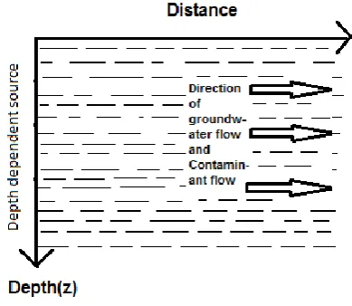
It is interesting to observe the case in hydrological aspects when the source is depth dependent variable, for as the depth increases or decreases, the source may vary too, accordingly, showing some impacts on the aquifer system. This variable source problem was explored too, as a non-point line-source problem, likely to be interesting for researchers who work on groundwater problems and Vedas zone hydrology. The velocity of groundwater was considered unsteady with solute transport occurring only in positive direction of x-axis, i.e. not against the direction of the flow. Matlab (pdetool) was used to solve the problem numerically, using finite element method. Figure 1 illustrates the physical model of the problem.
Fig. 1. Model of the system
MATHEMATICAL FORMULATION A depth-dependent variable source of contamination was considered through the z-axis, i.e. the inlet boundary, shown in Fig.1. A flux type boundary condition was taken into account at the semi-infinite extent (x z, ) of the aquifer, i.e., at the outlet boundary. The aquifer, itself, was initially contamination-free. A function g z( )c e0 z
was considered to describe the source concentration at x= 0 and z>0, so this source acted throughout the depth axis, demonstrated in the Figure 1. It acted like a horizontal line source in inhomogeneous medium. In order to model the contaminant transport in the porous medium and the aquifer aquitard system, ADE was used. Groundwater has specific velocity and dispersion rate along various axes, where dispersion works in every direction of the domain; however, the major part of velocity acts along the x-axis. So in our recent problem we may be able to consider that there is no velocity along the z direction, and it only works in the positive x direction. Nevertheless, dispersion works on both x and z directions, as considered earlier. Two-dimensional ADE was taken into consideration so that the system with time dependent velocity and dispersion coefficient could be modelled. According to hydrology literature, we may manage to assume that dispersion is directly proportional to velocity. Mathematical modeling of the two-dimensional system is as follows:
2 2
2 z 2 ( )
x
C C C C
D D u T
T x z x
(1)
The initial and boundary conditions are as follows:
( , z, ) 0, 0, , 0,
C x T T x z (2)
( , z, ) ( ), 0, z 0, 0,
C x T g z x T (3)
0and 0 when ,
C C
x z
x z (4)
and
x z
D D for time-dependent dispersion along x and z directions, respectively. Furthermore, u(T') represents the velocity of the medium, transporting the solute particles along x axis, as we considered that it was on velocity, along z direction; c0 is constant.
Numerical solution
Both velocity and dispersion are functions of
time, i.e. uu f T0 ( ) and DxauD f T1 ( ')
with DzbuD f T2 ( '), respectively where a
and b are dispersivities with au0D1 and
0 2
bu D . According to dispersion theory,
dispersion is directly proportional to the velocity. Here f T( ) was regarded as an exponentially-decreasing function, i.e. exp(mT). This present paper also considered a fixed value of m=0.01.
Consider, '
0
( ') '
T
T
f t dt (5)We used (5) on (1)-(4), getting the transform equations as follows:
2 2
0
2 2
1 2
C C C C
D D u
T x z x
(6)
The initial and boundary conditions are as follows:
( , z, ) 0, 0, , 0,
C x T T x z (7)
( , z, ) ( ), 0, z 0, 0,
C x T g z x T (8)
0and 0 when ,
C C
x z
x z (9)
Now we considered the transformation ' exp( ) C C z
and using this transformation on (6)-(9), we got the transform equation as follows: 2 2 2 2 0 2 1 2 2
( 2 )
C C C
D D
T x z
C
u D D C
x
(10)
The initial and boundary conditions are as follows:
( , z, ) 0, 0, , 0,
C x T T x z (11)
0
( , z, ) , 0, z 0, 0,
C x T c x T (12)
0and 0 when ,
C C
C x z
x z (13)
Now equations (10)-(13) become ADE with constant coefficients and constant boundary conditions. As a result, we used Matlab in built function (pdetool) to solve this problem numerically, using finite element method. Where this FEM package implemented piecewise linear finite elements for 2D problems, being intended to accompany "Partial Differential Equations: Analytical and Numerical Methods" (second edition) by Mark S. Gockenbach.
RESULT AND DISCUSSION
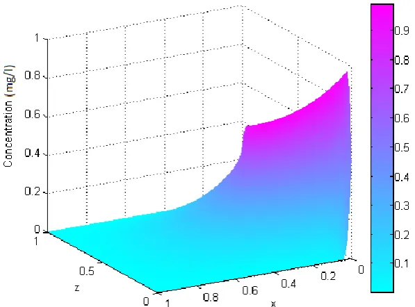
The present work solved two-dimensional ADE, where the source depended on another variable, namely the depth, meaning that the contaminant's contamination decreased or increased with the depth. It was considered that the aquifer was initially contaminant-free. Figure 2 shows initial dispersion D1=
0.1 km2/year and D2= 0.1 km2/year, initial
velocity µ0= 0.09 km/yaer and fixed time t0=
10 year to get the concentration profile with depth and distance. If we consider the change of z, we then see that the contaminant concentration peak is the highest at z=0 and whenever z increases the peak of the concentration declines, accordingly, as the source term is also decreased. From Figure 2, it can also be observed that after a certain distance the contaminant concentration decreased, tending towards zero. It is also clear from Figure 2 that when z as well as x ascended, then the pollutant inflicted more impact, i.e. it took much distance to lose its harmful nature. The contaminant concentration depended on the depth, which can be observed by solving two-dimensional ADE with line source problem, while the contaminant concentration depended on the depth.
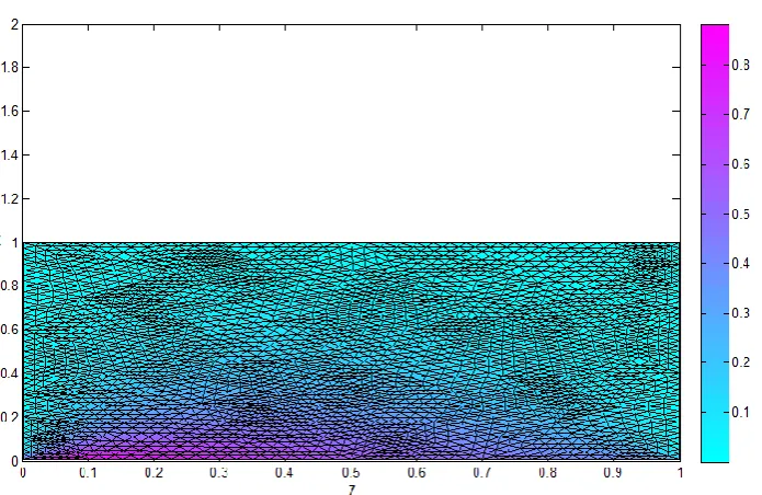
concentration with depth and distance by using contour plotting. It is clear from Figure 3 that near z= 0 km, the contaminant concentration was maximum and after z= 0.7 km, it became negligible. It is also clearly observed from the figure after what distance, we can safely use the groundwater. Both of the concentration
profiles asymptotically tended to zero after a certain distance. It is also observed that although the concentration was higher at the beginning, it was neutralized after some distance and depth. Figure 4 shows the deformation of the domain as mesh/grid and, simultaneously demonstrating the contaminant concentration level.
Fig. 2. Contaminant concentration with depth and distance variables for fixed time t0= 10 years
Fig. 4. Contaminant concentration with depth and distance with deform mesh
Implementation
We can find some real life application of the system, as the contaminant decreased the soil, due to dispersion and gravity, only to lose its contamination level, afterwards. More than 95% of the samples were collected from streams, and almost 50% of them, collected from wells, contained at least one pesticide (Gilliom et al., 1999). The impact of pesticides on streams and groundwater has been discussed where pesticides are commonly found in streams than in groundwater. It has been found that more than 50% of the wells in shallow groundwater and 33% of the deeper wells in major aquifers are contaminated with one or more pesticides (Gilliom, 2007). The authors discussed the mobility and degradation of pesticides in soils as well as the pollution of groundwater resources about the influence of physical and chemical characteristics of the soil on the sorption/desorption and degradation of pesticides and their access to groundwater and surface waters (Arias-Estévez et al., 2008). So it is clear from the study that the waste or contaminants would permeate the soil and these contaminants could behave like a non-point depth-dependent source in the real life situation. Here as we
considered that x= 0 in the boundary condition, the non-point source became line-source. So this concept may be of interest to researchers, working on surface water hydrology or soil contamination problem.
We may present a real life scenario as an example of this type of model. Some industries drown their wastes into the soil, which may in turn mix with the aquifer. After a certain span of time, they drown their wastes into the soil at different depths and subsequently the aquifer may be contaminated with depth-dependent sources, too. There are some contaminants, existing in the atmosphere, undergoing some decay with the depth, which can also be modeled using this formulation.
CONCLUSION
We may conclude from this study that: 1. By addressing and solving two-dimensional depth-dependent source problem via finite element method, it can be shown that depth-dependency affects groundwater contamination problem, which is not yet considered.
we consider the source is acting entirely on the z axis, which is a line source.
3. The peak of contaminant
concentration can be reduced significantly after a certain distance and it may be further reduced to a constant value.
Acknowledgment
The authors are thankful to Indian Institute of Technology (Indian School of Mines), Dhanbad for providing financial support to Ph.D. candidates under the JRF scheme.
REFERENCES
Ahmad, Z., Kothyari, U.C. and Ranga Raju, K.G. (1999). Finite difference scheme for longitudinal dispersion in open channels. J. Hydraul. Research, 37(3): 389-406.
Arias-Estévez, M., López-Periago, E., Martínez-Carballo, E., Simal-Gándara, J., Mejuto, J.C. and García-Río, L. (2008). The mobility and degradation of pesticides in soils and the pollution of groundwater resources. Agriculture, Ecosystems & Environment, 123(4): 247-260.
Ataie-Ashtiani, B., Lockington, D.A. and Volker, R.E. (1996). Numerical correction for finite difference solution of the advection dispersion equation with reaction. J. Contam. Hydrol., 23: 149-156.
Benson, A.D., Wheatcraft, S.W. and Meerschaert, M.M. (2000). Application of a fractional advection-dispersion equation. Water Resour. Res., 36(6): 1403-1412.
Bijeljic, B. and Blunt, M.J. (2007). Pore-scale modeling of transverse dispersion in porous media. Water Resour. Res., 43; W12S11, doi: 10.1029/2006WR005700.
Chen, J.S. and Liu, C.W. (2011). Generalized analytical solution for advection-dispersion equation in finite spatial domain with arbitrary time-dependent inlet boundary condition. Hydrol. Earth Sys. Sci., 15:2471-2479.
Chen, J.S., Lai, K.H., Liu, C.W. and Ni, C.F. (2012a). A novel method for analytically solving multi-species advective-dispersive transport equations sequentially coupled with first-order decay reactions. J. Hydrol., 420-421(14): 191-204.
Chen, J.S., Liu, C.W., Liang, C.P. and Lai, K.H. (2012b). Generalized analytical solutions to sequentially coupled multi-species advective-dispersive transport equations in a finite domain subject to an arbitrary time-dependent source
boundary condition. J. Hydrol., 456-457(16): 101-109.
Chrysikopoulos, C.V., Kitanidis, P.K. and Roberts, P.V. (1990). Analysis of one dimensional solute transport through porous media with spatially variable retardation factor. Water Resour. Res., 26(3): 437-446.
Diwa, E.B., Lehmann, F. and Ackerer, Ph. (2001). One dimensional simulation of solute transfer in saturated-unsaturated porous media using the discontinuous finite element method. J. Contam. Hydrol., 51(3-4): 197-213.10
Gelher, L.W. and Collins, M.A. (1971). General analysis of longitudinal dispersion in non uniform flow. Water Resour. Res., 7: 1511-1521.
Gilliom, R.J. (2007). Pesticides in US streams and groundwater. Environmental Science & Technology, 41(10): 3408-3414.
Gilliom, R.J., Barbash, J.E., Kolpin, D.W. and Larson, S.J. (1999). Peer reviewed: testing water quality for pesticide pollution. Environmental Science & Technology, 33(7): 164A-169A.
Huang, Q., Huang, G. and Zhan, H. (2008).A finite element solution for the fractional advection dispersion equation. Advances in Water Resources, 31: 1578-1589.
Hunt, A.G. and Ghanbarian, B. (2016). Percolation theory for solute transport in porous media: Geochemistry, geomorphology, and carbon cycling. Water Resour. Res., 52(9): 7444-7459.
Jaiswal, D.K., Kumar, A., Kumar, N. and Singh, M.K. (2011). Solute transport along temporally and spatially dependent flows through horizontal semi-infinite media: dispersion proportional to square of velocity. J. Hydrol. Engg., 16(3): 228-238.
Khalifa, M.E. (2003). Some analytic solutions for the advection-dispersion equation. Appl. Math comput., 139: 299-310.
Kumar, R.P., Dodagoudar, G.R. and Rao, B.N. (2007). Meshfree modeling of one dimensional contaminant transport in unsaturated porous media. Geomechanics and Geoengineering: An International Journal, 2(2): 129-136.
Lai, K.H., Liu, C.W., Liang, C.P., Chen, J.S., & Sie, B.R. (2016). A novel method for analytically solving a radial advection-dispersion equation. J. Hydrol., 542: 532-540.
Pollution is licensed under a "Creative Commons Attribution 4.0 International (CC-BY 4.0)"
Li, Y., Yuan, D., Lin, B. and Teo, F.Y. (2016). A fully coupled depth-integrated model for surface water and groundwater flows. J. Hydrol., 542: 172-184.
Logan, J.D. (1996). Solute transport in porous media with scale-dependent dispersion and periodic boundary conditions. J. Hydrol., 184(3-4): 261-276.
Saied, E.A. and Khalifa, M.E. (2002). Analytical solutions for groundwater flow and transport equation. Transp. Porous Media., 47: 295-308.
Sander, G.C. and Braddock, R.D. (2005). Analytical solutions to the transient, unsaturated transport of water and contaminants through horizontal porous media. Adv. Water Res., 28: 1102-1111.
Sim, Y. and Chrysikopoulos, C.V. (1999). Analytic solution for solute transport in saturated porous media with semi-infinite or finite thickness. Adv. Water Res., 22(5): 507-519.
Singh, M.K. and Kumari, P. (2014). Contaminant concentration prediction along unsteady groundwater flow. Modelling and Simulation of Diffusive Processes, Series: Simulation Foundations, Methods and Applications. Springer, XII; 257-276.
Singh, M.K., Mahato, N.K. and Kumar, N. (2015). Pollutant’s Horizontal Dispersion Along and Against Sinusoidally Varying Velocity from a Pulse Type Point Source. Acta Geophysica, 63(1): 214-231.
Singh, M.K., Singh, V.P., Singh, P. and Shukla, D.
(2009). Analytical solution for conservative solute transport in one dimensional homogeneous porous formations with time dependent velocity. J. Engg. Mech., 135(9): 1015-1021.
Singh, M.K., Mahato, N.K. and Singh, P. (2008). Longitudinal dispersion with time dependent source concentration in semi-infinite aquifer. J. Earth Syst. Sci., 117(6): 945-949.
Smedt, F.D. (2006). Analytical solution for transport of decaying solutes in rivers with transient storage. J. Hydrol., 330(3-4): 672-680.
Srinivasan, V. and Clement, T.P. (2008). An analytical solution for sequentially coupled one-dimensional reactive transport problems Part-I: Mathematical Derivations. Water Resour. Res., 31: 203.
Van Genuchten, M.Th. (1982). A comparison of numerical solutions of the one dimensional unsaturated-saturated flow and mass transport equations. Adv. Water Resour., 5: 47-55.
Zamani, K. and Bombardelli, F.A. (2013). Analytical solutions of nonlinear and variable-parameter transport equations for verification of numerical solvers. Environ. Fluid Mech., doi: 10.1007/s10652-013-9325-0.