Numerical solution of variational problems via Haar wavelet quasilinearization technique

Numerical solution of variational problems via Haar wavelet

quasi-linearization technique

Mohammad Zarebnia∗

Department of Mathematics, University of Mohaghegh Ardabili, 56199-11367 Ardabil, Iran. E-mail: [email protected]

Hosein Barandak Imcheh

Department of Mathematics, University of Mohaghegh Ardabili, 56199-11367 Ardabil, Iran. E-mail: [email protected]

Abstract In this paper, a numerical solution based on Haar wavelet quasilinearization (HWQ) is used for finding the solution of nonlinear Euler-Lagrange equations which arise from the problems in calculus of variations. Some examples of variational problems are given and outcomes compared with exact solutions to demonstrate the accuracy and efficiency of the method.

Keywords. Calculus of variation, Boundary value problem, Haar wavelet, Quasilinearization.

2010 Mathematics Subject Classification. 34L99, 34K28, 65T60.

1. _Introduction

The problem of determination a function which maximizes or minimizes a certain functional is called variational problem. In the general form, the variational problems are considered as

φ[u1(t), u2(t), ..., u1(t)] = ∫ t1

t0

F(t, u1(t), u2(t), ..., un(t), u ′ 1(t), u

′ 2(t),

..., u′_n(t))dt,

(1.1)

subject to the boundary conditions for all functions

u1(t0) =α1, u2(t0) =α2, · · ·, un(t0) =αn, (1.2)

u1(t1) =β1, u2(t1) =β2, · · ·, un(t1) =βn. (1.3)

Received: 9 July 2016 ; Accepted: 9 January 2017. ∗Corresponding author.

Here the functional ofφfor the extremum must be found. The necessary condition for this work is to satisfy the Euler-Lagrange equations that is obtained by applying the well known procedure in the calculus of variation [7]

∂F ∂ui

− d

dt( ∂F

∂u′_i) = 0, i= 1,2,· · ·, n, (1.4)

with the boundary conditions given by Eqs. (1.2)-(1.3). The Euler-Lagrange equation (1.4) is generally nonlinear, which does not always have an analytic solution.

Variational problems have been studied extensively by engineers and scientists. These problems arise in a variety of forms in science, engineering and many other various branches of real life, such as economics, mechanics, biology and etc. [7, 10]. Several numerical algorithms have been applied for the solution of problems in the calculus of variations. For example, the Ritz method [7], Laguerre series [10], Galerkin method [5], Walsh series method [3], Chebyshev series [8], and homotopy-perturbation method (HPM) [1] have been used to solve the variational problems. Also Haar wavelet direct method has been applied to variational problems by Hsiao [9]. Sinc-Galerkin method and parametric quintic spline method are also applied for approxi-mating the solution of problems in calculus of variations in [18,19], respectively.

In this article, we will use the Haar wavelet quasilinearization (HWQ) approach for solving the nonlinear problems which arise from problems of calculus of variations. Application of HWQ approach to boundary value problems is investigated in [12]. This method is applied for solving fractional nonlinear differential equations in [17]. In [11,13], nonlinear Lane Emden equations and Burgers’ equation have been solved by applying the HWQ approach. Also the apply of this technique is presented in [14] for solving nonlinear oscillator equations. Convergence of HWQ approach has been given in [14,17].

The balance of this paper is organized as follows: First, in Section 2 we define gen-eral concepts of Haar wavelets. Haar wavelet quasilinearization approach is employed for solving nonlinear boundary value problems in Section 3. In Section 4, we report our numerical outcomes and illustrate the accuracy and efficiency of the presented numerical algorithm by considering four numerical examples.

2. _{Haar wavelets}

Numerical solution of differential equations using Haar wavelets is very efficient due to the following features, simpler and quick, flexible, comfortable, small compu-tational costs and compucompu-tationally attractive.

Theith Haar wavelet hi(t) on the interval [a, b] defined as [16]

hi(t) = {

1, t∈[γ1(i), γ2(i)], −1, t∈[γ2(i), γ3(i)], 0, otherwise,

(2.1)

γ1(i) =a+ 2κσ∆ξ, γ2(i) =a+ (2κ+ 1)σ∆ξ,

γ3(i) =a+ 2(κ+ 1)σ∆ξ, σ=M/m.

The integerm= 2j_{, j= 0,1, ..., J indicates the level of the wavelet. κ= 0,1, ..., m−1}

is the translation parameter. The integerJ determines the maximal level of resolu-tion. We take for the quantity M = 2J _{and ∆ξ = (b−a)/(2M). The index i is}

calculated from the formulai=m+κ+ 1.

We have considered the integral of Haar wavelets as operational matrix [14]. In the general form, the operational matricesρi,α(t) are defined as

ρi,α(t) =             

0, a≤t≤γ1(i),

1 α!

[

t−γ1(i)]α, γ1(i)≤t≤γ2(i),

1 α!

[( t−γ1(i)

)α

−2(t−γ2(i)

)α]

, γ2(i)≤t≤γ3(i),

1 α!

[(

t−γ1(i))α−2(t−γ2(i))α+(t−γ3(i))α], γ3(i)≤t≤b.

(2.2)

The described sequence{hi}∞i=0 is a complete orthonormal system inL2[a, b]. The

orthogonality feature allows us to convert anyφ∈L2[a, b] into Haar wavelets series as

φ(t) =

∞ ∑

i=0

αihi(t) =α0h0(t) + ∞ ∑

j=0 2∑j−1

κ=0

α2j+κh2j+κ(t), t∈[a, b], (2.3)

where

α0= ∫ 1

0

h0(t)φ(t)dt, α2j_+κ= 2j ∫ 1

0

h2j_+κ(t)φ(t)dt. (2.4)

Similarly the highest derivative can be approximated as wavelet series∑∞_i=0αihi(t).

For our purpose, we use the truncated Haar wavelet series as

φ(t)≈

2m ∑

i=0

αihi(t), t∈[a, b]. (2.5)

3. Description of presented technique

Consider thenth order nonlinear ordinary differential equation (1.1) with boundary conditions (1.2) and (1.3). By applying the quasilinearization technique [2], we obtain the (r+ 1)th iterative approximation to the solution Eq. (1.1) as follows

D(n)ur+1(t) =φ(ur(t), u(1)r (t), u (2) r (t), u

(3)

r (t), ..., u (n₋1) r (t), t)

+φ(us)(ur(t), u(1)r (t), u(2)r (t), u(3)r (t), ..., u(rn−1)(t), t)

× n_∑−1

s=0

(u(_rs₊₁) (t)−u(rs)(t)),

whereu(0)r =ur(t) andD(n)is annth order linear ordinary differential operator. The

functionsφ(us)=∂

s_φ

∂us are functional derivatives of the functions.

Now by applying the Haar wavelet approximation, we assume that the highest deriv-ative can be expressed in terms of the Haar wavelet series as

u(_rn₊₁)(t) =

2m ∑

i=0

aihi(t). (3.2)

Then using the concept of operational matrix and Haar wavelet technique, we can obtain the functionsu(_rk₊₁) (t), k= 0,1,2, ..., n−1 from the following equation

u(_rn₊₁−k)(t) =

2m ∑

i=0

aiρi,k(t) + k−1 ∑

i=0

(u(_rn₊₁−k+i)(0)×(t

i

i!)), k= 1,2, ..., n.

(3.3)

Having used each iteration of quasilinearization approach we can get the following linear differential equation

2m ∑

i=0

aihi(t) =φ(ur(t), u(1)r (t), u (2) r (t), u

(3)

r (t), ..., u (n−1) r (t), t)

+φ(_us)(ur(t), u(1)r (t), u (2) r (t), u

(3)

r (t), ..., u (n₋1) r (t), t)

× n ∑

k=1 [(k_∑−1

i=0

(u(_rn₊₁−k+i)(0)×(t

i

i!))

) −

n₋1 ∑

s=0

u(_rs)(t)].

(3.4)

The values of unknown coefficients ai are obtained by solving the linear equation

(3.4). Then, we can get the Haar wavelet quasilinearization (HWQ) solution of Eq. (1.1) by using Eq. (3.3).

4. _{Numerical examples}

In order to illustrate the efficiency of the HWQ method and the performance of the method, the following examples are considered. The examples have been solved by the presented method with level of resolutionJ = 4 and 2m= 32. Note that we have computed the numerical results by Mathematica 10 programming.

Example 1: We first consider the following brachistochrone problem [4]

minφ=

∫ 1

0 [

1 +u′2(t) 1−u(t)

]2

dt, (4.1)

subject to the boundary conditions

The exact solution of this problem in the implicit form is [1]

F(t, u(t)) =−√−u2_{(t) + 0.381510869u(t) + 0.618489131} −t+ 0.5938731505−0.8092445655

×arctan

(

u(t)−0.1907554345

√

−u2_{(t) + 0.381510869u(t) + 0.618489131} )

.

(4.3)

The corresponding Euler-Lagrange equation of the brachistochrone problem is as fol-lows

u′′(t) = 1 2

1 +u′2(t)

1−u(t) . (4.4)

By using the Taylor series, we can write the nonlinear term 1

1−u(t) in (4.4) as follows

1

1−u(t) ≈1 +u(t)−u

2_{(t). (4.5)}

Considering the Eq. (4.5), we can rewrite the Euler-Lagrange equation (4.4) in the following form

u′′(t) = 1 2

(

1 +u(t) +u2(t) +u′2(t) +u(t)u′2(t) +u(t)2u′2(t)). (4.6)

According to the quasilinearization process to (4.6), we get the following linear equa-tion

u(2)_r+1(t) =1 2

[

1 +ur+1(t) +u2r(t) +u (1) r

2

(t) +ur(t)u(1)r 2

(t)(1 +ur(t) )

+(ur+1(t)−ur(t) )(

2ur(t) +u(1)r 2

(t)(1 + 2ur(t) ))

+(u(1)_r+1(t)−u(1)_r (t))(2u(1)_r (t) + 2ur(t)u(1)r (t) (

1 +ur(t) ))]

.

(4.7)

Now by using the Haar wavelet technique to Eq. (4.7), we approximate the term u(2)_r+1(t) by the Haar wavelet series as

u(2)_r+1(t) =

2m ∑

i=0

aihi(t). (4.8)

Integrating (4.8) and using the boundary conditions (4.2), we have

u(1)_r+1(t) =

2m ∑

i=0

aiρi,1(t)− 2m ∑

i=0

aiρi,2(1)−0.5, (4.9)

ur+1(t) = 2m ∑

i=0

aiρi,2(t)−t( 2m ∑

i=0

Substituting Eqs. (4.8)-(4.10) into Eq. (4.7), we get

2m ∑

i=0

aihi(tι) =

1 2

[

1 +

2m ∑

i=0

aiρi,2(tι)−tι (_∑2m

i=0

aiρi,2(1) + 0.5 )

+u2_r(tι)

+u(1)_r 2(tι) +ur(tι)u(1)r 2

(tι) (

1 +ur(tι) )

+(

2m ∑

i=0

aiρi,2(tι)

−tι (_∑2m

i=0

aiρi,2(1) + 0.5 )

−ur(tι) )(

2ur(tι) +u(1)r 2

(tι)

(

1 + 2ur(tι) ))

+(

2m ∑

i=0

aiρi,1(tι)−tι 2m ∑

i=0

aiρi,2(1)−0.5

−u(1)_r (tι) )

×(2u(1)_r (tι) + 2ur(tι)u(1)r (tι) (

1 +ur(tι) ))]

.

(4.11)

Where the collocation points aretι= ι₋1

2

2m, ι= 1,2, ....2m. By taking the

approxi-mate solution for initial function asur(tι) =−tι/2, we compute the values ofu. The

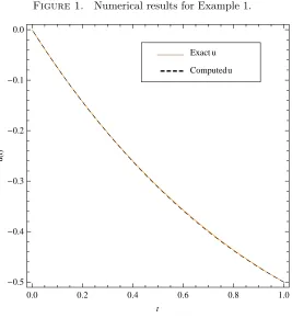
approximate solution of Eq. (4.6) is compared with exact solution and the results are shown in Figure1.

Example 2: Consider the following variational problem [5]

minφ=

∫ 1

0 [

1 +u2_(t)

u′2(t)

]2

dt, (4.12)

subject to the following boundary conditions

u(0) = 0, u(1) = 0.5, (4.13)

with the exact solutionu(t) = sinh (0.4812118250t).

The corresponding Euler-Lagrange equation of this problem is as follows

u′′(t) +u′′(t)u2(t)−u(t)u′2(t) = 0, (4.14)

or equivalently

u′′(t) = u(t)u

′2

(t)

1 +u2_(t). (4.15)

By using the Taylor series, the nonlinear term_1+u12_(t) of the Eq. (4.15) can be written as

1

1 +u2_(t)≈1−u

2_{(t) +u}4_{(t). (4.16)}

Considering the Eq. (4.16), we can rewrite the Euler-Lagrange equation (4.15) in the following form

Figure 1. Numerical results for Example 1.

Computedu Exact u

ÖÖÖÖ ÖÖÖÖ ÖÖÖÖ ÖÖÖÖ

0.0 0.2 0.4 0.6 0.8 1.0

-0.5 -0.4 -0.3 -0.2 -0.1

0.0

t

u

H

t

L

According to the quasilinearization process to (4.17), we get the following linear equa-tion

u(2)_r+1(t) =(u(1)_r+1(t)−u(1)r (t) )(

2ur(t)u(1)r (t)−2u3r(t)u(1)r (t)

+ 2u5_r(t)u(1)_r (t))+(ur+1(t)−ur(t) )(

u(1)_r 2(t)−3u2_r(t)u(1)_r 2(t)

+ 5u5_r(t)u(1)_r 2(t))+ur(t)u(1)r 2

(t)−u3_r(t)u(1)_r 2(t)

+u5_r(t)u(1)_r 2(t).

(4.18)

Now by using the Haar wavelet technique to Eq. (4.18), we approximate the term u(2)_r+1(t) by the Haar wavelet series as

u(2)_r+1(t) =

2m ∑

i=0

Integrating (4.19) and using the boundary conditions (4.13), we have

u(1)_r+1(t) =

2m ∑

i=0

aiρi,1(t)− 2m ∑

i=0

aiρi,2(1) + 0.5, (4.20)

ur+1(t) = 2m ∑

i=0

aiρi,2(t)−t( 2m ∑

i=0

aiρi,2(1)−0.5). (4.21)

Substituting Eq. (4.19) and Eqs. (4.20) and (4.21) into Eq. (4.18), we get

2m ∑

i=0

aihi(tι) = (_∑2m

i=0

aiρi,2(tι)−tι (_∑2m

i=0

aiρi,2(1)−0.5 )

−ur(tι) )

× (

u(1)r 2

(tι)−3u2r(tι)u(1)r 2

(tι) + 5u5r(tι)u(1)r 2

(tι) )

+

(_∑2m

i=0

aiρi,1(tι)−tι 2m ∑

i=0

aiρi,2(1) + 0.5−u(1)r (tι) )

× (

2ur(tι)u(1)r (tι)−2u3r(tι)u(1)r (tι) + 2u5r(tι)u(1)r (tι) )

+ur(tι)u(1)r 2

(tι)−u3r(tι)u(1)r 2

(tι) +u5r(tι)u(1)r 2

(tι).

(4.22)

By taking the approximate solution for initial function asur(tι) =tι/2, we compute

the values ofu. The approximate solution of Eq. (4.17) is compared with exact solu-tion and the results are depicted graphically in Figure2.

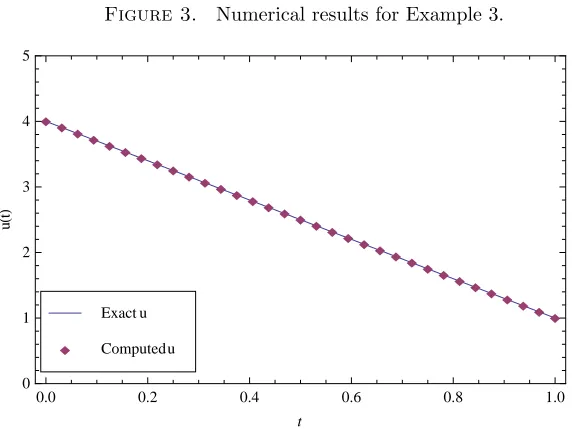
Example 3: In this example we consider the following variational problem with the exact solutionu(t) =(4−3t)in [15]

minφ=

∫ 1

0 (

u′2(t) +u3(t))2dt, (4.23)

subject to the following boundary conditions

u(0) = 4, u(1) = 1. (4.24)

The corresponding Euler-Lagrange equation of this problem is

u′′(t) = 3 2u

2_{(t). (4.25)}

Implementation of the Haar wavelet quasilinearizarion approach to (4.25) gives

2m ∑

i=0

aihi(tι) =3ur(tι) (_∑2m

i=0

aiρi,2(tι)−tι (

3 +

2m ∑

i=0

aiρi,2(1) ) + 4 ) +3 2u 2 r(tι).

(4.26)

By taking the approximate solution for initial function asur(tι) = 0, we compute the

Figure 2. Numerical results for Example 2.

çç

çç

ç

çç

ç

çç

ç

çç

çç

ç

çç

ç

çç

çç

ç ç

ç

çç

ç ç

ç ç

ç

0.0 0.2 0.4 0.6 0.8 1.0

0.0 0.1 0.2 0.3 0.4 0.5

t

u

H

t

L

ç Computedu

Exact u

and the results are shown in Figure3.

Figure 3. Numerical results for Example 3.

ì ì_ì

ì_ì ì

ì_ì ì_ì

ì ì_ì

ì_ì ì

ì_ì ì_ì

ì ì_ì

ì ì_ì

ì_ì ì

ì_ì ì_ì

0.0 0.2 0.4 0.6 0.8 1.0

0 1 2 3 4 5

t

u

H

t

L

ì Computedu

Example 4: Consider the following variational problem [6]

φ(u) = min

∫ 1

0

(1−u(t))(1.05−e1−4u′(t))

(1 +u2_(t))(_{1 +te}−6(t−0.4)2)

(

2

− 1

2(1−u(t))(1 +te−6(t₋0.4)2 )

)

dt,

(4.27)

subject to the following boundary conditions

u(0) = 0.5, u(1) = 0. (4.28)

The corresponding Euler-Lagrange equation of this problem is

∂ ∂u

[

1−u(t) 1 +u2_(t)

1.05−e1−4u′(t)

1 +te−6(t₋0.4)2

4(1−u(t))(1 +te−6(t−0.4)2₎₋₁

2(1−u(t))(1 +te−6(t₋0.4)2 )

] −

d dt

∂ ∂u′

[

1−u(t) 1 +u2_(t)

1.05−e1−4u′(t)

1 +te−6(t₋0.4)2

4(1−u(t))(1 +te−6(t−0.4)2₎₋₁

2(1−u(t))(1 +te−6(t₋0.4)2 )

]

= 0.

(4.29)

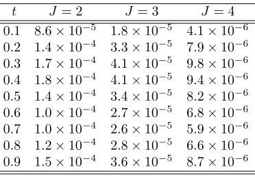
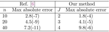
This problem has no exact solution. Since the exact solution of the problem does not exists, we solved the problem for a largeJ and used this approximation as exact solution to compute the errors. The results are tabulated in Table1. Also the our compared results with method in Ref. [6] are given in Table2.

Table 1. Computed absolute errors at different points for Example 4.

t J = 2 J = 3 J = 4 0.1 8.6×10−5 _1.8×10−5 _4.1×10−6

0.2 1.4×10−4 _3.3×10−5 _7.9×10−6

0.3 1.7×10−4 _4.1×10−5 _9.8×10−6

0.4 1.8×10−4 _4.1×10−5 _9.4×10−6

0.5 1.4×10−4 3.4×10−5 8.2×10−6 0.6 1.0×10−4 2.7×10−5 6.8×10−6 0.7 1.0×10−4 2.6×10−5 5.9×10−6 0.8 1.2×10−4 2.8×10−5 6.6×10−6 0.9 1.5×10−4 _3.6×10−5 _8.7×10−6

5. _Conclusion

Table 2. Maximum absolute errors for Example 4.

Ref. [6] Our method n Max absolute error J Max absolute error

10 2.8(-7) 2 1.8(-4)

20 4.5(-9) 3 4.1(-5)

40 7.2(-11) 4 9.8(-6)

illustrative examples.

References

[1] O. Abdulaziz, I. Hashim, and M. S. H. Chowdhury,Solving variational problems by

homotopy-perturbation method, Int. J. Numer. Meth. Engng.75(2008) 709-721.

[2] R. E. Bellman and R. E. Kalaba,Quasilinearization and Nonlinear Boundary Value Problems, American Elsevier Pub. Co. New York, (1965).

[3] C. F. Chen and C. H. Hsiao,it A walsh series direct method for solving variational problems, J. Franklin Inst.300(1975) 265-280.

[4] P. Dayer and S. R. Mcreynolds,The Computation and Theory of Optimal Control, Academic Press, New York, (1970).

[5] L. Elsgolts, Differential Equations and the Calculus of Variations, Mir Publisher, Moscow, (1977).

[6] M. Ghasemi,On using cubic spline for the solution of problems in calculus of variations, Numer. Algor.73(2016) 685-710.

[7] I. M. Gelfand and S. V. Fomin, Calculus of Variations, Prentice-Hall, Englewood Cliffs, NJ, (1963).

[8] I. R. Horng and J. H. Chou,Shifted Chebyshev direct method for solving variational problems, Internat. J. Systems Sci.16(1985) 855-861.

[9] C. H. Hsiao,Haar wavelet direct method for solving variational problems, Math. Comput. Simul. 64(2004) 569-585.

[10] C. Hwang and Y. P. Shih,Laguerre series direct method for variational problems, J. Opt. Theory Appl.39(1983) 143-149.

[11] R. Jiwari,A Haar wavelet quasilinearization approach for numerical simulation of Burgers’

equation, Comput. Phys. Commun.183(2012) 2413-2423.

[12] H. Kaur, R. C. Mittal, and V. Mishra,Haar wavelet quasilinearization approach for solving

nonlinear boundary value problems, Am. J. Comput. Math.3(2011) 176-182.

[13] H. Kaur, R. C. Mittal, and V. Mishra,Haar wavelet approximate solutions for the generalized

Lane Emden equations arising in astrophysics, Comput. Phys. Commun.184(2013) 2269-2277.

[14] H. Kaur, R. C. Mittal, and V. Mishra,Haar wavelet solutions of nonlinear oscillator equations, Appl. Math. Model.38(2014) 4958-4971.

[15] M. L. Krasnov, G. I. Makarenko, and A. I. Kiselev,Problems and Exercises in the Calculus of

Variations, Mir Publisher, Moscow, (1964).

[16] U. Lepik,Solving PDEs with the aid of two-dimensional Haar wavelets, Compu. Math. Appl. 61(2011) 1873-1879.

[17] U. Saeed and M. Rehman, Haar waveletquasilinearization technique for fractional nonlinear

differential equations, Appl. Math. Comput.220(2013) 630-648.

[18] M. Zarebnia and N. Aliniya,Sinc-Galerkin method for the solution of problems in calculus of

[19] M. Zarebnia and Z. Sarvari,Numerical solution of variational problems via parametric quintic