in the population sciences published by the Max Planck Institute for Demographic Research Konrad-Zuse Str. 1, D-18057 Rostock · GERMANY www.demographic-research.org
DEMOGRAPHIC RESEARCH
VOLUME 21, ARTICLE 17, PAGES 503-534
PUBLISHED 16 OCTOBER 2009
http://www.demographic-research.org/Volumes/Vol21/17/ DOI: 10.4054/DemRes.2009.21.17
Research Article
Estimating health expectancies from two
cross-sectional surveys: The intercensal method
Michel Guillot
Yan Yu
© 2009 Michel Guillot & Yan Yu.
This open-access work is published under the terms of the Creative Commons Attribution NonCommercial License 2.0 Germany, which permits use, reproduction & distribution in any medium for non-commercial purposes, provided the original author(s) and source are given credit.
1 Introduction 504
2 Basic principles 508
2.1 Exact relationship linking proportions of “healthy” individuals at two dates
508
2.2 Age-patterns of transition rates in the disability multistate framework
509
2.3 Non-linear model 511
3 Testing the intercensal method using simulations 513
3.1 Generating fictitious population data 513
3.2 Simulating sample data 516
3.3 Constraints, objectives, and starting values in optimization solver 516
3.4 Results 518
3.5 Errors in transition probabilities vs. errors in health expectancies 524
4 Applying the intercensal method to the NHIS 525
5 Discussion 528
6 Conclusion 529
7 Acknowledgments 530
Estimating health expectancies from two cross-sectional surveys:
The intercensal method
Michel Guillot1
Yan Yu2
Abstract
Health expectancies are key indicators for monitoring the health of populations, as well as for informing debates about compression or expansion of morbidity. However, current methodologies for estimating them are not entirely satisfactory. They are either of limited applicability due to high data requirements (the multistate method) or based upon questionable assumptions (the Sullivan method).
This paper proposes a new method, called the “intercensal” method, which relies on the multistate framework using widely available data. The method uses age-specific proportions “healthy” at two successive, independent cross-sectional health surveys, and, together with information on general mortality, solves for the set of transition probabilities that produces the observed sequence of proportions healthy. The system is solved by making realistic parametric assumptions about the age patterns of transition probabilities. Using data from the Health and Retirement Survey and from the National Health Interview Survey, the method is tested against both the multistate method and the Sullivan method. We conclude that the intercensal approach is a promising framework for the indirect estimation of health expectancies.
1 Population Studies Center, University of Pennsylvania, 3718 Locust Walk, Philadelphia PA 19104, USA.
E-mail: [email protected].
2 Australian Demographic and Social Research Institute, The Australian National University, Coombs
1. Introduction
Health expectancies are population health indicators which combine information on both quantity of life (through mortality) and quality of life (usually through disability). Health expectancies measure the number of years that an individual can expect to live in defined health statuses. For example, the life expectancy with disability corresponds to the number of years that one can expect to live with some disability. The disability-free life expectancy corresponds to the number of years that one can expect to live in the absence of disability. Disability and disability-free life expectancies add up to the total, conventional life expectancy.
Health expectancies are important indicators for several reasons. First, they allow the monitoring of the health of populations with a greater level of detail than traditional life expectancies (Mathers et al. 2003). International comparisons of life expectancies may hide important differences in levels of morbidity and disability. This becomes particularly critical as countries advance through the epidemiological transition and experience increasing proportions of deaths due to degenerative diseases often preceded by a period of disability. The World Health Organization has recognized the importance of health expectancies as population health indicators and has estimated them for 191 member states (World Health Organization 2004).
Second, trends in health expectancies are useful indicators for addressing the question of whether current increases in life expectancy are being matched by similar increases in healthy life. In recent decades, several hypotheses have emerged: the expansion-of-morbidity hypothesis, which states that seriously chronically-ill individuals are being kept alive by medical interventions, creating increasing demands on health and social care systems while generating limited improvements in the well-being of the population (Gruenberg 1977; Olshansky et al. 1991); the compression-of-morbidity hypothesis, which states that the average age at onset of disability increases faster than life expectancy, creating a decrease in the number of years spent with disability (Fries 1980, 1983, 1993); and the dynamic-equilibrium hypothesis, an intermediate hypothesis which states that when disability is defined as severe morbidity, the number of years spent with disability remains relatively constant as life expectancy increases (Manton 1982). These are important debates with implications for the future costs of health and social care systems in low-mortality countries. An international research network, the Network on Health Expectancy (Réseau Espérance de Vie En Santé, or REVES), is committed to promoting the use of health expectancies and to improving and harmonizing calculation methods (http://reves.site.ined.fr/en/home/).
of limited applicability because of high data requirements (the multistate method), or based on questionable assumptions (the Sullivan method). The multistate (or increment-decrement) life table method uses a framework that is consistent with the standard life expectancy calculations (Rogers et al. 1990). In a standard period life table, age-specific mortality rates are estimated for one period, and the life expectancy is calculated by simulating a fictitious (or synthetic) cohort of individuals exposed throughout their life time to the mortality rates of that particular period. Thus the period life expectancy summarizes mortality conditions of a particular period. The multistate life table also uses period conditions when calculating the number of years that one can expect to live in a particular health status. Period conditions are summarized with a set of age-specific “transition” rates observed during the period of interest. In the case of health expectancies involving only two health statuses (such as disability-free vs. disabled or, more generally, any “healthy” vs. “unhealthy” dichotomy), there are four possible transitions: from healthy to unhealthy; from healthy to death; from unhealthy to healthy; and from unhealthy to death. Health expectancies are calculated by simulating a synthetic cohort exposed throughout their life time to the transition rates of the period of interest. These health expectancies refer to individuals in a given health state at a given age, and are thus called “conditional” health expectancies. From this simulation are derived “period” or “equilibrium” proportions of healthy individuals, i.e., the proportions of individuals of a given age who are healthy in the synthetic cohort. By weighting conditional health expectancies with these equilibrium proportions, one can obtain “unconditional” health expectancies, i.e., the number of years that one can expect to live above age x in a particular health state, regardless of state at age x.
In spite of its methodological soundness and the richness of its output, the multistate method has one major drawback: it requires data from longitudinal surveys (Mathers 2002). These surveys, which are expensive and complex to carry out, are not widely available. As a result, the multistate method has produced only sporadic health expectancy estimates. These data requirements dramatically reduce the attractiveness of the multistate method, which at present does not appear as a realistic tool for producing long time series of health expectancies or making broad international comparisons of population health (Cambois et al. 1999).
unconditional health expectancies. If the assumption holds, these unconditional health expectancies are equal to the unconditional health expectancies produced by the multistate method. Because of this assumption, the Sullivan method requires only data from one cross-sectional census or survey, together with knowledge of overall mortality (usually an official life table).
However, there is no guarantee that the assumption of the Sullivan method holds in real situations. The currently-observed proportions healthy are the product of a history of mortality and disability that spans about a century, whereas equilibrium proportions are the product of mortality and disability for the current period only. The Sullivan method thus produces an indicator which is affected by the past history of the population (Brouard and Robine 1992). It is not a “pure” period index indicating the number of healthy years that one should expect to live under current conditions. In fact, the Sullivan method can be viewed as a composite method which combines synthetic cohort information (period survival) with actual cohort information (proportions healthy). Another drawback of the Sullivan method is that it produces only estimates of unconditional health expectancies. Age-specific transition rates and conditional health expectancies cannot be estimated with the Sullivan method.
There is some debate in the literature about the magnitude of the bias in the Sullivan method. Some authors have concluded on the basis of actual data that the differences between observed and equilibrium proportions healthy are significant, and that health expectancy estimates based on the Sullivan method should not be used for conclusions on compression or expansion of morbidity (Rogers et al. 1990; Barendregt et al. 1994, 1997; Lievre et al. 2003). On the other hand, Mathers and Robine (1997) have concluded on the basis of simulated scenarios that the differences are not very large and that the Sullivan method is acceptable for monitoring long-term changes in population health. These simulations have been later criticized by Barendregt and colleagues who believe that the chosen scenarios provided too favorable results in support of the Sullivan method (Barendregt et al. 1997). In spite of disagreement about the size of the biases, there is consensus that the multistate method is theoretically sounder than the Sullivan method (Laditka and Hayward 2003) and that one should be careful in interpreting Sullivan-based measures in terms of compression or expansion of morbidity (Nusselder 2003). In sum, it appears that the Sullivan method is the most-commonly used method more because of its reliance on widely available data than because of its reliability. Uncertainties about scenarios of compression or expansion of morbidity may be due in part to these methodological issues.
of period transition probabilities that produces the observed sequence of proportions healthy. The system is solved by making realistic parametric assumptions about the age pattern of transition probabilities. The proposed approach aims at resolving a major drawback of the multistate method by relying on widely available data. Indeed, cross-sectional proportions healthy are widely available from health surveys routinely conducted in various parts of the world and for various time periods, as well as from certain censuses (Myers and Lamb 1992). General mortality information is also widely available. This new approach, which applies when two health statuses (in addition to death) are considered, produces both conditional and unconditional health expectancies.
This is not the first time that two successive cross-sections are used for estimating period conditions. There is a family of indirect demographic methods, called “intercensal” methods, which uses demographic identities to estimate a single-decrement or multiple-single-decrement period life table from two cross-sections (Preston et al. 2001; Schmertmann 2002). The proposed method can be considered as an extension of the intercensal framework to the estimation of a multistate (increment-decrement) life table. We thus refer to this method as an “intercensal” method, although it can use survey data as well.
A number of authors have examined how successive cross-sectional data can be used to estimate a multistate system in the absence of direct information on actual transitions (Willekens 1982, 1999; Schoen and Jonsson 2003). However, the existing approaches (i.e., the Iterative Proportional Fitting (IPF) approach and the Relative State Attraction (RSA) approach) require absolute counts of individuals by state at two cross-sections. They thus have limited applicability when the data come from two independent sample surveys, where the absolute counts of individuals at two cross-sections cannot be related to one-another in a meaningful way. Unlike the IPF and the RSA approaches, the intercensal method does not use absolute counts of individuals as inputs and can thus be applied to data from independent sample surveys. In addition, it makes less constraining assumptions than the RSA approach, especially with regards to mortality (Schoen and Jonsson 2003).
sample surveys with the aim of recovering the multi-state system prevalent during the inter-survey period.
2. Basic principles
2.1 Exact relationship linking proportions of “healthy” individuals at two dates
In this section, the terms “healthy” and “unhealthy” refer to any dichotomous definition of health states. The basic equation of the intercensal approach expresses the observed population proportion of healthy individuals at age x+n and time t+n, Π(x+n, t+n) (=healthy individuals at age x+n and time t+n/all individuals at age x+n and time t+n), in terms of the observed proportion of healthy individuals in the same cohort at time t, Π(x, t), and the transition probabilities prevailing between t and t+n. The derivation of the equation involves following cohorts of healthy and unhealthy individuals between t
and t+n, and comparing their respective evolution to that of the entire cohort, regardless of health status.
Suppose the following transition probabilities, which all refer to conditions of period [t, t+n]:
nqxHU = probability that a healthy individual aged x at time t will be unhealthy at ime
t+n;
nqxHD = probability that a healthy individual aged x at time t will die between time t and t+n;
nqxUH = probability that an unhealthy individual aged x at time t will be healthy at time
t+n;
nqxUD = probability that an unhealthy individual aged x at time t will die between time t and t+n;
nqx = probability that an individual aged x at time t will die between time t and t+n, regardless of health status at age x.
The observed population proportion of healthy individuals at age x+n and time
t+n, Π(x+n, t+n), is equal to:
x n
UH x n HU
x n HD x n
q
q t x q
q t x n t n x
−
⋅ Π − + − − ⋅ Π = + + Π
1
)] , ( 1 [ ) 1
( ) , ( ) ,
( (1)
) ( 1 ) , ( 1 ) , ( 1 1 ) , ( ) , ( HU x n HD x n x n UH x n x n x n q q q t x q q t x q t x n t n
x ⋅ +
− Π − ⋅ − Π − = − Π − + +
Π (2)
By defining nrx = nqxUD/nqxHD (unhealthy/healthy mortality ratio) and using the fact that death probabilities for the entire population are weighted averages of the death probabilities for healthy and unhealthy populations (nqx = Π(x, t) nqxHD + [1-Π(x, t)] nqxUD), Equation (2) can be rewritten as:
HU x n x n x n x n x n UH x n x n x n q q t x r t x t x q q t x q q t x q t x n t n x ⋅ − Π − ⋅ Π − + Π − ⋅ Π − ⋅ − Π − = − Π − + + Π 1 ) , ( )] , ( 1 [ ) , ( ) 1 /( ) , ( 1 ) , ( 1 1 ) , ( ) , ( (3)
If the only available information consists of two independent cross-sections of the population (with age and health status as variables), as well as a conventional life table prevailing between t and t+n, the known quantities of Equation (3) are Π(x, t), Π(x+n, t+n) and nqx. The other quantities, nqxUH, nqxHD, and nrx are unknown. When data are available for k age groups, Equation (3) expands to a system of k equations.
This system of k equations is obviously not solvable, because it has 3*k unknowns. However, the quantities nqxUH, nqxHD, and nrx do not vary randomly with age. On the contrary, they correspond to health processes that are clearly related to age (incidence of disability, recovery from disability, and active/disabled mortality ratio in the case of the active vs. disabled dichotomy). As discussed in the next section, these quantities follow some rather simple functions of age. Knowledge of the age patterns of these three functions will reduce the number of unknowns in the system of equations, and allow us to search for optimal solutions.
2.2 Age-patterns of transition rates in the disability multistate framework
There is a body of literature showing that the four sets of transition rates in the active/disabled/dead multistate framework follow some well-defined age-patterns. For example, Rogers et al. (1990) and Crimmins et al. (1994) have shown that such transition rates are well described by exponential functions at ages 60 and above.
k j x p
q
jk jk j x h
jk x
h = + , ≠
ln α β (4)
where hpxj is the monthly probability of remaining in state j between x and x+h, and where hqxjk is the monthly probability of moving from state j to state k between x and
x+h (j = U, H and k = U, H, D). This age pattern is used as a basis for estimating transition probabilities with the IMaCh procedure, which uses longitudinal data. Lièvre et al. have applied this model to data from the Longitudinal Study on Aging (LSOA) and produced estimates of monthly transition probabilities for the sampled population. We converted these monthly transition probabilities into annual and 2-year probabilities (allowing multiple transitions during the two-year period) and found that these probabilities (i.e., nqxHU, nqxUH, nqxHD, nqxUD for n=1 or n=2) are very well fitted with simple exponential functions at ages 60 and above. This means that exponential assumptions for one or two-year transition probabilities are consistent with Lièvre et al.’s assumptions for monthly transition probabilities.
Our analysis of data from the 1998 and 2000 Health and Retirement Study (HRS) confirms the validity of exponential assumptions for two-year transition probabilities. The 1998 HRS is a nationally representative sample of elderly adults aged 50 and above living in households in the United States in 1998. After deleting 460 cases that were known to be alive but lost; and 63 cases whose survival status was unknown at the 2000 follow-up, the 1998 sample has 10,809 cases (i.e., 4635 men and 6174 women) between the exact age of 64 and 94. Among them, 521 men and 542 women died by the 2000 interview. The analysis does not use sample weights because our preliminary investigation indicates no substantial difference between the un-weighted and weighted data in the age patterns of health state transition probabilities.
We follow the convention of defining the two living states (active and disabled) in terms of functional limitations in the following six activities of daily living (ADLs): dressing, walking across the room, bathing or showering, eating, getting in or out of bed, or using the toilet (Katz et al. 1973). A respondent is defined to be disabled if s/he reported to have any difficulties that last more than three months with at least one of the ADLs, or to "cannot", or "do not do" at least one of them, and to be active if otherwise. In the remainder of this paper, “H” refers to the active state, and “U” refers to the disabled state. Information for month and year of death is available from reports by proxy respondents, or from linkage with the 2000 National Death Index.
the disabled. The four sets of transition probabilities are well fitted by exponential functions of age, as shown by the exponential curves in Figure 1. The observed and fitted age patterns of mortality for active and disabled individuals imply that the ratio of disabled to active mortality (nrx) is greater than one and follows a declining exponential function of age. These results are consistent with Lièvre et al.’s results with the LSOA data.
Figure 1: Observed and fitted age-specific transition probabilities, HRS, 1998-2000 (both sexes combined)
65 70 75 80 85 90
0. 0 0. 1 0.2 0.3 0. 4 0. 5 Age x 2qx H U Observed Fitted
65 70 75 80 85 90
0. 0 0. 1 0.2 0.3 0. 4 0. 5 Age x 2qx H D
65 70 75 80 85 90
01
23456
Age x
2r
x
65 70 75 80 85 90
0. 0 0. 1 0.2 0.3 0. 4 0. 5 Age x 2qx U H
65 70 75 80 85 90
0. 0 0. 1 0.2 0.3 0. 4 0. 5 Age x 2qx U D
Note: H=active (no ADL limitation); U=disabled (at least one ADL limitation); D=Dead.
2.3 Non-linear model
) exp( )
exp( ] 1 [ )
exp( 3 3
2 2 1
1 D x
x C
C
B x
A
Y x
x x
x x
x = α β − + − α β − α β (5)
where
Yx = Π(x+n, t+n) - Π(x, t)/(1 - nqx); Ax = [1-Π(x, t)]/(1 - nqx);
Bx = Π(x, t) nqx /(1 - nqx); Cx = Π(x, t);
Dx = Π(x, t)/(1 - nqx).
Yx, Ax, Bx, Cx and Dx are the known quantities of Equation (3). Equation (5) can be viewed as a model in which a dependent variable, Yx, is related to five independent variables (x, Ax, Bx, Cx, Dx) in a nonlinear fashion.
The core idea of the proposed approach is to use nonlinear optimization techniques to estimate the unknown parameters of Equation (5). Optimization techniques solve systems of equations using iterative procedures. The first step of the optimization consists of defining an “objective” for the optimization, i.e., the quantity that needs to be minimized. The most common objective is the minimization of the sum of squared residuals, but other objectives can be specified. The system is usually solved through a procedure in which initial values of the parameters are iteratively improved until the objective is met (Bates and Watts 1988). In this paper, we use the CONOPT non-linear optimization solver interfaced with the programming language GAMS. This solver is useful for our purpose, because it allows us to specify bounds in the parameters, as discussed below in section 3.3 (Rosenthal 2008).
Once the parameters are solved for, it is possible to produce age-specific estimates of nqxUH, nqxHU and nrx, which, together with knowledge of nqx, are sufficient to recover the full set of period transition probabilities (nqxHU, nqxUH, nqxHD, nqxUD) consistent with the observed changes in proportions active and the observed overall death probabilities. Knowledge of these transition probabilities allows the estimation of a full multistate life table and corresponding period health expectancies (both conditional and unconditional), using classic multistate life table construction techniques (Preston et al. 2001).
would have to involve a rate-to-probability conversion and its associated assumptions. This would substantially increase the complexity of the non-linear estimation process. Given that this method relies on very little input data, with only as many observations as age groups, we decided to rely on the most parsimonious relationship between the known and unknown quantities. The second reason is that the main goal of this method is to estimate health expectancies, which requires knowledge of probabilities. If the method was producing rates, we would still have to perform a rate-to-probability conversion in order to estimate health expectancies. In brief, using rates rather than probabilities would be at once more complex and unnecessary. One disadvantage of working with probabilities, though, is that the metric of probabilities (and, thus, the corresponding parametric assumptions) depend on the length of the age interval. By contrast, the metric of rates computed over discrete age intervals will not differ from that of the underlying continuous process (as long as they are expressed with the same exposure metric such as person-years). Age patterns of rates thus better reflect the underlying continuous process of interest, and can be more easily tailored to the various age interval configurations via the rate-to-probability conversion. We believe, however, that for this particular method, the advantages of working with probabilities outweigh the disadvantages.
In this paper, we test our method using two different strategies. We first rely on simulations, with the goal of testing the method’s ability to recover the parameters that generated the simulated data. We then apply the method to two actual cross-sections from the National Health Interview Survey (NHIS), and compare how the method performs in comparison with the multistate approach based on longitudinal data from the HRS.
3. Testing the intercensal method using simulations
3.1 Generating fictitious population data
In a first series of tests, we generated a fictitious population of active and disabled individuals exposed to known transition probabilities, and tested the method’s performance in the ideal situation where the parametric assumptions are exactly met and where there is no sampling variability.
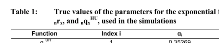
Table 1: True values of the parameters for the exponential functions nqxUH, nrx, and nqxHU, used in the simulations
Function Index i αi βi
nqxUH 1 0.35269 -0.04303
nrx 2 5.50699 -0.04878
nqxHU 3 0.06957 0.05598
Note: These values are based on data from the HRS, 1998 & 2000, for both sexes combined. The functions were fitted using least-squares and a transformed age a=x-65. This age transformation allows to obtain intercepts that correspond to the values of the functions at age 65.
We then generated population proportions of active individuals at time t, Π(x,t), by smoothing the HRS 1998 proportions in two-year age intervals centered at exact age x, between ages 65 and 93, for both sexes combined. (This series is arbitrary; the test could be conducted with any series of proportions active at time t.)
These proportions of active individuals at time t were then projected to time t+2, using equation (1) and the fitted transition probabilities. This step required knowledge of 2qx (total mortality), which we calculated using the fitted mortality curves for the active and the disabled, along with the population proportions active at time t (nqx = Π(x, t) nqxHD + [1-Π(x, t)] nqxUD).
Population proportions of active individuals at time t and t+2 are shown in Table 2, together with the age-specific transition probabilities (including total mortality) that agree with these two cross-sections. The health expectancies that correspond to these age-specific transition probabilities are shown in Table 3. (In order to avoid the use of age extrapolation in these tests, we calculated partial health expectancies at age 65, truncated at age 95.) These are the “true” health expectancies that the new method seeks to estimate.
The population proportions active at time t and t+2 shown in Table 2, together with overall mortality values (nqx), give us all the information to calculate the “known” elements of Equation (5), i.e., Ax, Bx, Cx, Dx, and Yx. We can then use these data as inputs in the optimization solver, with the goal of recovering the original parameters that generated the data and estimating corresponding health expectancies.
Table 2: Population proportions active at time t, transition probabilities between t and t+2, and corresponding proportions active at time t+2 exact
age x Π(x,t) nqxUH nqxUD nqxHU nqxHD nrx nqx Π(x+2,t+2)
65 67 69 71 73 75 77 79 81 83 85 87 89 91 93 0.86269 0.85747 0.85151 0.84341 0.83187 0.81158 0.78091 0.74265 0.69547 0.64174 0.58876 0.54383 0.50863 0.48197 0.46421 0.35269 0.32361 0.29692 0.27244 0.24997 0.22936 0.21045 0.19309 0.17717 0.16256 0.14916 0.13686 0.12557 0.11522 0.10572 0.11036 0.12191 0.13467 0.14876 0.16434 0.18153 0.20053 0.22152 0.24471 0.27032 0.29861 0.32987 0.36439 0.40253 0.44466 0.06957 0.07781 0.08703 0.09734 0.10887 0.12177 0.13620 0.15233 0.17038 0.19056 0.21314 0.23839 0.26663 0.29821 0.33354 0.02004 0.02441 0.02972 0.03620 0.04409 0.05369 0.06539 0.07963 0.09698 0.11811 0.14384 0.17518 0.21335 0.25983 0.31644 5.50699 4.99510 4.53080 4.10965 3.72765 3.38116 3.06687 2.78180 2.52322 2.28869 2.07595 1.88298 1.70796 1.54920 1.40520 0.03244 0.03830 0.04530 0.05382 0.06429 0.07777 0.09498 0.11613 0.14195 0.17262 0.20747 0.24572 0.28754 0.33372 0.38511 0.86177 0.84845 0.83397 0.81745 0.79798 0.77249 0.73990 0.70158 0.65674 0.60665 0.55514 0.50565 0.45793 0.40938 0.35648
Note: nqxUH, nqxUD, nqxHU, and nqxHD are based on fitted data from the HRS, 1998 & 2000, for both sexes combined (See table 1).
Π(x,t) are smoothed age-specific proportions active in the 1998 HRS for both sexes combined.
Table 3: Values of health expectancies (partial health expectancies at age 65, truncated at age 95) for the period t to t+2, by health status at age 65, derived from the fitted transition probabilities shown in Table 2 (H = active; U=disabled; .=active or disabled)
Health status of destination
H U .
H 13.77 3.93 17.71
U 8.73 6.06 14.79
Health status at age 65
. 13.08 4.23 17.31
3.2 Simulating sample data
In reality, even if the parametric assumptions are met in the population, the observed proportions active at two dates may not come from population data but from sample data. It is thus important to introduce sampling variability in the data for a more realistic test of the method’s performance. We thus drew random samples of various sizes from the two population cross-sections generated in the above section. These simulated samples were then used as inputs in the intercensal method, thus testing the method’s performance in a situation where the parametric assumptions are met and where the only source of uncertainty comes from sampling variability.
Specifically, we took the population proportions of active individuals shown in Table 2 as the “true” proportions. At each age group at time t and t+2, each individual was a random draw with the probability of being active equal to the population proportions active. The sample sizes are 20,000, 10,000 and 5,000 individuals in 1998 and 2000, with an age distribution following that of the US population in 1998 and 2000. For each pair of samples, the proportions active at time t and t+2, together with overall mortality values (nqx), were used as inputs in the optimization solver. (No sampling variability was introduced in the overall mortality values, since we expect mortality data to come from official, population-based estimates.) As above, the goal is to recover the original parameters that generated the data and estimate corresponding health expectancies. These estimated health expectancies can be compared to the “true” health expectancies shown in Table 3.
3.3 Constraints, objectives, and starting values in optimization solver
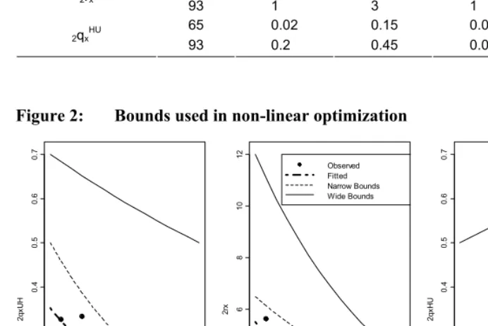
functions nqxUH, nqxHU and nrx, while ensuring that the above constraints are met. We tested two sets of bounds, a narrower one and a wider one. These bounds are provided in Table 4 and shown in Figure 2. Relative to the observed data, the wide bounds include very high and very low levels of the three functions nqxUH, nqxHU and nrx. While we would need to have empirical estimates of transition probabilities in a wide range of contexts to be able to fine tune these bounds, the wide bounds appear large enough to encompass a wide variety of situations.
Table 4: Values of bounds used in optimization procedure
Narrow bounds Wide bounds Function Age
low high low high
65 0.25 0.5 0.1 0.7
2qxUH
93 0.05 0.15 0.02 0.5
65 3.5 6.5 2 12.0
2rx
93 1 3 1 4.0
65 0.02 0.15 0.01 0.5
2qxHU
93 0.2 0.45 0.08 0.7
Figure 2: Bounds used in non-linear optimization
65 70 75 80 85 90
0.
0
0.1
0.
2
0.3
0.
4
0.5
0.
6
0.7
Age x
2q
xU
H
65 70 75 80 85 90
02
46
8
10
12
Age x
2rx
Observed Fitted Narrow Bounds Wide Bounds
65 70 75 80 85 90
0.
0
0.1
0.
2
0.3
0.
4
0.5
0.
6
0.7
Age x
2q
xH
We used the minimum of the sum of squared residuals (min Σx (Ŷx-Yx)2 ) as the objective for the optimization solver. With both narrow and wide bounds, all 1000 samples had locally optimal solutions, which is all that can be guaranteed for a nonlinear model. The convergence took 20 to 30 iterations on average. We used various combinations of starting values for the 6 unknown parameters of Equation (5). Regardless of the choice of starting values, the optimizer always converged to the same solution.
3.4 Results
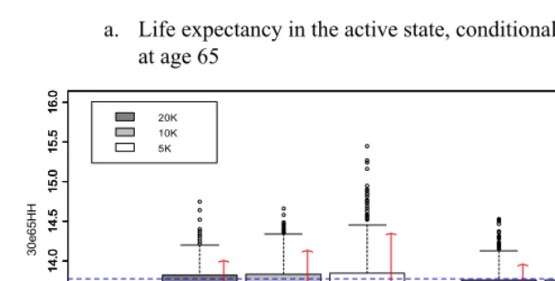
We evaluate the intercensal method by comparing health expectancies estimated with this method to the “true” health expectancies shown in Table 3. Results for each conditional or unconditional health expectancy are presented in Figure 3-5 according to the following configurations: (1) Sample size (20K, 10K or 5K per cross-section); (2) Bounds in nonlinear optimization (narrow, wide). For each combination of these configurations, we present how health expectancies estimates are distributed among 1,000 pairs of samples randomly drawn from the simulated population at time t and t+2. Each sampling distribution is presented in two ways: (1) box plots showing medians and quartiles (boxes represent inter-quartile ranges or IQR, whiskers extend to 1.5 times the IQR below the first quartile or above the third quartile, and estimates beyond that range are considered outliers and are represented by dots); (2) means and 90% uncertainty intervals (means are represented with dots, and whiskers around these dots represent the range between the 5th and 95th percentile).
Figure 3: Simulated sampling distribution of health expectancies at age 65 (in years), conditional on being active at age 65, by sample size and bound width
a. Life expectancy in the active state, conditional on being active at age 65
1 2 13. 0 13. 5 14. 0 14. 5 15. 0 15. 5 16. 0 30e65HH 1 2 13. 0 13. 5 14. 0 14. 5 15. 0 15. 5 16. 0 1 2 13. 0 13. 5 14. 0 14. 5 15. 0 15. 5 16. 0
Narrow (1) or Wide (2) Bounds in Nonlinear Programming
20K 10K 5K
b. Life expectancy in the disabled state, conditional on being active at age 65
1 2 3. 0 3 .5 4. 0 4 .5 30 e6 5 H U 1 2 3. 0 3 .5 4. 0 4 .5 1 2 3. 0 3 .5 4. 0 4 .5
Narrow (1) or Wide (2) Bounds in Nonlinear Programming
Figure 3: (Continued)
c. Life expectancy (any disability state), conditional on being active at age 65
1 2
17.
5
18.
0
18.
5
19.
0
30e65H.
1 2
17.
5
18.
0
18.
5
19.
0
1 2
17.
5
18.
0
18.
5
19.
0
Narrow (1) or Wide (2) Bounds in Nonlinear Programming
20K 10K 5K
Note: These health expectancies are partial health expectancies at age 65, truncated at age 95 (30e65). The horizontal dashed lines
represent the true population health expectancies shown in Table 3.
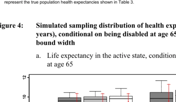
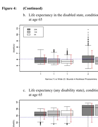
Figure 4: Simulated sampling distribution of health expectancies at age 65 (in years), conditional on being disabled at age 65, by sample size and bound width
a. Life expectancy in the active state, conditional on being disabled at age 65
1 2
4
6
8
10
12
30e6
5U
H
1 2
4
6
8
10
12
1 2
4
6
8
10
12
Narrow (1) or Wide (2) Bounds in Nonlinear Programming
Figure 4: (Continued)
b. Life expectancy in the disabled state, conditional on being disabled at age 65
1 2
5
678
9
1
0
1
1
30e6
5U
U
1 2
5
678
9
1
0
1
1
1 2
5
678
9
1
0
1
1
Narrow (1) or Wide (2) Bounds in Nonlinear Programming
20K 10K 5K
c. Life expectancy (any disability state), conditional on being disabled at age 65
1 2
11
1
2
1
3
14
15
1
6
17
30e
65U
.
1 2
11
1
2
1
3
14
15
1
6
17
1 2
11
1
2
1
3
14
15
1
6
17
Narrow (1) or Wide (2) Bounds in Nonlinear Programming
20K 10K 5K
Note: These health expectancies are partial health expectancies at age 65, truncated at age 95 (30e65). The horizontal dashed lines
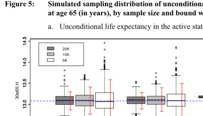
Figure 5: Simulated sampling distribution of unconditional health expectancies at age 65 (in years), by sample size and bound width
a. Unconditional life expectancy in the active state
1 2 3
12 .5 13 .0 13 .5 1 4 .0 1 4 .5 30 e6 5 .H 1 2 12 .5 13 .0 13 .5 1 4 .0 1 4 .5 1 2 12 .5 13 .0 13 .5 1 4 .0 1 4 .5 20K 10K 5K
Narrow (1) or Wide (2) Bounds in Nonlinear Programming & Sullivan Estimates (3)
b. Unconditional life expectancy in the disabled state
1 2 4
3. 5 4 .0 4. 5 5 .0 30 e65. U 1 2 3. 5 4 .0 4. 5 5 .0 1 2 3. 5 4 .0 4. 5 5 .0 20K 10K 5K
Narrow (1) or Wide (2) Bounds in Nonlinear Programming & Sullivan Estimates (3)
Note: These health expectancies are partial health expectancies at age 65, truncated at age 95 (30e65). The horizontal dashed lines
We observe the following patterns in these results. Overall, the intercensal method appears to work remarkably well for health expectancies conditional on being active at age 65 (Figure 3), and for unconditional health expectancies (Figure 5). For these health expectancies, the method offers little bias and sampling error; the means and medians of the sampling distributions are typically within a few decimal points from the true value, and the size of the 90% uncertainty interval rarely extends beyond one year.
There is more bias and more sampling error for health expectancies conditional on being disabled at age 65 (Figure 4), especially when wide bounds are used. For these values, means and medians of sampling distributions are typically within one year of the true values, and uncertainty can be quite substantial. This may be due to the fact that these conditional health expectancies for the disabled are greatly affected by the estimated value of 2qxUH at age 65. Indeed, 2q65UH is high in comparison with the other transition probabilities at that age, which means that small relative errors in the value of that probability (estimated with α1) will have a large impact on the health expectancies conditional on being disabled. On the positive side, errors in these conditional health expectancies have little impact on the unconditional health expectancies shown in Figure 5, because they pertain to a small proportion of the population at age 65.
Comparing different combinations of sample size and bounds, we find the following patterns in terms of bias and sampling error. First, as expected, larger samples produce better results, but the gain is not always substantial. Second, the choice of narrower bounds in the nonlinear optimization provides better results. The gain, however, is not very substantial, except in the case of health expectancies conditional on being disabled at age 65 (Figure 4). For these health expectancies, the use of narrow bounds produces much less bias and sampling error.
In order to test the limits of this approach, we also run the optimization solver with no bounds, keeping only the five constraints specified above. The no bounds results were less satisfactory. First, about 5% of the samples encountered infeasibility and unboundedness. Second, while the IQR and the 90% uncertainty intervals for the feasible solutions were comparable in range to the wide-bounds results, a few solutions, up to 15 out of 1000 samples, had values far outside the range observed. While the non-bounded results are useful to test the limits of the estimation procedure, they put us in an unnecessary difficult situation by ignoring a priori information about the order of magnitude of the functions. For example, it might not be useful to allow the procedure to yield results where the death probability of the active is more than 12 times that of the disabled at age 65. While the proposed narrow and wide bounds could be fine tuned by examining transition probabilities in a wide range of contexts, we believe there is more a priori information to be used than just the five constraints specified above.
3.5 Errors in transition probabilities vs. errors in health expectancies
Since the purpose of this method is to estimate health expectancies, we focused our discussion of the results on errors in this outcome measure. However, transition probabilities are also an outcome of interest for a number of purposes. We observe that probabilities are less accurately estimated than the health expectancies produced by them. Values of nqxHU and nqxUH, in particular, tend to be seriously underestimated. These errors largely offset each other when calculating health expectancies.
Figure 6: Observed and estimated intercensal age-specific transitions probabilities, HRS, 1998-2000
65 70 75 80 85 90 95
0. 0 0.1 0. 2 0.3 0. 4 0.5 Age x 2qx H U
65 70 75 80 85 90 95
0. 0 0.1 0. 2 0.3 0. 4 0.5 Age x 2qx H D
65 70 75 80 85 90 95
012 3 4 5 6 Age x 2r x Observed Intercensal, Narrow Bounds Intercensal, Wide Bounds
65 70 75 80 85 90 95
0. 0 0.1 0. 2 0. 3 0. 4 0. 5 Age x 2qx U H
65 70 75 80 85 90 95
0. 0 0.1 0. 2 0. 3 0. 4 0. 5 Age x 2qx U D
4. Applying the intercensal method to the NHIS
The above simulations provide a test of the intercensal method in situations where the parametric assumptions are exactly met and where the only source of error comes from sampling variability. They do not fully replicate real-life situations where the underlying assumptions might not be exactly met, and where the three sources of information (two cross-sections and overall mortality) come from three independent sources, each with their own potential errors.
Our definition of health states in the NHIS is not identical to the one we used in the HRS. This is due to the fact that, instead of asking about having any difficulty as in the HRS, the NHIS health questions ask about needing help. As the subject may have difficulty in functioning without needing help, the prevalence of functional limitations in the NHIS is generally lower than that in the HRS for the same type of activities. To make the level of prevalence comparable between the two surveys, we expanded the list of activities in the NHIS to include: (1) personal care needs such as eating, bathing, dressing, or getting around inside the home; (2) routine needs such as everyday household chores, doing necessary business, shopping, or getting around for other purposes; and (3) being limited in the kind or amount of work one can do. Cases with a positive response to any of these items were coded as disabled.
For overall mortality pertaining to the inter-survey period, we used U.S. mortality data from the Human Mortality Database for the year 2000. These data are based on official life tables from NCHS. Because of the age restriction in the NHIS, we used 9 age groups only (65-81) as inputs. The input data are shown on Table 5.
Table 5: Proportions active (1999 & 2001) and overall mortality (2000) used as inputs in the intercensal method, US, both sexes combined exact age x Π(x, 1999) Π(x+2, 2001) nqx (2000)
65 67 69 71 73 75 77 79 81
0.87609 0.86819 0.85219 0.83519 0.82684 0.81417 0.77641 0.76045 0.70216
0.86708 0.86906 0.84669 0.82160 0.79093 0.82322 0.75590 0.71198 0.66378
0.03037 0.03590 0.04216 0.04980 0.05958 0.07025 0.08283 0.09915 0.11846
Source: 1999 & 2001 National Health Interview Survey (proportions active); Human Mortality Database (overall mortality).
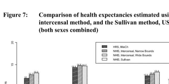
Figure 7: Comparison of health expectancies estimated using IMaCh, the intercensal method, and the Sullivan method, US, 1998-2001 (both sexes combined)
HH HU H. UH UU U. .H .U
HRS, IMaCh
NHIS, Intercensal, Narrow Bounds NHIS, Intercensal, Wide Bounds NHIS, Sullivan
Yea
rs
0
5
10
1
5
20
12 12.713.2
2.4 2.1
1.6
14.414.8 14.7
7.9
6.8
4.2 4.6 6.1
9.2 12.512.9
13.4
11.412 12.1 11.8
2.7 2.6 2.5 2.7
Note: H=Active; U=Disabled; .=Active or Disabled. These health expectancies are partial health expectancies at age 65, truncated at age 83 (18e65). IMaCh estimates are based on data from HRS, 1998 & 2000 waves. Intercensal estimates are based on data
Results indicate that, compared to the IMaCh approach using HRS, the intercensal method provides remarkably comparable estimates for unconditional health expectancies (.H and .U), and for health expectancies conditional on being active at age 65 (HH, HU and H.). For these health expectancies, errors range from .3 to .8 years with narrow bounds; and from .4 to 1.2 with wide bounds. As in our earlier test, the errors are larger for health expectancies conditional on being disabled at age 65, especially when wide bounds are used. Active life expectancy (UH) tends to be underestimated, while life expectancy in the disabled state (UU) tends to be overestimated. These two errors balance out for the total life expectancy conditional on being disabled (U.), producing an error of .4 years when narrow bounds are used, and .9 years when wide bounds are used. These results are consistent with the results of the earlier simulations.
For unconditional health expectancies, we are also able to compare the results of the intercensal method to those of the Sullivan method. The intercensal method and the Sullivan method perform similarly well, with little difference between wide bounds and narrow bounds. Here also, this is consistent with the results of the simulations.
5. Discussion
In light of the simulations and examples developed in this paper, the intercensal approach appears as a promising framework for indirectly estimating health expectancies. In this section, we discuss the advantages and disadvantages of this approach, compared to the two most common approaches that have been used so far: the multistate approach using IMaCh, and the Sullivan method.
The advantages relative to the Sullivan method are many. First of all, unlike the Sullivan approach, the intercensal method allows the estimation of conditional health expectancies. Health expectancies vary substantially depending on one’s health status at a given age, and therefore conditional health expectancies are important health indicators. A second advantage is that the intercensal method, like IMaCh, does not rely on the assumption that the observed prevalence of disability of the population is equal to the that of the synthetic cohort. It is therefore more theoretically correct. Another advantage is that the intercensal method produces unconditional health expectancy estimates that are slightly less biased than those resulting from the Sullivan method. The disadvantage relative to the Sullivan method is that it requires two cross-sections, instead of one in the case of the Sullivan method. This is a minor disadvantage given that successive cross-sections are widely available. A related disadvantage is that the unconditional health expectancies produced by the intercensal method have more sampling variability than the Sullivan method. This additional sampling variability is modest, however, and seems to be an acceptable price to pay in view of the advantages that the intercensal method offers compared to the Sullivan method.
6. Conclusion
The intercensal method developed in this paper allows the estimation of health expectancies (conditional and unconditional) without the use of longitudinal data. It only requires two successive cross-sections of the population and overall mortality pertaining to the inter-survey period. Assumptions regarding the age pattern of transitions are similar to those made by IMaCh.
The intercensal method works perfectly when there is no sampling variability and when parametric assumptions are exactly met in the population. When we introduce sampling variability, the method appears to work remarkably well for estimating health expectancies conditional on being active at age 65, and for unconditional expectancies.
The amount of error is somewhat larger for health expectancies conditional on being disabled at age 65. Fortunately, this is a small population group at age 65, and therefore these errors do not compromise the multistate system and the other health expectancy estimates. Nonetheless, further research is needed for improving the performance of the method for these conditional health expectancies.
would help choosing perhaps more sensible bounds for the values of the parameters. The age pattern of transition probabilities also needs to be studied for various widths of age intervals (e.g. 3 years, 5 years, etc.), and for other healthy vs. unhealthy dichotomies.
We believe, however, that the method introduced in this paper provides a useful framework for estimating health expectancies in the absence of longitudinal data.
7. Acknowledgments
References
Barendregt, J.J., Bonneux, L., and Van Der Maas, P.J. (1994). Health expectancy: an indicator for change? Journal of Epidemiology and Community Health 48(5): 482-487. doi:10.1136/jech.48.5.482.
Barendregt, J.J., Bonneux, L., and Van Der Maas, P.J. (1997). How good is Sullivan's method for monitoring changes in population health expectancies? Journal of
Epidemiology and Community Health 51(5): 578-579.
doi:10.1136/jech.51.5.578.
Bates, D.M. and Watts, D.G. (1988). Nonlinear regression analysis and its
applications. New York: Wiley. doi:10.1002/9780470316757.
Brouard, N. and Robine, J.M. (1992). A method of calculation of health expectancy applied to longitudinal surveys of the elderly in France. In: Robine, J.M., Blanchet, M., and Dowd, J.E. (eds.). Health Expectancy. London: HMSO. Cambois, E., Robine, J.M., and Brouard, N. (1999). Life expectancies applied to
specific statuses: a history of the indicators and the methods of calculation.
Population: an English Selection 53(3): 447-476.
Crimmins, E.M., Hayward, M.D., and Saito, Y. (1994). Changing mortality and morbidity rates and the health status and life expectancy of the older population.
Demography 31(1): 159-175. doi:10.2307/2061913.
Davis, B.A., Heathcote, C.R., and O’Neill, T.J. (2001). Estimating cohort health expectancies from cross-sectional surveys of disability. Statistics in Medicine
20: 1097-1111. doi:10.1002/sim.724.
Fries, J.F. (1980). Aging, natural death, and the compression of morbidity. New
England Journal of Medicine 303(3): 130-135.
Fries, J.F. (1983). The compression of morbidity. Milbank Memorial Fund Quarterly
61(3): 397-419. doi:10.2307/3349864.
Fries, J.F. (1993). Compression of morbidity: life span, disability, and health care costs.
Facts and Research in Gerontology 7: 183-190.
Gruenberg, E.M. (1977). The failure of success. Milbank Memorial fund Quarterly/ Health and Society 55: 3-24. doi:10.2307/3349592.
Imai, K. and Soneji, S. (2007). On the estimation of disability-free life expectancy: Sullivan’s method and its extension. Journal of the American Statistical
Katz, S., Branch, L.G., Branson, M.H., Papsidero, J.A., Beck, J.C., and Greer, D.S. (1983). Active life expectancy. New England Journal of Medicine 309(20): 1218-1224.
Laditka, S.B. and Hayward, M.D. (2003). The evolution of demographic methods to calculate Health expectancies. In: Robine, J.M., Jagger, C., Crimmins, E.M., and Suzman, R.M. (eds.). Determining health expectancies: Hoboken, NJ: Wiley: 221-234.
Laditka, S.B. and Wolf, D.A. (1998). New methods for analyzing active life expectancy. Journal of Aging and Health 10(2): 214-241.
doi:10.1177/089826439801000206.
Lièvre, A., Brouard, N., and Heathcote, C. (2003). The estimation of health expectancies from Cross-longitudinal Surveys. Mathematical Population Studies
10: 211-248. doi:10.1080/713644739.
Manton, K.G. (1982). Changing concepts of morbidity and mortality in the elderly population. Milbank Memorial Fund Quarterly 60(2): 183-244.
doi:10.2307/3349767.
Mathers, C.D. (2002). Health expectancies: A review and appraisal. In: Murray, J.L., Salomon, J.A., Mathers, C.D., and Lopez, A.D. (eds.). Summary Measures of
Population Health. Geneva: World Health Organization: 177-204.
Mathers, C.D. and Robine, J.M. (1997). How good is Sullivan's method for monitoring changes in population health expectancies? Journal of Epidemiology and Community Health 51(1): 80-86. doi:10.1136/jech.51.1.80.
Mathers, C.D., Salomon, J.A., Murray, C.J.L., and Lopez, A.D. (2003). Alternative summary measures of population health. In: Murray, C.J.L. and Evans, D.B. (eds.). Health systems performance assessment: Debates, methods and
empiricism. Geneva: World Health Organization: 319-334.
Myers, G.C. and Lamb, V.L. (1992). Sources of data for assessing healthy life expectancy. In: Robine, J.M., Blanchet, M., and Dowd, J.E. (eds.). Health
Expectancy. London: HMSO: 118-123.
Nusselder, W.J. (2003). Compression of morbidity. In: Robine, J.M., Jagger, C., Crimmins, E.M., and Suzman, R.M. (eds.). Determining health expectancies.
Hoboken, NJ: Wiley: 35-58.
Olshansky, S.J., Rudberg, M.A., Carnes, B.A., Cassel, C.K., and Brody, J.A. (1991). Trading off longer life for worsening health. Journal of Aging and Health 3: 194-216. doi:10.1177/089826439100300205.
Preston, S.H., Heuveline, P., and Guillot, M. (2001). Demography: Measuring and
Rogers, A., Rogers, R., and Belanger, A. (1990). Longer life but worse health? Measurement and dynamics. The Gerontologist 30(5): 640-649.
Rosenthal, R.E. (2008). GAMS - A user's guide. GAMS Development Corporation: Washington D.C., USA.
Schmertmann, C.P. (2002). A simple method for estimating age-specific rates from sequential cross sections. Demography 39(2): 287-310.
doi:10.1353/dem.2002.0018.
Schoen, R. and Jonsson, S.H. (2003). Estimating multistate transition rates from population distributions. Demographic Research 9(1): 1-24.
doi:10.4054/DemRes.2003.9.1.
Sullivan, D.F. (1971). A single index of mortality and morbidity. HSMHA Health Reports 86: 347-354.
Willekens, F. (1982). Multidimensional population analysis with incomplete data. In: Land, K.C. and Rogers, A. (eds.). Multidimensional Mathematical Demography. New York: Academic Press: 43-111.
Willekens, F. (1999). Modeling approaches to the indirect estimation of migration flows: From entropy to EM. Mathematical Population Studies 7: 239-278. World Health Organization (2004). The World Health Report 2004: Changing History.