c
Copernicus GmbH 2003
Advances in
Radio Science
Comparison of errors and stability in FDTD and FVTD
P. Leuchtmann, C. Fumeaux, and D. Baumann
Institut f¨ur Feldtheorie und H¨ochstfrequenztechnik, ETH Z¨urich, CH-8092 Z¨urich, Switzerland
Abstract. The methods of finite-difference time-domain (FDTD) and finite-volume time-domain (FVTD) are well known techniques for solving electromagnetic problems. While for FDTD a number of commercial codes is avail-able there are only few based on FVTD. However, FVTD has advantages since it allows completely unstructured meshes. This paper 1. deals with the principle errors made in both ap-proaches and 2. gives a theoretical comparison of the (local) stability of an FVTD scheme as opposed to the conventional Yee-scheme commonly used in FDTD. Finally the principles of a new FVTD program is presented. Its capabilities are demonstrated by the field of an antenna array.
1 From field functions to numbers
In any numerical technique for solving Maxwell’s equations the vector-valued r, t (space,time) functions E(r, t ) (elec-tric field strength),H(r, t )(magnetic field strength),D(r, t ) (displacement density) andB(r, t )(magnetic flux density) are mapped to a finite set of numbers to be processed by the computer. In the well-known Yee-scheme (Yee, 1966; Taflove and Hagness, 2000) field components are taken at particular locations on a cubic grid such that the component values can be seen as “exact” values at the respective loca-tions and the equaloca-tions applied to these values can be in-terpreted as second-order finite-difference approximations of Maxwell’s equations. E.g., the z-component of Maxwell’s first equation is −∂
∂tBz(r, t ) = ∂
∂xEy(r, t )− ∂
∂yEx(r, t ).
This can be approximated to second-order accuracy at the location(r, t )by
−Bz(+δt)−Bz(−δt) 2δt
≈
Ey(+δx)−Ey(−δx)
2δx
−Ex(+δy)−Ex(−δy) 2δy
(1)
Correspondence to: P. Leuchtmann
whereδx, δy, δz, δt are the respective half grid constants and
sayEy(+δx)is short forEy(x+δx, y, z, t ). This means that
the approximation of this particular component of Maxwell’s equations at the location(r, t ) needs only field values be-ing half space- or time-steps apart from this location. Yee’s scheme uses different locations for different field compo-nents. Fig. 1a shows the spatial location of both the com-ponents and the equations. Note that the material equations (B=µH andD=εE) are easily satisfied for each compo-nent separately at its own location. The Yee-scheme consists of set AY: six Maxwellian component Eqs. (1) plus set BY: six material equations. Set AY is of second-order accuracy, set BYis exactly satisfied.
In the finite integration technique (FIT) (Weiland, 1977) Maxwell’s first equation in integral form (−∂
∂t
RR
AB·dA=
H
∂AE · ds) is applied to the green rectangle shown in
Fig. 1(b). −∂
∂thBziA·2δx·2δy= hEyi
+δx
L ·2δy− hEyi
−δx
L ·2δy−
hExi
+δy
L ·2δx− hExi
−δy
L ·2δx
(2) Therebyh.iδ
L means a line mean value along the respective side of the rectangle andh.iAmeans the surface mean value. After integrating the whole Eq. (2) along the time interval fromt−δt tot+δt and then dividing it by 8δxδyδt we
ob-tain time mean values (denoted by overbars) at the right-hand side and surface mean values evaluated at the boundary of the time interval at the left-hand side:
−hBziA(+δt)− hBziA(−δt) 2δt
=
hEyi
+δx
L − hEyi
−δx
L 2δx
−hExi +δy
L − hExi
−δy
L 2δy
(a) (b) (c)
Fig. 1. The well-known Yee-scheme (a) places different field components at different locations. We use•for magnetic components and for electric components. The respective values are used to form second-order accurate difference equations. The FIT-approach (b) uses mean values (B- andD-components: surface mean values;E- andH-components: line-mean values). In FVTD (c) volume-mean values (B- and D-vectors) and face-mean values (E- andH-vectors) are used.
Fig. 2. The picture shows 988 wave vector directions (from the
sphere’s center). The numerical schemes are tested using plane waves propagating in the respective directions.
valuehBziAwhich is a value at a fixed time. The FIT-scheme consists of set AF: six Maxwellian component equations plus set BF: six material equations. Set AF is exactly satisfied while set BFis approximate.
In the finite-volume time-domain (FVTD) approach Maxwell’s equations can also be integrated over a volume V rather than a surface A as done in the FIT-derivation in the previous section. We assume a polyhedron V withN sur-faces Fiforming the boundary∂V of V (see Fig. 1c) and find,
e.g.,
−∂ ∂t
ZZZ V
BdV
| {z }
V·hBiV
= − ZZ ⊂⊃
∂V
E×dA=
N
X
i=1 ni×
ZZ Fi
EdA
| {z }
Fi·hEiFi
, (4)
wherehEiF
i andhBiV are the time-dependent mean values
of the vector functionsE(orB) on the polyhedronsi-th face Fi (or the volume respectively) andni is the respective outer
normal unit vector. Hence Eq. (4) is an exact relation be-tween time dependent mean values. If Eq. (4) is integrated
over time an exact vector-valued equation somehow similar to Eq. (3) is found:
−hBiV(+δt)− hBiV(−δt) 2δt
= 1 V
N
X
i=1
Fi ni× hEiFi
. (5)
Using Maxwell’s second equation another exact vector equa-tion involvinghDiVandhHiF
i values is obtained.
Concerning time the face mean values are “older” than the newest volume mean value at the left hand side. “Newer” face mean values might be obtained by the extrapolation hEiF(t+2δt)≈2hEiF(t+δt)− hEiF(t ),
hHiF(t+2δt)≈2hHiF(t+δt)− hHiF(t ). (6) Since each face has two sides one can set up further relations, e.g.
hHiF ≈wl
µlhBiVl+
wr
µrhBiVr
hEiF ≈wl
εlhDiVl+
wr
εrhDiVr
or even hHiF≈f hBiVl,hBiVr,hDiVl,hDiVr
hEiF ≈g hBiV
l,hBiVr,hDiVl,hDiVr
(7) where the indices r and l stand for “left” and “right” (of the face F) respectively. The quantities wr,l are some weights due to geometry. In a simple symmetrical case (two identical cells) it iswr = wl = 1
2. In the more complicated case,f andgare some functions yet to be specified. Regardless of the particular choices both Eqs. (6) and (7) are approximate relations.
FVTD ends up with an exact set AV of six scalar Eq. (5) and a second set BV – formed with Eqs. (6) and (7) – of approximate relations.
0.2 0.4 0.6 0.8 1. 20
40 60 80 100 120 140
(a) 0.2 0.4 0.6 0.8 1.
20 40 60 80 100 120 140
(b) 0.2 0.4 0.6 0.8 1.
50 100 150 200
(c)
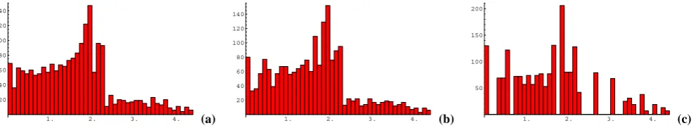
Fig. 3. The histograms of the FIT-errors according to Eq. (10) for2λδ
ξ =14. . .15 (cells per wave length). Maximum values are around 1%.
From left to rightηFITx,ηFITyandηFITzare shown.
1. 2. 3. 4. 20
40 60 80 100 120 140
(a) 1. 2. 3. 4.
20 40 60 80 100 120 140
(b) 1. 2. 3. 4.
50 100 150 200
(c)
Fig. 4. Histograms of the FVTD-errors according to Eq. (11) for2λδ
ξ =14. . .15 (cells per wave length). Maximum values are around 4%
which is four times more than in FIT. This higher value is not a principle drawback of FVTD but mainly due to our simple choice in Eqs. (6) and (7): essentially a first order scheme both in space and time. From left to rightηFVTDx,ηFVTDyandηFVTDzare shown.
with a large matrix Mmet hod where “method” is one out of
FDTD, FIT and FVTD:
[V]new=Mmet hod· [V]old. (8)
Two questions can be posed:
Accuracy: “To what degree are the approximate equations
wrong in each case?”
Stability: “Under what conditions are the respective schemes numerically stable?”
Since FDTD and FIT differ only in the interpretation of the numbers but lead to formally the same equations we treat only the FIT.
2 The definition of the errors and their values
The accuracy depends on several things such as structure and dimension of the mesh but also on the actual field. We define 988 test cases of the actual field: plane waves propagating in different directions. A single plane wave in a homogeneous medium is described by
D(r, t )/ε=E(r, t )=E0·cos(ωt−κ·r) B(r, t )/µ=H(r, t )=H0·cos(ωt−κ·r) with H0=
1
ωµκ×E0,κ·E0=0, κ·κ =ω
2µε. (9)
The directions ofκ := (κx, κy, κz)andE0are free beside these restrictions.
Given one of these test fields[V]oldis computed for both methods in the respective way (space and/or time mean val-ues) and also the respective exact[V]new,ex. A slightly
dif-ferent value for[V]newis obtained by using Eq. (8). A com-parison of[V]new,exand[V]newdelivers the respective error. In order to keep the amount of computation within reason-able limits we restrict the error analysis to the approximative equations and use typical discretisation lengthsδξ (fractions
of the wavelengthλ= 2|π
κ|).
In FIT the material equations are approximate relations, e.g., hDξiA ≈ εhEξiL. From this we derive the error rEx := εhEξiL/hDξiA
!
= 1. Introducing the expressions given in Eq. (9) and evaluating the mean values by analytical integration we find a value different from 1 for the respective exact ratio:
˜
rEx= Si(κxδx)·Si(κyδy) Si(κzδz)·Si(ωδt)
⇒ηFITx:= | ˜rEx−1|·100% (10) with Si(x) := sinx
x . The histograms of these error values
evaluated forδx =δy=δz=
q 3
µεδtand all wave directions
shown in Fig. 2 are given in Figs. 3 and 4.
In order to obtain a reasonable basis of comparison we use a regular cubic grid (with 2δx·2δy·2δz-cubes) also in the
FVTD case and make the aforementioned simple choices in Eqs. (6) and (7). Moreover we can setw1=w2= 1
2. Intro-ducing the expressions from Eq. (9) and performing the inte-grations according to the definitions in the FVTD-formulae we finally obtain for the update equation related to a face oriented inξ-direction
ηFVTDξ :=2
Si(2κξδξ)−Si(2ωδt)
Si(ωδt)
·100% (11)
3 The stability
The time iterative scheme is a repeated application of Eq. (8). This means that the matrix Mmet hod should not have any
eigenvalue λ with |λ| > 1. For a full problem the di-mension of Mmet hod is very large and the respective search
for all eigenvalues would be extremely expensive. How-ever, there are special numerical schemes (e.g., the Arnoldi scheme) which find the largest eigenvalue within still rea-sonable time. In this work we do not follow that way but reduce the number of variables (and with it the dimension
of Mmet hod) by defining a local stability by focusing on a
single cell. Considering the update scheme for a particular value (e.g., by solving Eq. 3 or 5 for the latestB-value) we find that for computing all “new” values of a single cell the number of the required “old” values is always larger than the number of “new” values. This simply reflects the fact that “old” values from the neighbour cells are also involved. The respective ‘local’ update equation would have a small
but rectangular matrix Mlocal. This matrix can be reduced
to a quadratic matrix by applying a spatial Fourier transfor-mation to the “old” values. In this case any “old” value can be written asvold,0·ej (κxx˜+κyy˜+κzz)˜ where vold,0is the value in the cell’s center, (x,˜ y,˜ z)˜ denotes the displacement and κ =(κx, κy, κz)is the vector of the spatial Fourier
frequen-cies. In particular values required from outside the cell are related to the respective values inside the cell by a simple multiplication with the respective dislocation factor.
The restriction of the stability analysis to a single Fourier term is sufficient if stability is proofed for any Fourier term. This can be deduced from Parseval’s theorem: the sum of all Fourier terms (which is the true field) remains stable.
Note that in the rectangular grid neighbour values are sim-ply multiplied bye±j κξδξ which remains true even for line-,
surface- and volume mean values. Assuming a homogeneous material in and around the cell in FIT/FDTD the (6× 6)-matrix M can be written as
H E new =
U+µε1MEMH µ1ME
1
εMH U
| {z }
M · H E old (12) with U=
1 0 0 0 1 0 0 0 1
,
ME=
0 δt
δz(e
2j κzδz−1) −δt
δy(e
2j κyδy −1)
−δt
δz(e
2j κzδz−1) 0 δt
δx(e
2j κxδx −1)
δt
δy(e
2j κyδy −1) −δt
δx(e
2j κxδx −1) 0
,
MH =
0 −δt
δz(1−e
−2j κzδz) δt
δy(1−e
−2j κyδy)
δt
δz(1−e
−2j κzδz) 0 −δt
δx(1−e
−2j κxδx)
−δt
δy(1−e
−2j κyδy) δt
δx(1−e
−2j κxδx) 0
.
(13)
The eigenvalues’ amount of M does not exceed 1 if and only if δt2
µε ≤
1
sinδxκx
δx
2
+sinδyκy
δy
2
+sinδzκz
δz 2 ≤ 1 1 δx 2 +1
δy
2 +1
δz
2 =↑
δx=δy=δz=δ
δ2
3 . (14)
This is the well-known Courant limit.
In FVTD there are 24 scalar variables per cell: 3 face mean valuesE1,2,3andH1,2,3plus volume mean values ofBandD. The scheme can be written as
[E1 E2 E3 H1 H2 H3 B D]Tnew=M·[E1 E2 E3 H1 H2 H3 B D]Told (15) with the 24×24-matrix
M=
−U 0 0 1+αx
ε Ax
1+αx
ε Ay
1+αx
ε Az 0
1+αx
ε U
0 −U 0 1+εαyAx
1+αy
ε Ay
1+αy
ε Az 0
1+αy
ε U
0 0 −U 1+αz
ε Ax
1+αz
ε Ay
1+αz
ε Az 0
1+αz
ε U
−1+αx
µ Ax −
1+αx
µ Ay −
1+αx
µ Az −U 0 0
1+αx
µ U 0
−1+αy
µ Ax −
1+αy
µ Ay −
1+αy
µ Az 0 −U 0
1+αy
µ U 0
−1+αz
µ Ax −
1+αz
µ Ay −
1+αz
µ Az 0 0 −U
1+αz
µ U 0
−Ax −Ay −Az 0 0 0 U 0
0 0 0 Ax Ay Az 0 U
where 0 stands for a 3-by-3 zero-matrix,αx:=ej κxδx,αy:=ej κyδy,αz:=ej κzδz and
Aξ =
δt
δξ
(1−1/αξ)Kξ, Kx =
"0 0 0 0 0 −1
0 1 0
#
, Ky =
" 0 0 1
0 0 0
−1 0 0
#
, Kz=
"0 −1 0
1 0 0
0 0 0
#
. (17)
Evaluating the eigenvalues of M yields
−1,+1,± v u u u t1−γ δ
2
t
µε± v u u
t 1−γ δ 2
t
µε !2
−1 with γ = 1−cos 2κxδx δ2
x
+1−cos 2κyδy δ2
y
+1−cos 2κzδz δ2
z
(18)
We find that forγ δt2/(µε)≤2 all eigenvalues are unimodular complex numbers while forγ δt2/(µε) >2, there are eigenvalues with an absolute value being larger than one. A stability-criterion is therefore
1 δx2+
1 δy2 +
1 δ2z ≤
µε
δt2 (19)
This is exactly the same as Eq. (14) in FIT/FDTD!
4 The FVTD program
A FVTD program is developed in parallel to this theoretical study. To take advantage of the geometrical flexibility of the method, the FVTD algorithm is applied in an unstructured tetrahedral mesh. This type of mesh permits a conformal meshing of complicated geometries including, e.g. curved or oblique surfaces.
The basic FVTD Eq. (4) is numerically integrated in each cell of the mesh in a time-stepping iteration. The approx-imate relations of the type Eq. (7) are implemented
us-ing the followus-ing approach: For each face of the cell only the field components tangential to the face are considered (plane-wave ansatz) and the fields are split into incoming and outgoing contributions. Second-order accuracy in space is achieved using the MUSCL approach (monotonic upwind scheme for conservation laws (Bonnet et al., 1999)) that in-terpolates volume values (assumed located in the barycenter of the cell) to face centers using estimated gradients.
When using second-order accurate schemes in space, the first-order time-stepping scheme of the left side of Eq. (5) is advantageously replaced by the second-order
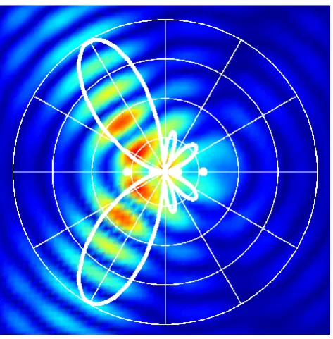
predictor-Fig. 5. A four element linear array of Hertzian dipoles (white dots on the horizontal axis). The near-zone E-field (magnitude distribution) is
corrector Lax-Wendroff scheme (Bonnet et al., 1999). This scheme permits as alternative to Eq. (6) to obtain “newer” face mean values in the numerical estimation of Eq. (5). The resulting implemented algorithm is consequently second-order accurate both in space and time. Absorbing boundary conditions of the Silver-M¨uller type or Engquist-Majda type are applied to the outer boundary of the computational do-main.
Figure 5 shows the nefield distribution of a linear ar-ray of four elementary dipoles with half-wave spacing. The plane of observation is perpendicular to the dipoles and lo-cated slightly above them. This example validates the FVTD method for EM simulations. The modeling of complicated structures requires only a geometrical definition and mesh-ing of the structure but no change in the FVTD algorithm. Application of the FVTD method to more complicated ex-amples is in progress.
5 Conclusions
Common numerical schemes may involve significant errors in particular equations. The FVTD-schemes have many
de-grees of freedom. The simple scheme treated here leads to unacceptably high errors. However, it is expected that a more sophisticated scheme delivers much lower errors.
References
Yee, K. S.: Numerical solution of initial boundary value problems involving maxwell’s equations in isotropic media, IEEE Trans-actions on Antennas and Propagation, 14(3): 302–307, 1966. Taflove, A. and Hagness, S. C.: Computational
Electrodynam-ics – The finite-difference time-domain method, Artech House, Boston, 2nd edition, 2000.
Weiland, T.: A discretization method for the solution of maxwell’s equations for six-component fields, Electronics and Communi-cations AE ¨U, 31: 116–120, 1977.