Dynamic data-driven model reduction: adapting reduced models from incomplete data

R E S E A R C H A R T I C L E

Open Access

Dynamic data-driven model reduction:

adapting reduced models from

incomplete data

Benjamin Peherstorfer

and Karen Willcox

*_{Correspondence:} [email protected]

Department of Aeronautics and Astronautics, MIT, 77 Massachusetts Avenue, Cambridge 02139, USA

Abstract

This work presents a data-driven online adaptive model reduction approach for systems that undergo dynamic changes. Classical model reduction constructs a reduced model of a large-scale system in an offline phase and then keeps the reduced model unchanged during the evaluations in an online phase; however, if the system changes online, the reduced model may fail to predict the behavior of the changed system. Rebuilding the reduced model from scratch is often too expensive in time-critical and real-time environments. We introduce a dynamic data-driven adaptation approach that adapts the reduced model from incomplete sensor data obtained from the system during the online computations. The updates to the reduced models are derived directly from the incomplete data, without recourse to the full model. Our adaptivity approach approximates the missing values in the incomplete sensor data with gappy proper orthogonal decomposition. These approximate data are then used to derive low-rank updates to the reduced basis and the reduced operators. In our numerical examples, incomplete data with 30–40 % known values are sufficient to recover the reduced model that would be obtained via rebuilding from scratch. Keywords: Model reduction, Online adaptivity, Dynamic data-driven reduced models, Incomplete sensor data, Gappy proper orthogonal decomposition, Dynamic

data-driven application systems

Background

Dynamic online (near real-time) capability estimation is a pivotal component of future autonomous systems to dynamically observe, orient, decide, and act in complex and chang-ing environments. We consider the situation where the dynamics of the system are mod-eled by a parametrized partial differential equation (PDE) and sensor data are generated that provide information on the current state of the system. The system dynamics are approximated by a large-scale parametrized computer model, the so-calledfull model, resulting from the discretization of the underlying PDE. We rely on (projection-based) model reduction [7,29,45] to derive a low-costreduced modelof the full model to meet the real-time demands of online capability estimation. Reduced models are typically built with one-time high-computational costs in an offline phase and then stay unchanged while they are repeatedly evaluated in an online phase. However, in changing

environ-©2016 Peherstorfer and Willcox. This article is distributed under the terms of the Creative Commons Attribution 4.0 International License (http://creativecommons.org/licenses/by/4.0/), which permits unrestricted use, distribution, and reproduction in any medium, provided you give appropriate credit to the original author(s) and the source, provide a link to the Creative Commons license, and indicate if changes were made.

ments, the properties and the behavior of the system might change even during the online phase. Rebuilding the reduced model from scratch to take into account the changes in the system is often too time consuming. We therefore rely on dynamic data-driven reduced models, as introduced in [42]. Dynamic data-driven reduced models adapt directly from sensor data to changes in the underlying system, without recourse to the full model; how-ever, the dynamic data-driven approach as presented in [42] requires sensor samples that measure the full large-scale state of the system.

Here, we present an extension to the dynamic data-driven approach that handles incom-plete sensor samples. We consider the situation where we might have the ability to sense the full large-scale state of the system, but where we can afford to process only a subset of the sensor data. For example, new sensor technologies (e.g., “sensor skins”) provide high-resolution sensor data of an entire component (e.g., an aircraft wing) but processing these tremendous amounts of data online is computationally challenging. Note that this is in contrast to settings where we have sparse sensors that are in fixed locations. Our methodology processes a selection of the sensor data—an incomplete sensor sample— that contains the essential information for updating the reduced model. Furthermore, we can dynamically change this selection of the sensor data during the online phase, so that at each step we process the subset of sensor data that are most informative to the event at hand.

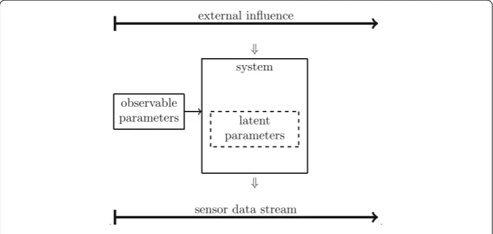
To model changes in the system, the parameters of the system are split into observable and latent parameters, see Fig.1. The observable parameters are inputs to the system and therefore the values of these parameters are known. Latent parameters describe external influences on the system (e.g., damage, fatigue, erosion). The values of the latent para-meters are unknown, except for the nominal latent parapara-meters that describe the nominal state of the system (e.g., no-damage condition). Since the values of the latent parameters are unknown, a reduced model can be built in the offline phase for the nominal latent parameter only. If the latent parameters change online (e.g., the system gets damaged), the reduced model fails to predict the behavior of the system. Rebuilding the reduced

system

⇓

⇓

latent parameters external influence

sensor data stream observable

parameters

model from scratch requires inferring the value of the changed latent parameters from the sensor data with a model of the changed system, then assembling the full model oper-ators corresponding to the inferred latent parameters, and deriving the reduced model. Rebuilding from scratch therefore is often too expensive in the context of online capabil-ity estimation, see, e.g., [1,33,37,42] for a discussion. The dynamic data-driven approach introduced in [42] exploits the sensor data of the system to adapt the reduced model to changes in the latent parameters online, without the computationally expensive inference step and without assembling the full model operators for the inferred latent parameters, see Fig.2.

There are several online adaptation approaches for reduced models. We distinguish between approaches that solely rely on pre-computed quantities for the adaptation and approaches that adapt the reduced model from new data that are generated during the online phase. Interpolation between reduced operators and reduced models [2,18,39,51], localization approaches [3,9,11,19–21,36,40,46], and dictionary approaches [30,35] rely on pre-computed quantities but do not incorporate information from new data into the reduced model online. In [4], local reduced models are adapted from partial data online to smooth the transition between the local models. In [12], anh-adaptive refinement is presented that splits basis vectors based on an unsupervised learning algorithm and residuals that become available online. The online adaptive approach [43] adapts the approximation of nonlinear terms from sparse data of the full model. There is also a body of work that rebuilds reduced models from scratch, e.g., in optimization [27,32,50], inverse problems [17,25], and multiscale methods [38]. We also mention that reduced models have been used in the context of dynamical data-driven application systems (DDDAS), which dynamically incorporate data into an executing application, and, in reverse, dynamically steer the measurement process. In [26], proper generalized decomposition [16] is used in a DDDAS to recover from device malfunctions by reconfiguring the simulation process. In [28], online parameter identification from measurements is considered for DDDAS with proper generalized decomposition. The work [1,33,34,37] considers model reduction for structural health monitoring in DDDAS.

Our extension to handle incomplete sensor samples in the dynamic data-driven reduced model adaptation builds on gappy proper orthogonal decomposition (POD), which is a

sensor data stream

initial latent parameters

assemble

full model

project

reduced model

read

adapt

dynamic reduced model

read

adapt

dynamic

reduced model . . .

method to approximate unknown or missing values in vector-valued data [22]. Gappy POD reconstructs the unknown values by representing the data vector as a linear combination of POD basis vectors. Applications of gappy POD in model reduction include flow field reconstruction [10,49], acceleration of efficient approximations of nonlinear terms [5,13,

24], and forecasting for time-dependent problems [14]. In our adaptation approach, we first construct a gappy POD basis from incomplete sensor samples using an incremental POD basis generation algorithm. The missing values of the incomplete sensor samples are then approximated in the space spanned by the obtained gappy POD basis. These approximate sensor samples are used in the dynamic data-driven adaptation to derive updates to the reduced model.

This paper is organized as follows. “Preliminaries and adaptation from complete data” section introduces the full model and the dynamic data-driven adaptation. “Incomplete sensor samples” section defines incomplete sensor samples and describes the problem setup in detail. “Dynamic data-driven adaptation from incomplete sensor samples” section introduces the extension to the dynamic data-driven adaptation approach that handles incomplete sensor samples. The numerical results in “Numerical results” section demon-strate that in our examples 30–40 % of the values of the sensor samples are sufficient to recover reduced models that accurately capture the changes in the latent parameters. “Summary and future work” section gives concluding remarks.

Preliminaries and adaptation from complete data

This section briefly discusses model reduction for systems with observable and latent parameters and summarizes the dynamic data-driven adaptation approach presented in [42].

Systems with latent parameters

Consider a parametrized system of equations stemming from the discretization of a para-metrized PDE

Aη(μ)y_η(μ)=f(μ). (1)

The full model (1) depends on the observable parameterμ ∈ D, whereD ⊂ Rd with d ∈N, and on the latent parameterη∈ E, whereE ⊂ Rd withd ∈ N. In general, the value of the latent parameter is unknown, only the value of a nominal latent parameter η0 ∈ E is known, see “Background” section. The linear operatorAη(μ) ∈ RN×N is an

N ×N matrix, where N ∈ Nis the number of degrees of freedom of the full model

(1). The linear operatorA_η(μ) depends on the observable and on the latent parameter. The operatorA_η(μ) has an affine parameter dependence with respect to the observable parameter

Aη(μ)=

lA

i=1 (i)

A(μ)A(ηi),

wherelA∈Nand(1)_A,. . .,(_AlA) :D→R. The linear operatorsA(1)_η ,. . .,A_η(lA)∈RN×N

f(μ)∈ RN _{depends on the observable parameter but is independent of the latent}

para-meter. The right-hand side has an affine parameter dependence with respect toμ

f(μ)=

lf

i=1 (i)

f (μ)f(i),

with_lf ∈N,(1)_{f ,}. . ._,(_flf):D→R, and theμ-independent vectorsf(1)_,. . ._,f(lf)∈RN_. Classical model reduction for systems with latent parameters

LetY_η0 ∈ RN×Mbe the snapshot matrix that contains as columnsM∈ Nstate vectors y_η0(μ₁),. . .,y_η0(μ_M) ∈ RN of the full model (1) corresponding to the observable para-metersμ1,. . .,μM ∈Dand the nominal latent parameterη0∈E. The POD basis matrix Vη0 ∈ RN×n contains as columns the firstn ∈ Nleft-singular vectors of the snapshot

matrixY_η0that correspond to the largest singular values. The POD basis vectors, i.e., the columns of the POD basis matrixV_η0, span then-dimensional POD spaceV_η0.

The reduced linear operator ˜A_η0(μ)∈Rn×n_{is obtained via Galerkin projection of the}

equations of the full model onto the POD spaceV_η0. Consider therefore the projected μ-independent operators

˜

A(_ηi₀)=VT η0A

(i)

η0Vη0, i=1,. . ., lA.

By exploiting the affine parameter dependence of the linear operatorA_η0(μ) on the observ-able parameterμ∈D, the reduced linear operator ˜A_η0(μ) is

˜ Aη0(μ)=

lA

i=1 (i)

A(μ) ˜A (i) η0.

Similarly, the reduced right-hand side is

˜ f_η0(μ)=

lf

i=1 (i)

f (μ)˜f (i)

,

where ˜f(i)=VT_η0f(i)∈Rnfori=1,. . ., lf. The reduced model for the latent parameter

η0is

˜

Aη0(μ)˜yη0(μ)=

˜

f_η0(μ), (2)

where ˜y_η

0(μ)∈R

n_{is the reduced state. The reduced right-hand side ˜f}

η0(μ)∈R n_{in the}

reduced model (2) depends on the latent parameterη₀because of the projection onto the POD spaceV_η0, in contrast to the right-hand side vectorf(μ)∈RN in the full model (1). Dynamic data-driven adaptation for reduced models

latent parameterη₀to the changed latent parameter, say,η₁∈E_.1_{In each adaptivity steph,}

a sensor sample ˆy_η1(μ_M+h)∈RNis received. The sensor sample ˆy_η1(μ_M+h) is an approx-imation of the statey_η1(μ_M+h) for the changed latent parameterη₁and an observable

parameterμ_M+h ∈ D. The differenceyˆ_η1μ_M+h−y_η1μ_M+hbetween the sensor sample and the state in a norm · is noise, measurement error, and the discrepancy of the full model and reality (model discrepancy [31]). At steph, the sensor samples matrix Sh ∈ RN×h contains the received sensor samples ˆyη1(μM+1),. . .,yˆη1(μM+h) ∈ R

N _as

columns

Sh=

ˆ

y_η1μM+1

,. . .,yˆ_η

1

μM+h

∈RN×h_.

At each adaptivity steph=1,. . ., M, the dynamic data-driven adaptation first adapts the POD basis and then the reduced operators. Consider the POD basis adaptation first. At steph = 1, the first snapshot, i.e., the first column, in the snapshot matrixY_η0 is replaced with the sensor sample ˆy_η

1(μM+1)∈R

N _{and the snapshot matrix at steph=1}

is obtained

Y1=

ˆ

y_η1μM+1

,y_η0(μ2),. . .,yη0(μM)

∈RN×M_.

Note that there is no particular ordering of the snapshots in the snapshots matrix. We replace the first column ofY_η0 because we are at steph=1. By reordering the columns ofY_η0, any other snapshot can be replaced at steph= 1. The matrixY1is the result of an additive rank-one update to the snapshot matrixY_η0. Lete_i∈ {0,1}Nbe the canonical unit vector with 1 at componentiand 0 at all other components fori=1,. . ., N. Then, the snapshot matrixY1is

Y1=Yη0+aeT1,

where a = yˆ_η1(μ_M+1)−y_η0(μ1) ∈ RN. Therefore, the POD basis matrixV1 ∈ RN×n corresponding to the snapshot matrixY1can be approximately derived fromVη0via the

adaptation algorithm [8]. The algorithm extracts the componentsα=a−V_η0VT_η

0aand

β=e1−Vη0VTη0e1ofaande1, respectively, that are orthogonal toVη0. The vectorsαand

βare used to derive a rotation matrixV∈Rn×nof sizen×nand an additive rank-one updateγδT withγ ∈ RN andδ∈ Rn. Computing the rotation matrix and the rank-one update requires computing the singular value decomposition (SVD) of an (n+1)×(n+1) matrix. The adapted POD basis matrixV1is then given by

V1=Vη0V+γδ T_.

Note that an SVD of a typically small (n+1)×(n+1) matrix is required by the adaptation algorithm, instead of the SVD of anN×Mmatrix if the POD basis matrix were computed directly fromY1without reusingVη0. We refer to [8] for details on the adaptation of the

POD basis matrix. The adaptation algorithm is summarized in [42, Algorithm 1] for the case of the dynamic data-driven adaptation.

Consider now the adaptation of the operators at steph=1. The goal is to approximate the reduced operators

˜

A(_ηi₁)=VT

1A(ηi1)V1, i=1,. . ., lA,

1_{Note that the adaptation can be repeated to adapt fromη}

without assembling the full operators A(1)_η

1,. . .,A

(lA)

η1 ∈ R

N×N _{corresponding to the}

changed latent parameterη₁. Therefore, at adaptivity steph=1, the operators ¯

A(i)

1 =VT1A(ηi0)V1, i=1,. . ., lA, (3)

are constructed. The operator ¯A(₁i)is the full operatorA(_ηi)

0for latent parameterη0projected

onto the adapted POD spaceV1with the adapted POD basis matrixV1, fori=1,. . ., lA.

Note that (3) projects the full operators corresponding to the nominal latent parameterη₀, and not the operators corresponding to the changed latent parameterη₁. Then, additive updatesδA˜(1)₁ ,. . .,δA˜1(lA) ∈Rn×nare derived from the sensor sample matrixS1with the optimization problem

min δ_A˜(1)_{h ,...,δA}˜(lA)

h ∈Rn×n h j=1 lA i=1 (i)

A(μM+j)

¯

A(_hi)+δ_A˜(i)

h VThˆyη1(μM+j)−

˜

fh(μM+j)

2 2 , (4)

where ˜f_h(μ_M+j)∈Rnis the reduced right-hand side with respect to the POD basisV_h. Note that the optimization problem (4) is formulated for generalh≥1, and not only for h=1. The solution of the optimization problem (4) are the updatesδA˜(1)_h ,. . .,δA˜(_hlA)that best-fit the sensor samples in the sensor sample matrixS_h. The optimization problem (4) is a least-squares problem that can be solved with, e.g., the QR decomposition. Forh< lAn, the least-squares problem is underdetermined, and only low-rank approximations of δ_A˜(1)

h ,. . .,δA˜ (lA)

h are computed [42].

At steph=1, the adapted operators are ˜

A(1i)=A¯ (i) η0+δA˜

(i)

1, i=1,. . ., lA,

and the adapted reduced operator ˜A1(μ)∈Rn×ncan be assembled using the affine para-meter dependence as

˜ A1(μ)=

lA

i=1 (i)

lA(μ) ˜A (i) 1.

In each adaptivity step h = 1,. . ., M, this POD basis and operator adaptation is repeated. This means, at steph, the POD basis matrix is adapted fromV_h−1toVhby

exploiting that the snapshot matrixY_hat stephis the result of a rank-one update to the snapshot matrixY_h−1from the previous step. The adapted reduced operator ˜A_h(μ) is

derived via the additive rank-one updatesδA˜(1)_h ,. . .,δA˜(_hlA) ∈ Rn×n, which are obtained via optimization from the sensor samples matrixS_h=

ˆ

y_η1μM+1

,. . .,ˆy_η1μ_M+h∈ RN×h_{. For sufficiently many sensor samples, and if the sensor samples are noise-free, the}

reduced operator ˜A_η1(μ) with respect to the POD basis matrixV_hequals the adapted reduced operator ˜A_h(μ), see [42].

Incomplete sensor samples

Let ˆy_η

1(μM+h)∈R

N_{be the (complete) sensor sample that is received at adaptivity step}

h. Letk ∈ Nwithk < N and letp1h,. . ., phk ∈ {1,. . ., N}be pairwise distinct indices of

the sensor sample ˆy_η1(μ_M+h)∈ RN. The indicesp1h,. . ., phk give rise to a point selection

matrix

Ph=

e_ph

1,. . .,ephk

∈RN×k_.

The point selection matrixP_hselects the components with indicesph1,. . ., phk. For example,

consider the vectorx=[x1,. . ., xN]T ∈RN, then we have

⎡ ⎢ ⎢ ⎣

x_ph

1

.. . x_ph

k

⎤ ⎥ ⎥ ⎦=PThx.

From the point selection matrixP_h, we derive the matrixQ_h∈RN×(N−k)that selects the components of the (complete) sensor sample ˆy_η

1(μM+h) that are missing in the incomplete

sensor sample ˆyincp_η1 (μ_M+h). The matricesP_handQ_hlead to the decomposition

ˆ

y_η1(μ_M+h)=P_hPT_hyˆ_η1(μ_M+h)+Q_hQT_hyˆ_η1(μ_M+h).

The matrixP_hPT_h selects all components that correspond to the indicesp1h,. . ., phkand sets

the components at all other indices{1,. . ., N} \

ph1,. . ., phk

to zero. The matrixQ_hQT_h

has the opposite effect and selects all components with indices in{1,. . ., N}\

ph1,. . ., phk

and sets the components with indices

ph1,. . ., phk

to zero.

We define the incomplete sensor sample ˆyincp_η1 (μ_M+h) of the (complete) sensor sample ˆ

y_η1(μ_M+h) corresponding to the point selection matrixP_has

ˆ yincp

η1 (μM+h)=PhP

T

hyˆη1(μM+h)∈R

N_{. (5)}

The values at the components of the incomplete sensor sample ˆyincp_η1 (μ_M+h) with indices ph1,. . ., phk are set to the corresponding components of the (complete) sensor sample

ˆ

y_η1(μ_M+h). All other components are missing in the incomplete sensor sample and their values in ˆyincp_η1 (μ_M+h) are zero through the definition (5).

Dynamic data-driven adaptation from incomplete sensor samples

We propose an extension to the dynamic data-driven adaptation approach that handles incomplete sensor samples. Consider the adaptation from the nominal latent parameter η0to the latent parameterη1in theMadaptivity stepsh=1,. . ., M. At each adaptivity step h = 1,. . ., M, we receive incomplete sensor samples ˆy_ηincp₁ (μ_M+h) ∈ RN and the corresponding point selection matricesP_h. The point selection matrix depends onhand might change at each adaptivity step, see the discussion on future sensor technologies in “Background” section. The number of known componentskis independent ofhand stays constant for allh=1,. . ., M.

We split the adaptivity stepsM =Mbasis+MupdateintoMbasis∈NandMupdate ∈N steps. In the firsth=1,. . ., Mbasissteps, a gappy POD basis is derived from the incom-plete sensor samples ˆyincp_η1 (μ_M+1),. . .,yˆincp_η1 (μ_M+Mbasis)∈RN. At the subsequentMupdate

stepsh= M+Mbasis+1,. . ., M, the missing values of the incomplete sensor samples ˆ

y_η1μ_M+Mbasis_+h

basis. The approximations of the missing values and the components in the incomplete sensor sample are combined to approximate the complete sensor sample. The dynamic data-driven adaptation is then applied to these approximate sensor samples to update the reduced model. “Deriving the gappy POD basis” section discusses the construction of the gappy POD basis and “Dynamic data-driven adaptation from approximate sensor samples” section presents the adaptation of the reduced model from the approximate sen-sor samples. “Computational procedure” section summarizes the procedure and presents Algorithm 1.

Deriving the gappy POD basis

In the first h = 1,. . ., Mbasis adaptivity steps, we derive a gappy POD basis from the

incomplete sensor samples. Letr ∈ Nbe the dimension of the gappy POD basis with

gappy POD basis matrixU_h ∈ RN×r. The initial gappy POD basis matrixU0 ∈ RN×r contains as columns ther-dimensional POD basis vectors corresponding to the snapshot matrixY_η0.

At step h = 1, we receive the incomplete sensor sample ˆyincp_η1 (μ_M+1) and the corre-sponding point selection matrixP1 ∈ RN×k with Q1 ∈ RN×(N−k). We use the initial gappy POD basis matrixU0to derive the approximate sensor sample ˆyapprxη1 (μM+1)∈R

N

using gappy POD [10,22,49]

ˆ yapprx

η1 (μM+1)=Q1Q

T 1U0

PT

1U0 +

PT 1yˆ

incp η1

μM+1

+yˆincp_η1 μ_M+1. (6) The matrix (PT₁U0)+∈Rr×kis the Moore–Penrose pseudoinverse of the matrixPT1U0∈ Rk×r_{. SinceP}T

1yˆ incp

η1 (μM+1)=P

T

1yˆη1(μM+1), we have that (P T

1U0)+PT1yˆ incp

η1 (μM+1) is the

solution of the regression problem

arg min

c∈Rr

PT

1

U0c−yˆ_η1

μM+1 2

2. (7)

Note that the regression problem is overdetermined and has a unique solution if the matrix PT

1U0has full column rank, which we typically ensure by selectingk>r. Therefore, the vectorU0

PT

1U0

+_PT 1yˆ

incp

η1 (μM+1)∈ RN is the best approximation with respect to (7)

of the complete sensor sample ˆy_η

1(μM+1) in the space spanned by the columns of the

POD basis matrixU0. The approximate sensor sample ˆyapprxη1 (μM+1) combines this best

approximation and the known values in the incomplete sensor sample. The values at the components corresponding to the missing components of the incomplete sensor sample are set to the best approximation, and the values at all other components are set to the values obtained from the incomplete sensor sample.

We then use the approximate sensor sample ˆyapprx_η1 (μ_M+1) to adapt the gappy POD basis fromU0toU1. Consider therefore the snapshot matrixY0and note thatU0is thek -dimensional POD basis derived fromY0. We adapt the snapshot matrixY0toY1∈RN×M via a rank-one update that replaces column 1 ofY0with the approximate sensor sample ˆ

yapprx

η1 (μM+1)∈RN. SinceY1is the result of a rank-one update toY0, thek-dimensional

At step _h = 2, the approximate sensor sample ˆyapprx_η1 (μ_M+2) is constructed with the gappy POD basis matrixU1, which is then used to adapt fromU1toU2. This process is continued until steph=Mbasis, where the gappy POD basis matrixU_Mbasisis derived.

Note that the number of columns in the snapshot matrix is fixed and that columns are replaced following the first-in-first-out principle ifh>M.

Dynamic data-driven adaptation from approximate sensor samples

In theMupdatestepsh=M+Mbasis+1,. . ., M, we adapt the reduced model from approx-imate sensor samples using the dynamic data-driven adaptation. Consider therefore an adaptivity steph>Mbasis_{, at which the incomplete sensor sample ˆy}incp

η1 (μM+h)∈RN and

the corresponding point selection matrixP_h∈Rk×Nare received. We use the gappy POD basisU_Mbasisto derive the approximate sensor sample ˆyapprxη₁ (μ_M+h) of the complete sensor

sample with the gappy POD basisU_Mbasis. The approximate sensor sample ˆyapprxη₁ (μ_M+h)

is then used to adapt the reduced model with the dynamic data-driven adaptation as described in “Dynamic data-driven adaptation for reduced models” section.

Computational procedure

Algorithm 1 summarizes the dynamic data-driven adaptation that can handle incomplete sensor samples. Inputs of Algorithm 1 are the POD basis matrix V_h−1, the operators

˜

A(1)_h−1,. . .,A˜(hl−1A), and the right-hand sides ˜f (1) h−1,. . .,f˜

(lf)

h−1derived at the previous adaptivity steph−1. Ifh≤Mbasis, the algorithm adapts the gappy POD basis fromU_h−1toU_husing the approach presented in“Deriving the gappy POD basis” section. First, the approximate

sensor sample is constructed with gappy POD. Then, the adapted basis matrix U_h is

computed with the incremental POD algorithm [8]. Only the gappy POD basis is adapted and the reduced model is returned unchanged. If h > Mbasis, the approximate sensor sample is derived with gappy POD andU_Mbasis. The approximate sensor sample is then

used with the dynamic data-driven adaptation to derive the adapted POD basisV_h, the adapted operators ˜A(1)_h ,. . .,A˜(_hlA),and the adapted right-hand sides ˜f(1)_h ,. . .,f˜(_hlf).

Algorithm 1 Dynamic data-driven adaptation from incomplete sensor samples

1: procedureadaptIncomplete(Mbasis,Uh−1,Vh−1,A˜(1)h−1, . . . ,A˜(hl−1A),f˜h(1)−1, . . . ,f˜ (lf)

h−1) 2: Receive incomplete sensor sampleyˆ_ηincp₁(µ_M+h)∈RN and point selection matrixP_h∈Rk×N 3: Construct matrixQ_h∈R(N−k)×N

4: ifh≤Mbasis_then

5: Compute approximate sensor sample using gappy POD basis matrixU_h−1

ˆ yapprx

η1 (µM+h) =QhQ T

hUh−1(PhTUh−1)+PhTyˆincpη1 (µM+h) + ˆy

incp η1(µM+h).

6: Update snapshot matrix_Yh−1with_yˆηapprx

1 (µM+h)to obtainYh 7: Derive adapted gappy POD basis matrix_Uhfrom_Uh−1using [8]

8: Set_A˜(_hi)_{= ˜Ah}(i₋₁) for_{i= 1, . . . , lA}

9: Set_f˜_h(i)_{= ˜fh}(i₋₁) for_{i= 1, . . . , lf}

10: SetV_h=V_h−1 11: else

12: Compute approximate sensor sample using basisU_Mbasis

ˆ yapprx

η1 (µM+h) =QhQ T

hUMbasis(P_hTU_Mbasis)+P_hTyˆ_ηincp

1(µM+h) + ˆy

incp η1(µM+h).

13: GetV_h,A˜_h(1), . . . ,A˜(_hlA),f˜_h(1), . . . ,f˜_h(lf)from dynamic adaptation withyˆ_ηapprx

1 (µM+h) 14: end if

Numerical results

This section demonstrates the dynamic data-driven adaptation from incomplete sensor samples on a model of a bending plate. The latent parameter describes damage of the plate. The damage is a local decrease of the thickness of the plate. The model is based on the Mindlin plate theory [23,47] that takes into account transverse shear deformations but neglects important nonlinear effects such as postbuckling behavior. Therefore, the model that we use in this section is a simple description of a plate in bending. We use the plate model only to provide a proof of concept of our adaptation approach. More advanced plate models are used in real-world engineering applications. We refer to “Summary and future work” section for a discussion on further applications of our adaptation approach. We first build a reduced model for the nominal problem, i.e., the latent parameter is set to the nominal latent parameterη₀ ∈ Dthat corresponds to the no-damage condition. We then decrease the thickness of the plate stepwise and adapt the reduced model. After each change in the latent parameter, synthetic incomplete sensor samples are computed with the full model, which are used to adapt the reduced model. The following sections give details on the problem setup and report the numerical results.

Plate problem

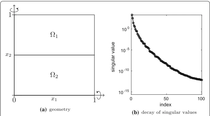
We consider the static analysis of a plate in bending. The plate is clamped into a frame and a load is applied. Our problem is an extension of the plate problems introduced in [23,42,44]. The geometry of our plate problem is shown in Fig.3a. The spatial domain∈ [0,1]2⊂R2is split into two subdomains=1∪2. The problem has three observable parameters μ = [μ1,μ2,μ3]T ∈ D with D = [0.05,0.1]2×[1,100]. The observable parametersμ1andμ2control the nominal thickness of the plate in the subdomain1 and2, respectively. The third observable parameterμ3defines the load on the plate.

The latent parameterη=[η1,η2]T ∈Econtrols the damage of the plate, i.e., the latent parameter defines the local decrease of the thickness that corresponds to the damage. The

Ω

Ω

x1

x2

1

0

1

0 50 100

index 10-15

10-10 10-5 100

singular value

decay of singular values

(b)

geometry

(a)

domain of the latent parameter isE = [0_,0_.2]×(0_,0_.05]. The thickness of the plate at positionx∈is given by the functiont:×D×E→Rwith

t(x;μ,η)=t0(x;μ)

1−η1exp

− 1

2η2₂x−z 2 2

,

and

t0(x;μ)= ⎧ ⎨ ⎩

μ1 ifx1>0.5 μ2 ifx1≤0.5 ,

with positionz = [0.7,0.4]T ∈ . The functiontis nonlinear inx,μandη. We set the nominal latent parameterη₀toη₀=[0,0.01]T ∈Ethat corresponds to no local decrease of the thickness and therefore to the no-damage condition.

The full model of the plate problem is a finite element model, see [23]. The corresponding system of equations is of the form (1), wherelA=4,lf =1,(1)f (μ)=μ3,

(1)

A (μ)=μ31, (2)

A (μ)=μ32,

and

(3)

A (μ)=μ1, (4)

A (μ)=μ2

The system of equations hasN =4719 degrees of freedom. The thickness of the plate with μ = [0.08,0.07,50]T _{∈ Dand withη= η}

0is visualized in Fig.4a and the deflection in

spatial coordinatex1 spatial coordinatex1

spatial coordinatex1

spatial coordinatex1

spatial coordinate x2 spatial coordinate x2 spatial coordinate x2 spatial coordinate x2

0 0.2 0.4 0.6 0.8 1

1 0.8 0.6 0.4 0.2 0 thickness 0.05 0.06 0.07 0.08

0 0.2 0.4 0.6 0.8 1

1 0.8 0.6 0.4 0.2 0 thickness 0.05 0.06 0.07 0.08

thickness, damage up to 20% (b)

thickness, no damage (a)

0 0.5 1

0 0.2 0.4 0.6 0.8 1 deflection -0.6 -0.5 -0.4 -0.3 -0.2 -0.1 0

0 0.5 1

0 0.2 0.4 0.6 0.8 1 deflection -0.6 -0.5 -0.4 -0.3 -0.2 -0.1 0

deflection, damage up to 20% (d)

deflection, no damage (c)

Fig.4c. The thickness and the deflection of the plate with a damage up to 20 %, i.e., a local decrease of the thickness of the plate atzby 20 %, is shown in Fig.4b and d, respectively. We drawM=1000 observable parametersμ1,. . .,μM ∈Duniformly inDand

com-pute the corresponding state vectors with the full model to assemble the snapshot matrix

Yη0 =

ˆ

y_η0(μ₁),. . .,yˆ_η

0(μM)

∈RN×M_.

Note that the latent parameterη=η₀is set to the nominal latent parameterη₀. Figure3b plots the decay of the singular values of the snapshot matrixY_η0. We construct a reduced model via Galerkin projection onto the space spanned by the firstn=8 POD basis vectors ofY_η0.

Setup of numerical experiments

We now describe the details of our numerical experiments. We have ten latent parameters η0,η1,. . .,η9 ∈ E, whereη0is the nominal latent parameter corresponding to the no-damage condition and

ηi=

2i 90,

2i 360

T

∈E, i=1,. . .,9.

This means that from latent parameterη_i−1toη_ithe thickness at positionzis decreased by a factor of two, fori= 1,. . .,9. After each change of the latent parameter, the sensor

window is flushed and M ∈ Nincomplete sensor samples are received to adapt the

reduced model.

Number of sensor samples

We receive incomplete sensor samples, and therefore we use the extension to the dynamic data-driven adaptation described in “Dynamic data-driven adaptation from incomplete sensor samples” section. This means that the adaptivity steps h = 1,. . ., M required for adapting from latent parameterη_i−1toη_i are split intoMbasis ∈ Nsteps to derive

the gappy POD basis andMupdate _{∈ Nsteps to update the reduced model. We chose}

Mbasis_andMupdate_{conservatively in the following, because we are primarily interested in} studying the effect of the number of missing components in the incomplete sensor samples onto the adaptation, rather than the number of sensor samples; see [42] for studies on the effect of the number of samples on the dynamic data-driven adaptation in the case with complete sensor samples. We setMbasis=5000 and therefore derive the gappy POD basis fromMbasis=5000 incomplete sensor samples. We buffer 50 incomplete sensor samples and use them in the incremental basis generation procedure described in “Deriving the gappy POD basis” section.

The theory of the dynamic data-driven adaptation with complete sensor samples gives guidance on the selection ofMupdate_{. In case of complete sensor samples, settingM}update₌ lA×nis sufficient to recover the reduced model that would be obtained via rebuilding

from scratch [42]. Note thatlA=4 is the number ofμ-independent operators andn=8

the dimension of the POD basis space. We setMupdate = 5×lA×n = 160 since we

Sensor sample generation

The number of missing componentsN−kin the incomplete sensor samples is controlled by the number of known componentsk. To discuss the effect ofkon the adaptation, we introduce separate numbers of known componentskbasis ∈ Nandkupdate ∈ Nfor the gappy POD basis construction and the update, respectively. Furthermore, we introduce the sensor rates

ρbasis₌ kbasis

N ×100, ρ

update₌ kupdate N ×100,

which are the percent of the number of known components of the total number of com-ponents_N in the incomplete sensor samples. Thus, for example,ρbasis _{= 100 % means} that all components are known and therefore that we have a complete sensor sample.

We synthetically generate incomplete sensor samples with the full model at each step h = 1,. . ., M. We therefore first draw uniformly an observable parameter μ_M+h in

D and compute the state vector y_η(μ_M+h) with the full model for the current latent parameterμ. We then drawk∈Nunique indices uniformly in{1,. . ., N}and construct the point selection matrixP_h ∈RN×k. The incomplete sensor sample is ˆyincp_η (μ_M+h)= PhPT_hyη(μM+h).

Error computation

We compare three reduced models:

• A static reduced model that is built as described in “Classical model reduction for systems with latent parameters” section. The static reduced model is not adapted to changes in the latent parameter.

• A rebuilt reduced model that is derived as in “Classical model reduction for sys-tems with latent parameters” section but from Mupdate complete sensor samples corresponding to the current changed latent parameter. This requires repeating the computation of the POD basis and the operator projections, which is prohibitively expensive to conduct online.

• An online adaptive reduced model that is adapted to changes in the latent parameter from incomplete sensor samples with the dynamic data-driven adaptation described in Algorithm 1.

To assess the quality of the reduced models quantitatively, we draw ten observable para-metersμ₁,. . .,μ10∈Duniformly inDand compute the relativeL2error with respect to the full model

er=

1 10

10

i=1

¯y_η(μ_i)−y_η(μ_i) 2

y_η(μ_i)

2

, (8)

whereηis the current latent parameter and ¯y_η(μ₁),. . .,y¯_η(μ₁₀)∈Rn_{are the state vectors}

obtained with either the static, the rebuilt, or the adapted reduced model.

Gappy POD basis from complete sensor samples

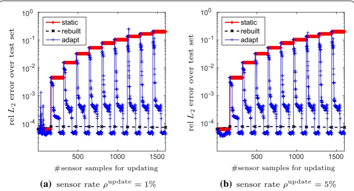
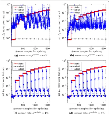
Figures5and6demonstrate the effect of the sensor rateρupdate_{on the dynamic} data-driven adaptation. First consider the static reduced model. As the latent parameter changes fromη₀(no damage) toη₉(20 % decrease of thickness), the error of the static reduced model increases by three orders of magnitude. The steps in the error curve reflect the changes in the latent parameter. The error of the rebuilt reduced model stays near 10−4. Consider now the adaptive reduced model. The dimension of the gappy POD basis is set to r = 30. Figure 5shows that a sensor rate ρupdate = 0.6 % leads to an adapted reduced model with large errors. A sensor rate ofρupdate=0.6 % means thatkupdate=29 components of the incomplete sensor sample are known, and thereforekupdate_{<r. This} violates the condition of gappy POD that requires a full-column rank PT_hU_Mbasis, see

“Deriving the gappy POD basis” section. For a slightly larger sensor rateρupdate_{=0.8 %,} andkupdate > r, our dynamic data-driven adaptation from incomplete sensor samples recovers the rebuilt reduced model. Figure 6 indicates that increasing the sensor rate

ρupdate _{reduces the error of the adapted reduced model in the first few adaptivity steps} after a change in the latent parameter, cf. Fig.5.

Note that the adapted reduced model achieves a slightly lower error than the rebuilt

reduced model in Figs. 5 and 6. The dynamic data-driven adaptation constructs the

adapted operators with an optimization problem from the sensor samples projected onto the POD space. This projection and the optimization cause the difference in the error of the adapted and the rebuilt reduced model, if the dimension of the reduced model is low. The difference decreases if the dimension of the reduced model is increased, see [42, Theorem 1].

500 1000 1500

# sensor samples for updating # sensor samples for updating

10-4

10-3

10-2

10-1

100

rel

L2

error over test set

rel

L2

error over test set

static rebuilt adapt

500 1000 1500

10-4

10-3

10-2

10-1

100

static rebuilt adapt

(a) sensor rateρupdate= 0.6% (b) sensor rateρupdate= 0.8%

500 1000 1500

#sensor samples for updating #sensor samples for updating

10-4 10-3 10-2 10-1 100

rel

L2

error over test set

rel

L2

error over test set

static rebuilt adapt

500 1000 1500 10-4

10-3 10-2 10-1 100

static rebuilt adapt

(a) sensor rateρupdate=1% (b) sensor rateρupdate= 5%

Fig. 6 The gappy POD basis is derived from complete sensor samples (i.e.,ρbasis_{=100 %) but the sensor} rate for the incomplete sensor samples received during theMupdate_{update steps is set toρ}update_{=1 % (a)} andρupdate_{=5 % (b). The dimension of the gappy POD basis is set tor=30}

Figure7reports the error behavior of an adapted reduced model that uses a gappy POD basis of dimensionr=40. Forρupdate _{=0.6 % andρ}update _{=0.8 %, we again obtain the} situationkupdate<rand therefore obtain an underdetermined least-squares problem that introduces large errors in the adaptation. However, if the sensor rateρupdateis increased, the approximation quality of the adapted reduced model increases too. The results in Fig.6forr=30 are similar to the result obtained in Fig.7forr=40. This shows that a gappy POD basis withr=30 dimensions is sufficient in this example.

Gappy POD basis from incomplete sensor samples

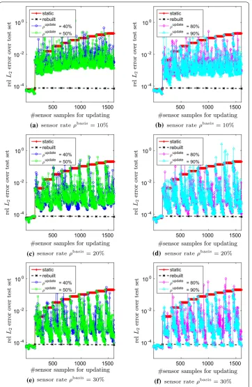
We now consider the situation whereρbasis_{<100 % andρ}update_{<100 %, i.e., the gappy} POD basis is derived from incomplete sensor samples and the updates to the reduced models are obtained from incomplete sensor samples as well. Figure8shows the effect of the sensor rateρbasison the adaptation. Figures8a and b demonstrate that a sensor rate

ρbasis _{=10 % is too low to recover the rebuilt reduced model with the adapted reduced} model in this example. Even setting the sensor rate for the update toρupdate = 90 % (i.e., generating the gappy POD basis from incomplete samples withρbasis = 10 % and

updating the reduced model from approximate sensor samples with ρupdate = 90 %)

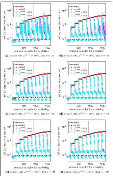
cannot compensate the inadequate sensor rateρbasis= 10 %. Increasing the sensor rate for the gappy POD basis construction toρbasis=30 % leads to an adapted reduced model that recovers the rebuilt reduced model. However, withρbasis_{=30 % there still are outliers} that lead to a reduced model with a large error. Figure9shows that increasing the sensor rate toρbasis=70 % reduces those outliers significantly. Again, increasing the dimension of the gappy POD basis from r = 30 tor = 40 only slightly reduces the error of the adapted reduced model, compare Fig.9a, c, e with Fig.9b, d, f.

(a) (b)

(c) (d)

Fig. 7 Increasing the dimension of the reconstruction basis tor=40 only slightly decreases the error of the adapted reduced model, compared to a reconstruction basis withr=30 (see Figs.5,6). Note that

ρupdate_{>0.8 % is required to obtain an overdetermined regression problem in gappy POD in this example}

(a) (b)

(c) (d)

(e) (f)

(a) (b)

(d) (c)

(e) (f)

(a) (b)

Fig. 10 This figure compares the runtime of the dynamic data-driven adaptation to rebuilding the reduced model from scratch. Adapting the reduced model using our approach is about two orders of magnitude faster than rebuilding the reduced model from scratch

Summary and future work

We proposed an extension to the dynamic data-driven adaptation that handles incom-plete sensor samples, i.e., partial measurements of the large-scale state. In our approach, a gappy POD basis is derived from incomplete sensor samples. The missing values of the incomplete sensor samples are approximated with gappy POD in the space spanned by the gappy POD basis. The reduced model is then adapted using the gappy POD approx-imations of the complete sensor samples with the dynamic data-driven adaptation. The numerical results confirm that about 30–40 % of the total number of components of the sensor samples are sufficient to recover the reduced model that would be obtained via rebuilding from scratch.

Future sensing technologies (e.g., “sensor skins”) of next-generation engineering sys-tems will provide high-resolution measurements. Processing these large data sets will be computationally challenging. In big data analytics, sublinear algorithms are currently developed that look at only a subset of the given data set to meet runtime requirements [48]. Our approach follows a similar paradigm. We selectively process sensor data that are most informative for deriving the update to the reduced model and ignore large parts of the received data that are irrelevant in the current situation. Our approach is applicable even if the selection of the high-resolution sensor data is dynamically changing online, e.g., due to new damage events.

that have all components set to zero, and then adapt these operators to the available data. Such a system identification approach would derive a reduced model directly from data. In general, our approach is applicable to DDDAS for which massive amounts of sensor data are available.

Authors’ contributions

BP and KW developed the methodology, performed the numerical investigations, and wrote the manuscript. All authors read and approved the final manuscript.

Acknowledgements

This work was supported in part by the AFOSR MURI on multi-information sources of multi-physics systems under Award Number FA9550-15-1-0038, program manager Jean-Luc Cambier, and by the United States Department of Energy Applied Mathematics Program, Awards DE-FG02-08ER2585 and DE-SC0009297, as part of the DiaMonD Multifaceted Mathematics Integrated Capability Center. Some of the numerical examples were computed on the computer cluster of the Munich Centre of Advanced Computing.

Competing interests

The authors declare that they have no competing interests.

Received: 28 November 2015 Accepted: 8 March 2016

References

1. Allaire D, Chambers J, Cowlagi R, Kordonowy D, Lecerf M, Mainini L, Ulker F, Willcox K. An offline/online DDDAS capability for self-aware aerospace vehicles. Procedia Comput Sci. 2013;18:1959–68.

2. Amsallem D, Farhat C. An online method for interpolating linear parametric reduced-order models. SIAM J Sci Comput. 2011;33(5):2169–98.

3. Amsallem D, Zahr M, Farhat C. Nonlinear model order reduction based on local reduced-order bases. Int J Numer Methods Eng. 2012;92(10):891–916.

4. Amsallem D, Zahr M, Washabaugh K. Fast local reduced basis updates for the efficient reduction of nonlinear systems with hyper-reduction. Special issue on model reduction of parameterized systems (MoRePaS). Adv Comput Math. 2014. (accepted).

5. Astrid P, Weiland S, Willcox K, Backx T. Missing point estimation in models described by proper orthogonal decom-position. Autom Control IEEE Trans. 2008;53(10):2237–51.

6. Barrault M, Maday Y, Nguyen N, Patera A. An empirical interpolation method: application to efficient reduced-basis discretization of partial differential equations. Comptes Rendus Math. 2004;339(9):667–72.

7. Benner P, Gugercin S, Willcox K. A survey of projection-based model reduction methods for parametric dynamical systems. SIAM Rev. 2015;57(4):483–531.

8. Brand M. Fast low-rank modifications of the thin singular value decomposition. Linear Algebra Appl. 2006;415(1):20– 30.

9. Brunton SL, Tu JH, Bright I, Kutz JN. Compressive sensing and low-rank libraries for classification of bifurcation regimes in nonlinear dynamical systems. SIAM J Appl Dyn Syst. 2014;13(4):1716–32.

10. Bui-Thanh T, Damodaran M, Willcox K. Aerodynamic data reconstruction and inverse design using proper orthogonal decomposition. AIAA J. 2004;42(8):1505–16.

11. Burkardt J, Gunzburger M, Lee H-C. POD and CVT-based reduced-order modeling of Navier–Stokes flows. Comput Methods Appl Mech Eng. 2006;196(1–3):337–55.

12. Carlberg K. Adaptive h-refinement for reduced-order models. Int J Numer Methods Eng. 2015;102(5):1192–210. 13. Carlberg K, Bou-Mosleh C, Farhat C. Efficient non-linear model reduction via a least-squares petrov-galerkin projection

and compressive tensor approximations. Int J Numer Methods Eng. 2011;86(2):155–81.

14. Carlberg K, Ray J, van Bloemen Waanders B. Decreasing the temporal complexity for nonlinear, implicit reduced-order models by forecasting. Comput Methods Appl Mech Eng. 2015;289:79–103.

15. Chaturantabut S, Sorensen D. Nonlinear model reduction via discrete empirical interpolation. SIAM J Sci Comput. 2010;32(5):2737–64.

16. Chinesta F, Ladeveze P, Cueto E. A short review on model order reduction based on proper generalized decomposi-tion. Arch Comput Methods Eng. 2011;18(4):395–404.

17. Cui T, Marzouk YM, Willcox KE. Data-driven model reduction for the bayesian solution of inverse problems. Int J Numer Methods Eng. 2015;102(5):966–90.

18. Degroote J, Vierendeels J, Willcox K. Interpolation among reduced-order matrices to obtain parameterized models for design, optimization and probabilistic analysis. Int J Numer Methods Fluids. 2010;63(2):207–30.

19. Dihlmann M, Drohmann M, Haasdonk B. Model reduction of parametrized evolution problems using the reduced basis method with adaptive time-partitioning. In: Aubry D, Díez P, Tie B, Parés N, editors, Proceedings of the international conference on adaptive modeling and simulation; 2011. p. 156–67.

20. Eftang J, Patera A. Port reduction in parametrized component static condensation: approximation and a posteriori error estimation. Int J Numer Methods Eng. 2013;96(5):269–302.

21. Eftang J, Stamm B. Parameter multi-domain hp empirical interpolation. Int J Numer Methods Eng. 2012;90(4):412–28. 22. Everson R, Sirovich L. Karhunen–Loève procedure for gappy data. J Opt Soc Am A. 1995;12(8):1657–64.

24. Galbally D, Fidkowski K, Willcox K, Ghattas O. Non-linear model reduction for uncertainty quantification in large-scale inverse problems. Int J Numer Methods Eng. 2010;81(12):1581–608.

25. Garmatter D, Haasdonk B, Harrach B. A reduced landweber method for nonlinear inverse problems. Technical report, University of Stuttgart; 2015. Available at Arxiv.

26. Ghnatios C, Masson F, Huerta A, Leygue A, Cueto E, Chinesta F. Proper generalized decomposition based dynamic data-driven control of thermal processes. Comput Methods Appl Mech Eng. 2012;213–216:29–41.

27. Gogu C. Improving the efficiency of large scale topology optimization through on-the-fly reduced order model construction. Int J Numer Methods Eng. 2015;101(4):281–304.

28. González D, Masson F, Poulhaon F, Leygue A, Cueto E, Chinesta F. Proper generalized decomposition based dynamic data driven inverse identification. Math Comput Simul. 2012;82(9):1677–95.

29. Gugercin S, Antoulas A. A survey of model reduction by balanced truncation and some new results. Int J Control. 2004;77(8):748–66.

30. Kaulmann S, Haasdonk B. Online greedy reduced basis construction using dictionaries. In: Troch I, Breitenecker F, editors, Proceedings of 7th Vienna international conference on mathematical modelling; 2012. p. 112–7.

31. Kennedy M, O’Hagan A. Bayesian calibration of computer models. J R Stat Soc Series B (Stat Methodol). 2001;63(3):425– 64.

32. Lass O. Reduced order modeling and parameter identification for coupled nonlinear PDE systems. PhD thesis, University of Konstanz; 2014.

33. Mainini L, Karen E. Willcox. A surrogate modeling approach to support real-time structural assessment and decision-making. In 10th AIAA multidisciplinary design optimization conference, AIAA SciTech. American Institute of Aeronau-tics and AstronauAeronau-tics; 2014.

34. Lecerf M, Allaire D, Willcox K. Methodology for dynamic data-driven online flight capability estimation. AIAA J. 2015;53(10):3073–87.

35. Maday Y, Stamm B. Locally adaptive greedy approximations for anisotropic parameter reduced basis spaces. SIAM J Sci Comput. 2013;35(6):A2417–41.

36. Mainini L, Willcox K. Sensitivity analysis of surrogate-based methodology for real time structural assessment. In AIAA modeling and simulation technologies conference, AIAA SciTech 2015, AIAA. AIAA; 2015. Paper 1362.

37. Mainini L, Willcox K. Surrogate modeling approach to support real-time structural assessment and decision making. AIAA J. 2015;53(6):1612–26.

38. Ohlberger M, Schindler F. Error control for the localized reduced basis multi-scale method with adaptive on-line enrichment. SIAM J Sci Comput. 2015. (accepted).

39. Panzer H, Mohring J, Eid R, Lohmann B. Parametric model order reduction by matrix interpolation. at Automatisierung-stechnik. 2010;58(8):475–84.

40. Peherstorfer B, Butnaru D, Willcox K, Bungartz H-J. Localized discrete empirical interpolation method. SIAM J Sci Comput. 2014;36(1):A168–92.

41. Peherstorfer B, Willcox K. Detecting and adapting to parameter changes for reduced models of dynamic data-driven application systems. Procedia Comput Sci. 2015;51:2553–62.

42. Peherstorfer B, Willcox K. Dynamic data-driven reduced-order models. Comput Methods Appl Mech Eng. 2015;291:21– 41.

43. Peherstorfer B, Willcox K. Online adaptive model reduction for nonlinear systems via low-rank updates. SIAM J Sci Comput. 2015;37(4):A2123–50.

44. Peherstorfer B, Willcox K, Gunzburger M. Optimal model management for multifidelity Monte Carlo estimation. Technical report 15–2, Aerospace Computational Design Laboratory, MIT; 2015.

45. Rozza G, Huynh D, Patera A. Reduced basis approximation and a posteriori error estimation for affinely parametrized elliptic coercive partial differential equations. Arch Comput Methods Eng. 2007;15(3):1–47.

46. Sargsyan S, Brunton SL, Kutz JN. Nonlinear model reduction for dynamical systems using sparse sensor locations from learned libraries. Phys Rev E. 2015;92:033304.

47. Ventsel E, Krauthammer T. Thin plates and shells. Boca Raton: CRC Press; 2001. 48. Wang D, Han Z. Sublinear algorithms for big data applications. Berlin: Springer; 2015.

49. Willcox K. Unsteady flow sensing and estimation via the gappy proper orthogonal decomposition. Comput Fluids. 2006;35(2):208–26.

50. Zahr M, Farhat C. Progressive construction of a parametric reduced-order model for pde-constrained optimization. Int J Numer Methods Eng. 2015;102(5):1111–35.