http://www.sciencepublishinggroup.com/j/ajtas doi: 10.11648/j.ajtas.20170603.12
ISSN: 2326-8999 (Print); ISSN: 2326-9006 (Online)
Estimation of the Parameters of Poisson-Exponential
Distribution Based on Progressively Type II Censoring
Using the Expectation Maximization (Em) Algorithm
Joseph Nderitu Gitahi
*, John Kung’u, Leo Odongo
Department of Statistics and Actuarial Science, Kenyatta University (KU), Nairobi, Kenya
Email address:
[email protected] (J. N. Gitahi), [email protected] (J. Kung’u), [email protected] (L. Odongo) *Corresponding author
To cite this article:
Joseph Nderitu Gitahi, John Kung’u, Leo Odongo. Estimation of the Parameters of Poisson-Exponential Distribution Based on Progressively Type II Censoring Using the Expectation Maximization (Em) Algorithm. American Journal of Theoretical and Applied Statistics.
Vol. 6, No. 3, 2017, pp. 141-149. doi: 10.11648/j.ajtas.20170603.12
Received: March 16, 2017; Accepted: April 6, 2017; Published: April 27, 2017
Abstract:
This paper considers the parameter estimation problem of test units from Poisson-Exponential distribution based on progressively type II right censoring scheme. The maximum likelihood estimators (MLEs) for Poisson-Exponential parameters are derived using Expectation Maximization (EM) algorithm. EM-algorithm is also used to obtain the estimates as well as the asymptotic variance-covariance matrix. By using the obtained variance-covariance matrix of the MLEs, the asymptotic 95% confidence interval for the parameters are constructed. Through simulation, the behavior of these estimates are studied and compared under different censoring schemes and parameter values. It is concluded that for an increasing sample size; the estimated value of the parameters converges to the true value, the variances decrease and the width of the confidence interval become narrower.Keywords:
Poisson-Exponential Distribution, Progressive Type II Censoring, Maximum Likelihood Estimation, EM Algorithm1. Introduction
In the statistical literature one can find numerous distributions for modelling life time data. In life time study, exponential distribution is one of the most discussed distributions due to its simplicity and easy mathematical manipulations. However, its use is inappropriate in those situations where associated hazard rate is not constant. A number of life time distributions having non-constant hazard rate are available in the literature e.g., Gamma, Weibull, Exponentiated Exponential etc. These distributions are generalization of Exponential distribution and possess increasing, decreasing or constant hazard rate depending on the value of the shape parameters and reduce to exponential distribution for their specific choices of the shape parameter. A modification in exponential distribution was proposed by Kus [1] to get a decreasing failure rate distribution by finding the distribution of the minimum of n independently, identically and exponentially distributed random variables
where n is random following zero truncated poisson distributions. Since the distribution is obtained through the compounding of poisson and exponential. Further Barreto and Cribari [2] generalized the distribution proposed by Kus by including a power parameter. Cancho et al. [3] proposed a new family of distribution, called Poisson-Exponential (PE) distribution having increasing failure rate. The distribution has been obtained by finding the distributionof the maimum of n independently,identically and exponentially distributed random variables where n is randomfollowing,zero truncated Poisson distribution.
Adamidis and Loukas [5].
In real life, sometimes it is hard to get a complete data set; often the data are censored. Scientific experiments might have to stop before all items fail because of the limit of time or lack of money. This results to availability of censored data. Type-I and Type-II censoring are the most basic among the different censoring schemes. Type-I censoring happens when the experimental time T is fixed, but the number of failures is random. Type-II censoring occurs when the number of failures r is fixed, the experimental time is random. Vast literature is available on these two censoring schemes and one may refer to Bain and Engelhardt [6] for detailed discussion on various aspects of these schemes. Unfortunately,these methods do not allow the removal of units before the completion of the experiment. However, in medical and engeneering survival analysis,removal of items may occur at intermediate steps also due to various reasons which are beyond the control of the experimenter. For such a situation,progressive censoring is an appropriate censoring scheme as it allow the removal of surving items before the termination point of the test. Therefore, in this study, we will focus on progressive censoring due to its flexibility that allows the experimenter to remove active units during the experiment.
Many authors have discussed inference under progressive censoring using different lifetime distributions, including Cohen, [7], Aggarwala [8] and Amal et al [9]. For a comprehensive recent review of progressive censoring, readers may refer to Balakrishinan [10].
Let X be a non-negative random variable denoting the life time of a component/system. The random variable X is said to have a PE distribution with parametersθ and λ, if its probability density function (pdf) is given by,
(
, ,)
, x > 01 x
x e e f x
e
λ
λ θ θ
θλ θ λ
−
− − −
=
− θ >0,λ>0 (1)
The corresponding cumulative distribution function (cdf) is given by,
1
( ) 1 , x>0 1
x
e e F x
e
λ
θ θ
−
− −
− = −
− θ>0,λ>0 (2)
Where
λ
is the scale parameter, whileθ
is shape parameter of the distribution. Louzada-Neto et al. [11], pointed out that the parametersθ
andλ
of the distribution have direct interpretation in terms of complementary risk. In factθ
represents the mean of the number of complementary risk whereasλ
denotes the lifetime failure rate.Inferential issues for the Poisson-Exponential distribution based on complete data have been addressed by Louzada-Neto et al who studied the statistical properties of PE distribution and discussed about the Bayes estimators under squared error loss function (SELF).Singh et al. [12] obtained the maximum likelihood estimators and Bayes estimators of the parameters under symmetric and asymmetric loss function for Poisson-exponential distribution and compared
the proposed estimators with maximum likelihood estimators in terms of their risks. Raqab and Madi [13] discussed the classical and Bayesian inferential procedure for progressively type II censored data from the generalized Rayleigh distribution. The results showed that the maximum likelihood estimators of the scale and shape parameters can be obtained via EM algorithm based on progressive censoring. Krishna and Kumar [14] discussed the inference problems in Lindley distribution and the results shows that Lindley distribution provide good parametric fit under progressive censoring scheme for some real life situations. Also, some of the recent work on progressive censoring include but not limited to Kumar et al. [15], Pak et al. [16] and Rastogi and Tripathi [17]. As far as we know, no one has described the EM algorithm for determining the MLEs of the parameters of the Poisson-Exponential distribution based on progressive type-II censoring scheme.
In this study, we propose to use EM algorithm for computing MLEs. This is because the EM algorithm is relatively robust against the initial values compared to the traditional Newton-Raphson (NR) method as shown by Watanabe and Yamaguchi [18] and Ng et al. [19]. It guarantees a single uniform non-decreasing likelihood trial from the initial value to the convergence value. Moreover, with the EM algorithm, there is no need to evaluate the first and second derivatives of the log-likelihood function, which helps save the central processing unit (CPU) time of each iteration. The Expectation maximization algorithm is computational stable, easy to implement and asymptotic variances and covariance are also obtained. For more recent relevant references on EM algorithm and censoring include [20-22].
The purpose of this study is to estimate the shape and scale parameters of the Poisson-Exponential distribution under progressive type-II censoring using the EM algorithm and to compare the results under different censoring schemes.
The rest of this paper is organized as follows:Section 2,provides a brief description of Progressive type II censoring scheme. Furthermore, the asymptotic variance and covariance of the maximum likelihood estimates which are generated through EM algorithm are given. Simulation study is conducted in section 3. Finally, conclusion and recommendation are presented in section 4.
2. Parameter Estimation
2.1. Progressive Type-II Censoring Scheme
Suppose that n units are placed on a life test at time 0. Prior to the experiment, a number m (< n) is fixed and the censoring scheme R=R1, R2, ...,Rmare predetermined with
0
j
R ≥ and 1 m
j j
R m n
=
+ =
∑
is specified. At the first failure2
R randomly chosen units from the remaining n− −2 R1
units are removed. The test continues until themth failure
time Xm m n: : . At this time, all remaining units are removed;
there are
1
1 m
m j
j
R n m R
−
=
= − −
∑
of these. The set of observedlifetimeX = X1: :m n, X2: :m n, ...,Xm m n: : is a progressively Type II right censored sample as reffered by Balakrishnan and Aggarwala [23].
2.2. Maximum Likelihood Estimation Based on Progressive Type-II Censoring
Suppose n identical units are placed on a lifetime test. At the time of the ith failure,Ri surviving units are randomly withdrawn from the experiment,1≤ ≤i m. Thus, if m failures are observed then R1+R2+ +... Rmunits are progressively censored; hence n= + +m R1 R2+ +... Rm ,
1: : 2: : .... : :
R R R
m n m n m m n
X ≤X ≤ X describe the progressively
censored failure times, where R=
(
R1, R2 ..., Rm)
denotes the censoring scheme. If the failure times of the n items originally on test are from a continuous population with( )
. .p d f f x and cdf F(x) given by equation (1) and (2) respectively, then the joint probability density function for
1: : 2: : .... : :
R R R
m n m n m m n
X ≤X ≤ X is given by,
(
)
( )
(
( )
)
1, 2, ..., 1: : 2: : .... : : 1 : : 1 : :
j R m
R R R R R
m m n m n m m n j j m n j m n
f x x x A f x F x
=
≤ ≤ =
∏
−(3)
Where −∞ <x1: :Rm n ≤x2: :Rm n≤....xm m nR: : < ∞ and
1 1 2 1 2 1
( 1)( 2)...( ... m 1)
A=n n−R − n−R −R − n−R −R − −R − − +m
From equation (1) and (2), the likelihood function based onprogressively Type II censored sample is given by;
(
)
( ) ( ) ( ) 1 1 , | 1 1x j x j j
j R x e m e j e e
L x A
e e
λ λ
λ θ θ
θ θ θλ θ λ − − − − − − − = − = − −
∏
(4)The log-likelihood function of equation (4) can be written as follows
(
)
( )
( )
1 1 1
, | 2 (1 )
j 1 x j
m m m
x e
j j
j j j
lnL x const mln mln e
x e R ln e λ
θ
λ θ
θ λ θλ
λ θ −
− − − = = = = + − − − − + −
∑
∑
∑
(5)Differentiating (5) w. r. t. (with respect to) to
θ
andλ
and equating the derivatives to zero, we get the following normal equations:(
)
1 1 2 0 1 1 x j j j x j xm m e
x
j
e
j j
m me e e
e R e e λ λ λ θ θ λ θ θ θ − − − − − − − − = = − − + = − −
∑
∑
(6)( )
1 1 1
0 1 x j j j x j x e
m m m
j x
j j j
e
j j j
x e e m
x x e R
e λ λ λ θ λ θ θ θ λ − − − − − − = = = − + − = −
∑
∑
∑
(7)The normal equations (6) and (7) are implicit system of equations in
θ
andλ
. They cannot be solved analytically. Therefore, we propose to use EM algorithm for solving these equations numerically, for maximum likelihood estimate ofθ
andλ
.2.3. Expectation-Maximization (EM) Algorithm
The E M algorithm was introduced by Dempster et al. [24] to handle any missing or incomplete data situation. McLachlan and Krishnan[25] discussed EM algorithm and its applications. The progressive type-II censoring can be viewed as an incomplete data set, and therefore, the EM algorithm is a good alternative to the NR method for numerically finding the MLEs.
Let X =X1: :m n,X2: :m n, ..., Xm m n: : with 1: :m n 2: :m n< ...< m m n: :
X < X X denotes the progressive type-II right-censored data from a population with pdf and cdf given in Equations (1) and (2), respectively. For notation simplicity, we will write XjforXj m n: : .
Let Z=
(
Z1, Z2, ..., Zm)
with(
1, 2, ...,)
jj j j jR
Z = Z Z Z ,
1, 2, ...,m
j= be the censored data. We consider the censored data as missing data. The combination of
(
X Z,)
=Y forms the complete data set. The Likelihood function based on Y is1 1
( , , )
1 1
xj zjk
j
j R jk
x e z e
m j k e e L Y e e λ λ
λ θ λ θ
θ θ θλ θλ θ λ − − − − − − − − = = = − −
∏
∏
(8)The log-likelihood function based on Y is
(
)
(
)
(
)
1 1 1
( , , ) ( ) 1
j j jk R m m x z j jk
j j k
lnL Yθ λ nlnθλ nln e−θ λx θe−λ λz θe−λ
= = =
= − − −
∑
+ −∑∑
+ (9)The MLEs of the parameters θ and
λ
for complete sample Y can be obtained by deriving the log-likelihood function in Equation (9) with respect to θ andλ
and equating the normal equations to 0 as follows:1 1 1
( , , ) 0 1 j j jk R m m x z
j j k
lnL Y n ne
e e
e
θ λ λ
θ θ λ θ θ − − − − = = = ∂ = − − − =
∂ −
∑
∑∑
(10)1 1 1 1 1 1
( , , )
0
j j
j jk
R R
m m m m
x z
j j jk jk
j j j k j k
lnL Y n
x x eλ z z eλ
θ λ θ θ
λ λ
− −
= = = = = =
∂ = − + − + =
∂
∑
∑
∑∑
∑∑
(11)To start the algorithm, the joint distribution of x and z is given by,
(
)
1(
)
( , ) ( )( | ) 1 x > 0, 1, 2, 3...
! 1 z z
x x e
f x z p z x z z e e z
z e
θ
λ λ
θ
θ
λ − − − −
−
= = − =
− (12)
of (Z|X) using the pdf is given by
(
)
1(
)
1 ! 1 ( , ) ( | ) ( ) 1 x z z x x x e e
z e e
z e
f x z p z x
f x e
e λ θ λ λ θ λ θ θ θ λ θλ − − − − − − − − − − − = = − (13)
Simplifying (13), we get
(
)
(
)
1 1 1 ( , ) ( | )( ) 1 !
x
z
z x e
e e
f x z p z x
f x z
λ
λ θ θ
θ − − − − − + −
= =
− (14)
Thus it is straightforward to verify that the E-step of an EM cycle requires the computation of the conditional expectation
(
Z X| ,λ θh, h)
where(
λ θh, h)
is the current estimates of( )
λ θ, .1
( | , h, h) ( | , , )
z
E z xλ θ zp z xλ θ
∞
=
=
∑
(15)Using equation (15), we get,
(
)
(
)
1 1 1 1 ( | , , ) 1 ! x zz x e
h h z
e e
E z x z
z
λ
λ θ θ
θ λ θ − − − − − + ∞ = − = −
∑
(16)Simplifying (16), we get
(
)
( | , h, h) 1 h 1 hx
E z xλ θ = +θ −e−λ see Sadegh and Rasool [26] (17)
The EM cycle is completed with M-step, which is complete data maximum likelihood over
( )
λ θ, , with missingZ’s replaced by their conditional expectations
(
Z X| ,λ θh, h)
. Thus an EM iteration, taking(
λ θh, h)
into(
λh+1,θh+1)
is given by1 1
1 1 1
( , , ) 0 1 h h x j j R
m m e
x
j j k
lnL Y n ne
e e
e
λ
θ λ λ θ
θ θ λ θ θ − − − −+ − − = = = ∂ = − − − = ∂ −
∑
∑∑
(18)(
)
(
)
(
)
(
)
1 1 1 1
1 1 1 1
( , , )
1 1
1 1 0
j h j h h x j h R
m m m
x h x
j j
j j j k
R
m e
h x
j k
lnL Y n
x x e e
e e
λ
λ λ
λ θ λ
θ λ θ θ
λ λ θ θ − − − = = = = − + − − = = ∂ = − + − + − + ∂ + − =
∑
∑
∑∑
∑∑
(19)We obtain the iterative procedure of the EM-algorithm as
1 1 1 1 1 1 hx h j h h j h h
m m e
x
j
j j
n
ne
e R e
e λ λ θ θ λ θ θ − + − + − − − − = = = + + −
∑
∑
(20) and 1 1 11 1 1 1
1 1 1 1
hx
h j
h h h
j j j
h
m m m m e
x x x
h h h
j j j j
j j j j
n
x x e R e R e e
λ
λ θ
λ λ λ
λ
θ θ θ θ
− + − + − − − − = = = = = − + + − − + −
∑
∑
∑
∑
(21)The
(
θ( ) ( )h+1,λh+1)
is then used as a new value of( )
θ λ, in the subsequent iteration. The MLEs of( )
θ λ, can be obtained by repeating the E-step and M-step until convergence. Each iteration is guaranteed to increase the log-likelihood and the algorithm is guaranteed to converge to a local maximum of the likelihood function, i.e. starting from an arbitrary point in the parameter space, the EM algorithm will always converge to a local maximum. In this work, the MLEs ofθ
andλ
based on complete sample are used as initial values forθ
andλ
in the EM algorithm.2.4. Asymptotic Variances and Covariance
The variance–covariance matrix is used to provide a measure of precision for parameter estimators by utilizing the log-likelihood function. Applying the usual large sample approximation, the MLE of β =
( )
θ λ, can be treated as being approximately bivariate normal with mean β and variance-covariance matrix, which is the inverse of the expected information matrix J( )
β =E I( )
,β , where(
: obs)
I =I β x is the observed information matrix with
elements 2 ij i j l I θ λ −∂ =
∂ ∂ with i, j = 1,2 and the expectation is
to be taken with respect to the distribution of X.
For a complete data set from the Poisson-exponential distribution, the variance–covariance matrix of parameters
θ
andλ
is given by the likelihood function of β =( )
θ λ, based on the observed sample of size n, x=(
x1, x2, ...., xn)
, fromthe PE distribution is given by,
( )
( ) 1 1(
)
log log 1
n n
x j j
j j
n x e n e
L e
λ θ
θλ λ θ
β
− −
= =
− − − −
=
∑
∑
(22)Theorem
Some Cramer-Rao regularity conditions hold and
( )
,β = θ λ belongs to an open interval of the real line. If the variance of an unbiased estimator attains the Cramer’s-Rao Lower Bound, the likelihood equation has a unique solution
ˆ
β that maximizes the likelihood function.
covariance matrix equal to the inverse of the Fisher information matrix, see Cox & Hinkley [27]. The Fisher information matrix is given by,
1 2 2 2 2 2 2 ( , , ) ( , , )
ˆ ˆ ˆ
var( ) cov( , )
ˆ ˆ ˆ
cov( , ) var( ) ( , , ) ( , , )
lnL Y lnL Y
E E
lnL Y lnL Y
E E
θ λ θ λ
θ λ θ
θ θ λ
θ λ λ θ λ θ λ
θ λ λ
− ∂ ∂ − − ∂ ∂ ∂ = ∂ ∂ − − ∂ ∂ ∂ (23) Where 1 ( , , ) 1 j n x j
lnL Y n ne
e e θ λ θ θ λ θ θ − − − = ∂ = − − ∂ −
∑
(
)
22 2 2
( , , )
1
lnL Y n ne
e θ θ θ λ θ θ − − ∂ = − + ∂ − 1 1 ( , , ) + j n n x j j j j
lnL Y n
x x e λ
θ λ θ
λ λ − = = ∂ = − ∂
∑
∑
2 2 2 2 1( , , ) j
n x j j
lnL Y n
x e λ
θ λ θ
λ λ − = ∂ = − − ∂
∑
2 1( , , ) j
n x j j lnL Y
x e λ
θ λ λ θ − = ∂ = ∂ ∂
∑
2 1( , , ) j
n x j j lnL Y
x e λ
θ λ θ λ − = ∂ = ∂ ∂
∑
The expectations are given by,
(
) ( )
2,2(
[2, 2],[3,3],)
4 1
x n
E xe F
e λ θ θ θ λ − − = −
− (24)
(
2)
(
)
(
)
3,3
2 [2, 2, 2],[3,3, 3],
4 1
x n
E x e F
e λ θ θ θ λ − − = −
− (25)
In matrix form, we get,
(
)
(
)
(
)
(
)
(
)
(
)
(
)
1 2,2 2 2 22,2 2 2 3,3
[2, 2],[3, 3], 4 1
ˆ ˆ ˆ 1
var( ) cov( , ) ˆ ˆ ˆ cov( , ) var( )
[2, 2],[3, 3], [2, 2, 2],[3, 3, 3],
4 1 4 1
n ne n
F e e
n n n
F F e e θ θ θ θ θ θ θ θ λ
θ θ λ
θ λ λ θ θ θ θ
λ λ λ − − − − − − − − − − − = − − + − − − (26)
The inverse of J
( )
β , evaluated at ˆβ provides the asymptotic variance-covariance matrix of the MLEs.In this study, the procedure developed by Louis and Tanner [28] is used to derive the asymptotic variance– covariance matrix for the MLEs based on the EM algorithm. The idea of this procedure is given by
( )
( )
( )
obs c miss
I η =I η −I η (27) WhereIobs
( )
η , Ic( )
η and Imiss( )
η denote the complete, observed, and missing (expected) information, respectively, andη=( )
θ λ, . The Fisher information matrix for a single observation which is censored at the time of the jth failure is given by( )
( )
2 |(
)
2
| ;
z y jk jk j
j miss
lnf z z x
I η E η
η
∂ > = − ∂ (28)
Given Xj =xj , the conditional distribution of Zjk
follows a truncated Poisson-Exponential distribution with left truncation at xj. That is,
(
)
( )
( )
| | ; , z
1
X jk
z x jk jk j jk j
X j
f z
f z z x x
F x
η
> = >
− (29)
Hence,
(
| ;)
1 ,1 1 1 z j j z j j
xj xj
z e
z e
jk jk j j j
e e
e
e e
f z z x z x
e e e λ λ λ λ λ θ λ θ θ θ θ θ θλ θλ η − − − − − − − − − − − − −
> = = >
− −
−
(30)
Taking the logarithm of both sides, we get,
(
)
( ) ( )
/ | ; 1
x j j
z e
z x jk jk j j
lnf z z x ln ln z e ln e
λ
λ θ
η θ λ λ θ − − −
> = + − − − −
(31)
Differentiating (30) with respect toβ=
( )
θ λ, , we get(
)
/ | ; 1
1 x j j j x j x e
z x jk jk j z
e
lnf z z x e
(
)
2 2
|
2 2 2
| ; 1
1
x j j
x j x e
z x jk jk j
e
lnf z z x e
e λ λ λ θ θ η θ θ − − − − − ∂ > = − + ∂ −
(
)
| | ; 1
1 x j j j x j x e
z x jk jk j z j
j j
e
lnf z z x x e
z z e
e λ λ λ θ λ θ η θ θ λ λ − − − − − − ∂ > = − + + ∂ −
( ) 2 2
2
/ 2 2
2 2 2
| ; 1
1
xj xj xj j j j j
x j
x e x e x e
z x jk jk j z
j j
e
e e e
lnf z z x
z e x
e
λ λ λ
λ
λ θ λ θ λ θ λ θ θ η θ θ λ λ − − − − − − − − − − − − − + +
∂ >
= − − +
∂ −
(
)
2/ 2 | ; 1 x j j j x j x e j
z x jk jk j z
j
e
x e
lnf z z x
z e e λ λ λ θ λ θ θ η θ λ − − − − − −
∂ >
= −
∂ ∂ −
The expectations are given by,
( ) ( )
2,2(
[2, 2],[3, 3],)
4 1 z
E ze F
e λ θ θ θ λ − − = −
− (32)
(
2)
(
)
(
)
3,3
2 [2, 2, 2],[3, 3, 3],
4 1
z
E z e F
e λ θ θ θ λ − − = −
− (33)
The expected values of the second partial of the log-likelihood function of Z given X are calculated as,
(
)
2 2
|
11
2 2 2
| ; 1
1 x j j x j x e
z x jk jk j j
e
lnf z z x e
E I e λ λ λ θ θ η θ θ − − − − −
∂ >
− = − − + = ∂ − ( )
(
)
( )(
(
)
)
2 /2,2 2 12
| ;
[2, 2],[3, 3],
4 1 1
x x
x e
z x jk jk j j
e x e Inf z z x
E F I
e e λ λ λ θ θ θ θ η θ θ
θ λ λ
− −
− −
− −
∂ >
− = − − − = ∂ ∂ − −
(
)
(
)
( ) 2 3,3 2 2 2 /2 2 22
2
2
2 1
[2, 2, 2],[3,3, 3],
4 1
| ;
1
xj x xj
j j j j
x j
z x jk jk j j
x e x e x e
j
e
F e lnf z z x
E e e e I
x
e
λ λ λ
λ
θ
λ θ λ θ λ θ
θ θ θ λ λ η θ λ θ − − − − − − − − − − − − − − − + −
∂ >
− = − − + + = ∂ − Where
( )
( )
11 1221 22
j j
j
miss j j
I I
I
I I
η =
(34)
Note that Imiss( )j
( )
η miss is a function of x j and η, sincethe expectation is taken with respect z ;j therefore, the
expected information matrix is simply
( )
( )( )
1 m
j
miss j miss
j
I η R I η
=
=
∑
(35)Therefore, the variance–covariance matrix of parameter η
can be obtained by
( )
( )
( )
1 1
[ ]
obs comp miss
I−
η
= Iη
−Iη
− (36)An approximate (1 − α) 100% confidence interval for
θ
andλ
is obtained as/ 2
ˆ z var( )ˆ
α
θ± θ and λˆ±zα/ 2 var( )λˆ where zα/2 is the
(α/2)100th percentile of standard
normal distribution.
3. Results and Discussions
In this section, a simulation study is conducted to investigate how the proposed estimators perform in estimating the parameters of Poisson-Exponential distribution based on progressive type II censored data. The samples were generated based on the algorithms of Balakrishnan and Sandhu [26].
In this study, samples of sizes 20, 50, and 100 were used and the censoring schemes considered are given in Table 1, 2 and 3 below.
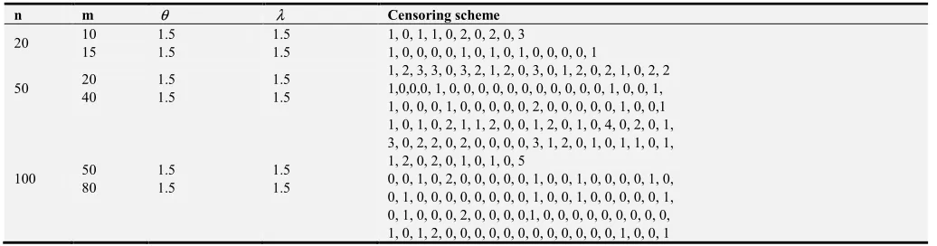
Table 1. Censoring scheme R=( , , ...., r r1 2 rm) for β θ=( =1.5, =1.5)λ .
n m θ λ Censoring scheme
20 10 15
1.5 1.5
1.5 1.5
1, 0, 1, 1, 0, 2, 0, 2, 0, 3
1, 0, 0, 0, 0, 1, 0, 1, 0, 1, 0, 0, 0, 0, 1 50 20
40
1.5 1.5
1.5 1.5
1, 2, 3, 3, 0, 3, 2, 1, 2, 0, 3, 0, 1, 2, 0, 2, 1, 0, 2, 2 1,0,0,0, 1, 0, 0, 0, 0, 0, 0, 0, 0, 0, 0, 0, 1, 0, 0, 1, 1, 0, 0, 0, 1, 0, 0, 0, 0, 0, 2, 0, 0, 0, 0, 0, 1, 0, 0,1
100 50 80
1.5 1.5
1.5 1.5
1, 0, 1, 0, 2, 1, 1, 2, 0, 0, 1, 2, 0, 1, 0, 4, 0, 2, 0, 1, 3, 0, 2, 2, 0, 2, 0, 0, 0, 0, 3, 1, 2, 0, 1, 0, 1, 1, 0, 1, 1, 2, 0, 2, 0, 1, 0, 1, 0, 5
Table 1 represents the progressive censoring scheme for different samples size and different numbers of failures for parametersβ =(θ =1.5, =1.5)λ .
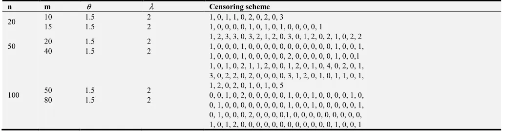
Table 2. Censoring scheme R=( , , ...., r r1 2 rm) for β θ=( =1.5, =2)λ .
n m θ λ Censoring scheme
20 10 15
1.5 1.5
2 2
1, 0, 1, 1, 0, 2, 0, 2, 0, 3
1, 0, 0, 0, 0, 1, 0, 1, 0, 1, 0, 0, 0, 0, 1 50 20
40
1.5 1.5
2 2
1, 2, 3, 3, 0, 3, 2, 1, 2, 0, 3, 0, 1, 2, 0, 2, 1, 0, 2, 2 1, 0, 0, 0, 1, 0, 0, 0, 0, 0, 0, 0, 0, 0, 0, 0, 1, 0, 0, 1, 1, 0, 0, 0, 1, 0, 0, 0, 0, 0, 2, 0, 0, 0, 0, 0, 1, 0, 0,1
100 50 80
1.5 1.5
2 2
1, 0, 1, 0, 2, 1, 1, 2, 0, 0, 1, 2, 0, 1, 0, 4, 0, 2, 0, 1, 3, 0, 2, 2, 0, 2, 0, 0, 0, 0, 3, 1, 2, 0, 1, 0, 1, 1, 0, 1, 1, 2, 0, 2, 0, 1, 0, 1, 0, 5
0, 0, 1, 0, 2, 0, 0, 0, 0, 0, 1, 0, 0, 1, 0, 0, 0, 0, 1, 0, 0, 1, 0, 0, 0, 0, 0, 0, 0, 0, 1, 0, 0, 1, 0, 0, 0, 0, 0, 1, 0, 1, 0, 0, 0, 2, 0, 0, 0, 0,1, 0, 0, 0, 0, 0, 0, 0, 0, 0, 1, 0, 1, 2, 0, 0, 0, 0, 0, 0, 0, 0, 0, 0, 0, 0, 1, 0, 0, 1
Table 2 represents the progressive censoring scheme for different samples size and different numbers of failures for parameters β =(θ=1.5, =2)λ .
Table 3. Censoring scheme R=( , , ...., r r1 2 rm) for β θ=( =2.3, =2)λ .
n m θ λ Censoring scheme
20 15 2.3 2 1, 0, 0, 1, 1, 1, 0, 0, 1, 0, 0, 0, 0, 0, 0 30 15 2.3 2 1, 0, 1, 1, 0, 1, 2, 0, 1, 2, 2, 0, 2, 0, 2 40 15 2.3 2 1, 0, 1, 1, 0, 1, 2, 5, 0, 2, 2, 3, 2, 0, 5
Table 3 represents the progressive censoring scheme for increasing samples size but fixed numbers of failures for parameters
( 2.3, =2)
β θ= λ .
No restriction has been imposed on the maximum number of iterations and convergence is assumed when the absolute differences between successive estimates are less than 10−5. All computational results were computed using R software.
Table 4. The MLEs, Variances, covariance and 95% confidence limits of the MLEs for the parameters of Poisson-exponential distribution under progressive type II censored sample whenβ θ=( =1.5, =1.5)λ
.
n m θˆ λˆ var( )θˆ var( )λˆ cov( , )λ θˆ ˆ CL(θ ) CL(λ)
LCL UCL LCL UCL
20 10 1.0349 1.4462 4.3642 0.8841 1.6737 -2.6101 5.5791 -0.3429 3.3429 15 1.6676 1.6068 2.4254 0.4323 0.8316 -1.5680 4.5370 0.2112 2.7887 50 20 1.3241 1.4792 1.6817 0.3864 0.6517 -1.0572 4.0262 0.2817 2.1783 40 1.5392 1.2672 1.1076 0.1958 0.3950 -0.5783 3.5472 0.6325 2.3675 100 50 1.8236 1.3161 0.5689 0.1184 0.1979 0.0049 2.9641 0.8257 2.1742 80 1.3900 1.5574 0.4647 0.0799 0.1572 0.1484 2.8406 0.9460 2.0540
From the above table, it is observed that irrespective of the censoring rate and at which point the censored units are removed from the sample, for increasing sample size;
a the estimated value of the parameter converge to the true value, b the variances and covariance of the MLEs decrease.
It is also observed that, for the case when n is fixed (i.e. n = 20), we note that as m increases (i.e. from 10 to 15) the variances and the covariance values decrease (also see table 5).
Table 5. The MLEs, Variances, covariance and 95% confidence limits of the MLEs for the parameters of Poisson-exponential distribution under progressive type II censored sample whenβ θ=( =1.5, =2)λ .
n m θˆ λˆ var( )θˆ var( )λˆ cov( , )λ θˆ ˆ CL(θ ) CL(λ)
LCL UCL LCL UCL
From the above table, it is observed that irrespective of the censoring rate and at which point the censored units are removed from the sample, for increasing sample size;
a the estimated value of the parameter converge to the true value.
b the variances and covariance of the MLEs decrease.
Table 6. Confidence intervals of β θ=( =1.5, =1.5)λ .
n m Width of C. I (θ ) Width of C. I (λ)
20 10 8.1891 3.6858
15 6.1049 2.5774
50 20 5.0835 2.4366
40 4.1256 1.7350
100 50 2.9591 1.3486
80 2.6722 1.1080
From the above table, it is observed that the widths of 95% confidence intervals tend to be narrower for an increasing sample size.
Table 7. Confidence intervals of β θ=( =1.5, =2)λ .
n m Width of C. I (θ ) Width of C. I(λ)
20 10 6.8227 2.4354
15 6.0596 2.3245
50 20 5.3926 1.8160
40 3.7950 1.4780
100 50 3.2693 1.1617
80 2.6512 1.0313
From the above table, it is also observed that the widths of 95% confidence intervals tend to be narrower for an increasing sample size.
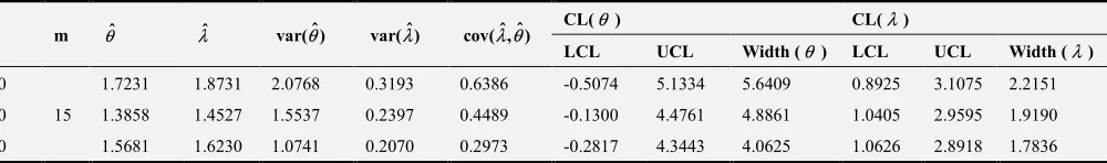
Table 8. The MLEs, Variances, covariance and 95% confidence limits of the MLEs for the parameters of Poisson-exponential distribution under progressive type II censored sample whenβ θ( =2.3, =2)λ with different sample size but fixed number of failures completely observed.
n m θˆ λˆ var( )θˆ var( )λˆ cov( , )λ θˆ ˆ CL(θ ) CL(λ)
LCL UCL Width (θ ) LCL UCL Width (λ)
20 15
1.7231 1.8731 2.0768 0.3193 0.6386 -0.5074 5.1334 5.6409 0.8925 3.1075 2.2151 30 1.3858 1.4527 1.5537 0.2397 0.4489 -0.1300 4.4761 4.8861 1.0405 2.9595 1.9190 40 1.5681 1.6230 1.0741 0.2070 0.2973 -0.2817 4.3443 4.0625 1.0626 2.8918 1.7836
From the above table, it is observed that irrespective of the censoring rate and at which point the censored units are removed from the sample with fixed number of failures completely observed for increasing sample size;
a the estimated value of the parameter converge to the true value.
b the variances and covariance of the MLEs decreases.
4. Conclusions
This study has addressed the problem of estimation of parameters of the Poisson-exponential distribution based on progressive Type-II censored data. The maximum likelihood estimators of the scale and shape parameters were obtained by using EM algorithm.
A comparison of the MLEs and their variances as well as their confidence intervals was made by simulation for different censoring schemes. It was observed that:
(i) for an increasing sample size, the estimated value of the parameter becomes closer to the true value, the variances and covariance of the MLEs decrease and the widths of the confidence intervals become narrower.
(ii) reducing the number of units to be removed in the censoring scheme, leads to better estimates for a fixed sample size.
The results provide the EM algorithm that is relatively robust against the initial values. It guarantees a single uniform non-decreasing likelihood trial from the initial value to the convergence value. Moreover, with the EM algorithm, there is no need to evaluate the first and second derivatives of the log-likelihood function, which helps save the central
processing unit (CPU) time of each iteration. The Expectation Maximization algorithm is computational stable, easy to implement and asymptotic variances and covariance of estimates are also obtained.
References
[1] Kus, C. (2007). A new lifetime distribution. Computational Statistics and Data Analysis 51, 4497-4509.
[2] Barreto, S. W. and Cribari, N. F. (2009). A generalization of Exponential-Poisson distribution. Statistics and Probability Letters 79, 2493-2500.
[3] Cancho, V. G. Louzada-Neto, F. and Barriga, G. D. C. (2011). The Poisson-Exponential lifetime distribution. Computational Statistics and Data Analysis 55, 677-686.
[4] Basu,A.,Klein, L. (1982). Some Recent Development in Competing Risks Theory. Survival Analysis,IMS, Hayward. [5] Adamidis,K.,Loukas, S. (1998). A Lifetime distribution with
decreasing failure rate. Statistics and Probability Letters 39(1), 35-42.
[6] Bain, L. T and Engelhardt, M. (1991). Statistical Analysis of Reliability and Life Testing Model, Marcel Dekker; New York. [7] Cohen. A. C. (1976). Progressively censored sampling in the three parameter lognormal distribution, Technometrics 18, 99-103.
[9] Amal, H. Samawi, H. and Mohammad, Z. R. (2013). Estimation on Lomax Progressive Censoring using E. M algorithm. The Journal of Statistical Computation and Simulation 1-18.
[10] Balakrishnan N. (2007). Progressive censoring methodology: an appraisal (with discussion). TEST;16:211–259.
[11] Louzada-Neto, F., Cancho, V. G. and Barrigac, G. D. C. (2011). The Poisson- Exponential distribution: a Bayesian approach. Journal of Applied Statistics 38, 1239-1248. [12] Singh S. K., Singh, U. and Manoj, K. M. (2014). Estimation
for the Parameter of Poisson-Exponential Distribution under Bayesian Paradigm, Journal of Data Science 12, 157-173. [13] Raqab, M. Z. and Madi, T. M. (2011). Inference for the
generalized Rayleigh distribution based on progressively censored data. Journal of Statistical Planning and Inference 141, 3313-3322.
[14] Krishna. H and Kumar (2011). Reliability estimation in Lindley distribution with progressively type II right censored sample. Mathematics and Computers in Simulation 82(2), 281-294.
[15] Kumar. K, Garg. R and Krishna, H. (2014). Estimation of parameters of Nakagami distribution with progressively censored samples. National conference on Statistical Inference, Sampling Techniques and Related Areas February, 18-19 at AMU Aligarh.
[16] Pak, A., Gholam. A. P. and Mansour. S (2014). Inference for the Rayleigh Distribution Based on Progressive Type-II Fuzzy Censored Data. Journal of Modern Applied Statistical Methods 13(1), Article 19.
[17] Rastogi, M. K. and Tripathi, Y. M. (2012). Estimating the parameters of Burr distribution under progressive type II censoring. Statistical Methodology 9,381-391.
[18] Watanable M. and Yamaguchi K. (2004). The EM algorithm and related statistical models. New York: Marcel Dekker. [19] Ng K., Chan P. S and Balakrishnan N. (2002). Estimation of
Parameters from progressively censored data using an EM algorithm. Computational Statistics and Data Analysis, 39 (4), 371-386.
[20] Rubin D. B. (1991). EM and beyond. Psychometrika 56,241– 254.
[21] Rubin D. B. (1987). The SIR algorithm. Journal of American Statistical Association 82,543–546.
[22] Tanner M. A and Wange W. H. (1987). The calculation of posterior distributions by data augmentation. Journal of American Statistical Association 82,528–550.
[23] Balakrishnan, N. and Aggarwala, R. (2000). Progressive censoring: theory, methods, and applications. Birkhäuser, Boston.
[24] Dempster, A. P, Laird, N. M and Rubin, D. B. (1977). Maximum likelihood from incomplete data via the EM algorithm. Journal of the Royal Statistical Society, 39(1), 1– 38.
[25] McLachlan, G. J. and Krishnan, T. (1997). The EM Algorithm and Extension. Wiley, New York.
[26] Sadegh, R. and Rasool, T. (2012). A New Lifetime Distribution with Increasing Failure Rate: Exponential Truncated Poisson. Journal of Basic and Applied Scientific Research 2(2), 1749-1762.
[27] Cox, D. and Hinkley, D. (1979). Theoretical statistics, Chapman & Hall, London.