www.ann-geophys.net/32/581/2014/ doi:10.5194/angeo-32-581-2014
© Author(s) 2014. CC Attribution 3.0 License.
Criterion for analyzing experimental data on eddy diffusion
coefficients
M. N. Vlasov and M. C. Kelley
School of Electrical and Computer Engineering, Cornell University, Ithaca, NY, USA Correspondence to: M. N. Vlasov ([email protected])
Received: 31 May 2013 – Revised: 12 April 2014 – Accepted: 15 April 2014 – Published: 2 June 2014
Abstract. Problems exist in estimating the eddy heat trans-port coefficient, Keh, from experimental data. These
prob-lems are due to uncertainty in determining the turbulent en-ergy dissipation rate and to the uncertainty of Keh
depen-dence on the energy dissipation rate. In this paper, a new criterion for estimating the eddy heat transport coefficient is suggested. This criterion is based on the effect of eddy turbulence on the energy budget of the upper mesosphere and lower thermosphere. The calculations show high cool-ing around and above theKeh peak forKehvalues inferred
from experimental data. The cooling rates are much higher than cooling rates corresponding to the temperature given by the MSIS-E-90 model or to temperatures measured during the experiments. The main contribution to high cooling rates is due to the term with eddy heat conduction, which strongly depends on the Keh gradient. According to our results, the
heating/cooling values below the Keh peak altitude
corre-spond to the temperature given by the MSIS-E-90 model, but at the peak and above, the cooling rates are larger by a fac-tor of 2–3 than the rates corresponding to the temperatures. This means that the Keh values in the peak and above may
be overestimated. Application of this criterion to the Turbu-lent Oxygen Mixing Experiment (TOMEX) data shows that eddy diffusions inferred from observing chemical tracers in TOMEX are strongly overestimated.
Keywords. Atmospheric composition and structure (middle atmosphere – composition and chemistry) – meteorology and atmospheric dynamics (middle atmosphere dynamics; turbu-lence)
1 Introduction
A number of ground-based and in situ measurement tech-niques for estimating the eddy diffusion coefficient Ked
or eddy heat transport coefficient Keh exist. Note that the
term “eddy diffusion coefficient” is frequently used instead of “eddy heat transport coefficient” in the literature. Radar measurements of the Doppler spectra width or the absolute strength of backscattered power are used to derive the eddy diffusion coefficients (Hocking, 1987). Using ground-based measurements of the green line emission, the eddy diffusion coefficient has been derived. This method is based on the ef-fect of turbulence on the atomic oxygen responsible for the green line emission. Meteor trail observations are used to es-timate the eddy diffusion coefficient (Kelley et al., 2003).
Rocket measurements of neutral and electron density fluc-tuations are used to infer the eddy diffusion coefficient (Lübken, 1997). The density fluctuation is similar to a pas-sive natural tracer variation induced by turbulence. An-other rocket-borne technique uses chemiluminescent clouds as tracers released from rockets (Rees et al., 1972; Roper, 1996). All of these methods have limitations and require some theoretical assumptions. The main assumption is lin-ear dependence of the energy dissipation rate on the product of the eddy diffusion coefficient and the square of the buoy-ancy frequency. Problems with applying this fairly restrictive assumption were noted many times (for example, Fritts and Luo, 1995; Lübken, 1997; Hocking, 1999). We return to this problem later.
582 M. N. Vlasov and M. C. Kelley: Criterion for analyzing experimental data on eddy diffusion coefficients
Our paper is organized as follows. The main uncertain-ties in determining the eddy diffusion coefficient from exper-imental data are discussed in Sect. 2. Analysis of eddy dif-fusion coefficients Keh inferred from rocket measurements
of density fluctuations and rocket-borne chemical tracer re-leases is presented in Sects. 3 and 4. This analysis is based on estimating the effect of eddy heat transport (eddy diffusion) on the thermal balance in the mesosphere and lower thermo-sphere (MLT) using the equation for heating/cooling rates by eddy turbulence. The suggested criterion requires agreement between the cooling rate induced by eddy turbulence and the cooling rate corresponding to the temperature given by the MSIS-E-90 model.
2 Uncertainty of an eddy diffusion coefficient inferred from experimental data
The energy dissipation rate, ε, is a key parameter in deter-mining the eddy diffusion coefficient,Ked, from
experimen-tal data. Usually, the spectrum of density fluctuations calcu-lated from experimental data is approximated using the the-oretical model of Heisenberg (1948) and the inner scale,l0,
is determined. This parameter is related to the Kolmogorov microscale,η, through the relationl0=9.9η(Lübken et al.,
1993). The Kolmogorov microscale is a rough estimate of the size of the smallest eddies, which can provide the turbu-lent energy dissipation by viscosityν. Then theεvalue can be calculated using the formulaε=ν3η−4. According to this formula, theεvalue strongly depends on theηvalue, which is estimated by a rough approximation. For example, let us estimate the impact ofηvalues on the energy dissipation rate using the l0 values inferred from the experimental data by
Kelley et al. (2003). These values vary from 156 to 222 m, and the εvalue can change from 0.14 to 0.58 W kg−1. Us-ing the formulaKed=bε/ω2Bwithb=0.8 derived by
Wein-stock (1978) whereωBis the buoyancy frequency, Kelley et
al. (2003) estimated theKedaveraged value to be 500 m2s−1.
Taking into account theεvariation estimated above, theKed
maximum values can vary from 250 to 1000 m2s−1, cover-ing allKedmaximum values measured in the mesosphere and
lower thermosphere (Fukao et al., 1994). However, it is dif-ficult to imagine that limited experimental data from observ-ing a few meteor trails (Kelley et al., 2003) could present the whole range of Kednatural variations. In this case, the
accuracy of the microscale estimate can play an important role. Note that theηchange by 20 % corresponds to theKed
change by a factor of 2.
The other uncertainty results from the application of for-mula Ked=0.8ε/ωB2 (∗) (Weinstock, 1978) and the
for-mula Kedω2B(P−Ri) /Ri=ε(∗∗) whereP and Ri are the
Prandtl and Richardson numbers, respectively. Equation (∗∗) is derived assuming a balance between the rate of energy transferred from the mean motion to the fluctuations on one side and the rates of turbulent energy dissipation due
to viscosity and buoyancy force on the other side in a steady state (Chandra, 1980; Gordiets et al., 1982). This bal-ance assumes that the fluctuations are stationary, homoge-neous, and isotropic. However, these conditions are scarcely probable in the real atmosphere. The Eq. (∗) derived by Weinstock (1978) is also for stratified homogeneous turbu-lence. However, this relation is commonly used to estimate Kehfromε. There is no evidence of any advantage in using
Eqs. (∗) or (∗∗), but the latter has an additional problem with Ri determination.
The Prandtl number is equal to 1 for uniform turbulence and Ri=0.44 for b=0.81. The Kelvin–Helmholtz insta-bility requires Ri≤0.25, corresponding to b≤0.3. Equa-tion (∗) with b=0.3 was obtained by Lilly et al. (1974). However, Weinstock (1978) assumed that the turbulence pro-duced in regions of dynamic instability (Ri≤0.25) will be transported by turbulent flux into the regions of larger Ri, and the Ri mean value may be 0.44. Lübken (1997), using Eq. (∗), notes that the derivation of this formula relies on fairly restrictive assumptions concerning the turbulent field. Note that abvalue equal to 0.8 is used to estimate theKed
value in all experimental data. The problem when applying Eqs. (∗) and (∗∗) is considered in detail by Hocking (1999).
The same problem exists in estimating the energy dissipa-tion rate inferred from chemical tracer observadissipa-tions. In this case, formulaε=rt2t−3/(2.4α)1.5(Rees et al., 1972, and ref-erences therein) is usually used. Here,rt is the trail radius
as a function of time,t, and α is a Kolmogorov constant. The values of this constant vary between 0.5 and 1.5 because the absolute value is unknown (Rees et al., 1972; Weinstock, 1978). In this case, theεvalue can change by a factor of 5 due to the uncertainty of a Kolmogorov constant. Note that Bishop et al. (2004) had to use theαmaximum value because the energy dissipation rates inferred from the chemical tracer dynamics were unusually high. We will discuss the results of this experiment in Sect. 4. Thus, the uncertainty of the eddy diffusion coefficient inferred from experimental data is a fac-tor of 3.
3 Analysis of eddy diffusion coefficients inferred from rocket measurements of density fluctuations
Using the equation for the heating/cooling rates ofQed
in-duced by eddy turbulence, it is possible to estimate these rates for different eddy heat transport coefficients of Keh.
Note that the term “eddy diffusion coefficient” is frequently used instead of Keh. TheQed estimates show that cooling
takes place around and above theKeh peak. The suggested
criterion is based on comparing the calculated cooling rates with normal cooling rates corresponding to the measured temperatures generalized by the MSIS-E-90 model. The en-hancement of the cooling induced by eddy turbulence means that theKehvalues inferred from experimental data are too
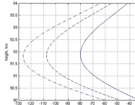
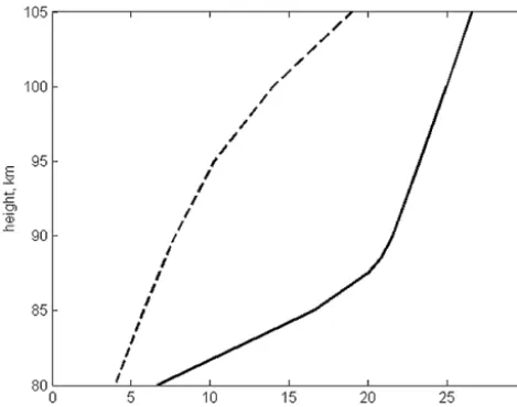
Figure 1. The eddy diffusion coefficient inferred by L97 in polar summer (solid curve) and approximated by Eqs. (2) and (3) (dashed curve). The horizontal dashed line shows theKedpeak altitude.
of theKehvalues for theKehheight profile inferred from
ex-perimental data. It must be emphasized that the Qed value
depends on both theKehvalues and the gradientKehvalues.
Therefore, both parameters must meet the criterion.
The cooling/heating volume rate corresponding to the eddy diffusion coefficient can be estimated using the equa-tion (Vlasov and Kelley, 2010)
Qed=
∂ ∂z
KehCpρ
∂T
∂z + g Cp
+Kehρ
g T b
∂T
∂z + g Cp
, (1)
whereQed is given in erg cm−3s−1,ρ is the density,Cp is the heat capacity at constant pressure,T is the temperature, andgis the gravitational acceleration.
Note that it is usually assumed that the eddy diffusion coefficient, Ked, is equal to the eddy heat transport
co-efficient, Keh. The eddy diffusion coefficient inferred by
Lübken (1997, hereafter referred to as L97) from measure-ments of the turbulent energy dissipation rate in the sum-mer polar mesosphere can be approximated by formulas sug-gested by Shimazaki (1971):
Keh=Keh0 exp [S1(z−zm)]+
Kehm−Keh0
exph−S2(z−zm)2 i
z < zm, (2)
Keh=Kehmexp h
−S3(z−zm)2 i
[image:3.612.50.287.66.252.2]z > zm, (3) where Kehm=1.83×106cm2s−1 is the maximum of these coefficients, Keh0 =7×105cm2s−1 is the value at 83 km
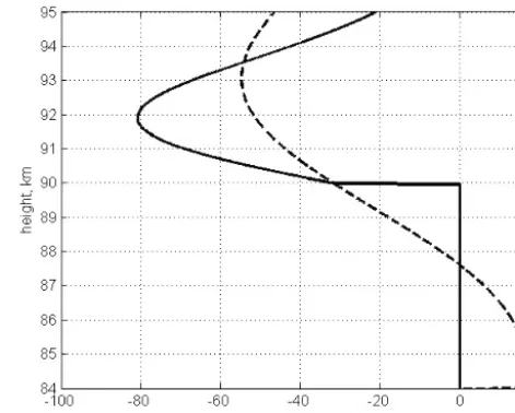
Figure 2. Cooling rates calculated with the eddy heat transport co-efficient shown in Fig. 1 with temperature gradientG=5 K km−1 (dotted-dashed curve) corresponding to the temperature height pro-file shown in Fig. 3, G=3 K km−1 (dashed curve), and G=0 (solid curve).
according to L97, andzm=90 km, S1=0.05 km−1, S2=
0.03 km−2, andS
3=0.1 km−2are free parameters. As seen
in Fig. 1, these formulas provide an excellent approximation of the eddy diffusion coefficient presented in Table 3 in L97. Using Eq. (1) with this approximation, it is possible to cal-culate the cooling/heating rates induced by eddy turbulence. The height profiles of these rates are shown in Fig. 2. Strong cooling takes place above the eddy diffusion coefficient peak and depends on the temperature gradient. The temperature height profile given by the MSIS-E-90 model for conditions corresponding to measurements of L97 is shown in Fig. 3. According to L97, the eddy diffusion coefficient peak is in the mesopause at 90 km. The value of this coefficient is de-termined using the formula
Ked=0.8ε/ωB2, (4)
whereωBis the buoyancy frequency given by the formula
ωB2= g T
∂T
∂z + g Cp
. (5)
Using Eqs. (4) and (5), the ε andKed values given in
584 M. N. Vlasov and M. C. Kelley: Criterion for analyzing experimental data on eddy diffusion coefficients
Figure 3. Temperature height profile given by the MSIS-E-90 model under conditions corresponding to the eddy diffusion coef-ficient inferred by L97 in polar summer and shown in Fig. 1.
Fig. 2. By comparing these cooling rates with the cooling rates shown in Fig. 10 corresponding to measured tures generalized by the MSIS-E-90 model and the tempera-ture used by L97, we see that theKehvalue does not
corre-spond to the atmospheric conditions. Other heating processes occurring in the MLT cannot compensate for these very high cooling rates. Note that this cooling strongly depends on the Kedgradient above theKedpeak, as seen in Fig. 4. The
cool-ing decreases with decreases in theKedgradient. However, in
this case, the turbopause altitude significantly increases (see Fig. 5).
In any case, strong cooling occurs above and below the Ked peak (see Fig. 4). This result contradicts one of the
main results of L97 concerning strong heating by eddy turbu-lence in the summer polar mesopause, meaning that a serious problem exists with the eddy diffusion coefficient estimation method used by L97.
As seen in Fig. 4, the altitude of the maximum heating corresponding to this coefficient is 5 km lower than theKed
peak altitude. Note that the maximum heating rate measured by L97 is 13.5 K day−1, very close to the maximum heating rate of 17 K day−1shown in Fig. 4. This means that theKed
maximum value estimated by L97 corresponds not to the al-titude of the peak eddy diffusion coefficient in L97, but to the Kedvalue at altitudes below 5 km, theKedpeak.
Considering Eq. (1) in detail, it is possible to show that cooling is in theKehpeak. Equation (1) forQed in units of
K day−1for dT /dz=0 andz≤zmcan be written as
QKed=p
S1−
1 H +
g T cCp
Keh0 exp [S1(z−zm)]
−p
2S2(z−zm)+ 1 H−
g T cCp
Kehm−Keh0
Figure 4. Height profiles of the cooling rates calculated by Eq. (1) with the eddy heat transport coefficient inferred by L97 in summer (solid curve) andS3=S2=0.03 km−2(dashed curve), dT /dz=0, Keh0 =0, andS1=0. The horizontal solid line shows the altitude of theKehm peak, and the vertical solid line shows the boundary be-tween cooling and heating.
exph−S2(z−zm)2 i
, (6)
wherep=gτd/Cv. The Qed value is negative at the Keh
peak altitude because the scale heightH< 8 km in the MLT and 1/H> (S1+g/T cCp). Cooling above theKehpeak
alti-tude is due to theKehnegative gradient.
We suggest that theKehm value can be estimated using the thermal balance equation
KehCp
∂2T ∂z2 +Cp
∂K eh
∂z + Ke
ρ ∂ρ ∂z
∂T
∂z
+g ∂K
eh
∂z + Keh
ρ ∂ρ ∂z
+ε+q−L=0, (7) which includes the first term of Eq. (1) divided by mass den-sityρ, heating due to the energy dissipation of gravity waves, ε, chemical heating and heating by ultraviolet solar radiation, q, and cooling by CO2and O infrared radiation,L.
Note that (1/ρ)∂ρ/∂/z= −1/H for ∂T /∂z=0 and (1/ρ)∂ρ/∂/z= −(α+mg/κ)/(T0+αz), where m is the
mass, for∂T /∂z=α. According to the conditions in L97, theKedpeak is in the mesopause (∂T /∂z=0) and Eq. (7)
can be simplified to the relation
Kehmg/H=q+ε−L. (8)
Using this relation with theεvalue given in Table 3 in L97 at theKed peak altitude and (q−L) ≤10 K day−1,Kehm is
[image:4.612.310.546.66.255.2]Figure 5. The eddy diffusion coefficient (L97) (solid curve) with S3=0.03 km−1(dashed curve) and the molecular diffusion coeffi-cient (dotted-dashed line). The horizontal line shows the altitude of theKehpeak.
due to the largeS3value corresponding to theKedheight
pro-file given by L97. TheS3value should decrease by a factor
of 10 to maintain thermal balance at altitudes above theKed
peak. However, in this case, the turbopause altitude can be too high.
Thus, in this case, the cooling induced by the eddy diffu-sion measured by Lübken is very large, resulting in aP value larger than 2 and localized turbulence.
4 Analysis of eddy diffusion coefficients inferred from a rocket-borne chemical tracer experiment
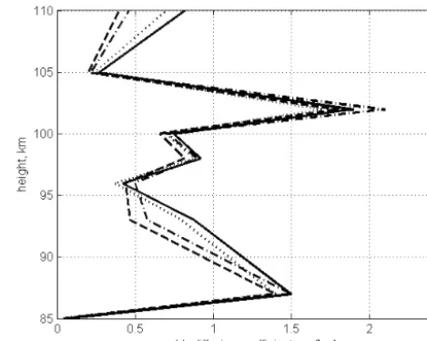
We now consider estimates of the eddy diffusion coefficient inferred from observing chemical tracers during a rocket-borne experiment (Bishop et al., 2004, hereafter referred to as B04). The energy dissipation rate and the eddy diffu-sion coefficients calculated by Eq. (4) are given in Tables 1 and 2 in B04. Height profiles of the eddy diffusion coeffi-cients given in Table 2 are shown in Fig. 6. These profiles have two peaks at 87 and 102 km altitude. The steep, neg-ative temperature gradients were observed in these peaks, and the temperatures can be described by the linear func-tionT (z)=T0−αz, as seen in Fig. 2 in Hecht et al. (2004).
Using Eq. (7) and (1/ρ)∂ρ/∂/z= −(α+mg/κ)/(T0+αz)
for∂T /∂z= −α,∂2T /∂z2=0 and∂Keh/∂z=0 in theKeh
peak, it is possible to obtain the formula
Kehm= (ε+q−L)T
Cp(P−α)(g/Cp−α), (9)
whereP =T /H. Equation (4) is used by B04 to estimate the Kehm value. Using Eq. (9) and theεandKehmvalues at 87 km,
Figure 6. Height profiles of eddy diffusion coefficients inferred from the rocket-borne chemical tracer experiment given in Table 2 for methods 1–4 (Bishop et al., 2004) are shown by solid, dashed-dotted, dashed-dotted, and dashed lines, respectively.
as given in Tables 1 and 2 in B04,ω2Bcan be found. Then the temperature gradient can be estimated to be−8 K km−1 within the height range of 86 to 95 km by using the temper-ature height profile shown in Fig. 2 in Hecht et al. (2004), and Kehm=7.7×106cm2s−1 can be found. This value is less by a factor of about 2 than theKehm=1.5×107cm2s−1 value estimated by Bishop et al. (2004). This difference shows that a problem exists with the application of Eq. (4). We discuss this problem later. The cooling rates calculated withKehm=1.5×107cm2s−1and theK
ehapproximation by
Eq. (3) within the altitude range of 87–96 km are shown in Fig. 7. This cooling would be in agreement with the strong negative temperature gradient estimated above if it did not contradict the very high temperature measured just below theKehpeak (see Hecht et al., 2004). A very strong source
of heating is necessary to increase the temperature by 35 K, higher than normal temperatures at 85 km altitude. Note that the eddy turbulence can heat the atmosphere above theKeh
peak if convective instability (−∂T /∂z>g/Cp) occurs. It is possible to assume that this instability took place before the observations.
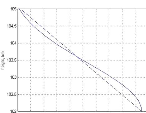
We now consider the eddy diffusion coefficients inferred by Bishop et al. (2004) at 102–105 km altitude and shown in Fig. 6 withKehm=2.1×107cm2s−1. The height
distribu-tion approximadistribu-tion of thisKehby Eq. (3) and the linear
de-pendence are shown in Fig. 8. Using the approach described above, it is possible to estimate the temperature gradient used in Eq. (4) by Bishop et al. (2004) for their estimates of the Keh values. The cooling rate height profile calculated with
theKehapproximation by Eq. (3) is shown in Fig. 9. These
[image:5.612.50.286.66.253.2]586 M. N. Vlasov and M. C. Kelley: Criterion for analyzing experimental data on eddy diffusion coefficients
Figure 7. Height profiles of cooling rates corresponding to theKehm value estimated by Bishop et al. (2004) at 87 km and the exponential approximation of theKehheight profile above the peak with theKeh gradient, S3, equal to 0.015 km−2 (solid curve) and 0.016 km−2 (dashed-dotted curve).
Figure 8. The approximation by Eq. (3) (solid curve) and the linear approximation (dashed line) of the eddy diffusion coefficients given in Table 2 in Bishop et al. (2004) within the altitude range of 102– 105 km.
realistic. The cooling calculated with the linear approxima-tion is a little smaller but is also too high.
Finally, our analysis shows that the eddy diffusion coeffi-cients inferred from observing chemical tracers are overesti-mated. Note that the coefficients used by TIME-GCM to pro-vide a better fit to the Turbulent Oxygen Mixing Experiment (TOMEX) photometer data do not exceed 3×106cm2s−1.
[image:6.612.52.285.66.253.2]The results presented above mean that a contradiction ex-ists between Eq. (4), commonly used to estimate the eddy dif-fusion coefficient from experimental data, and the real eddy
Figure 9. Cooling rates calculated with theKeh approximation shown in Fig. 8 (solid curve).
turbulence. Hocking (1999) discussed this problem in detail and concluded that the application of this formula depends on the eddy scales. However, it seems to us that Hocking and the other authors use the term “eddy diffusion” in ex-tended interpretations, including diffusion with scales com-pared to atmospheric scales. We believe that eddy diffusion is the process that meets the main diffusion criterion: eddy scales are much less than the density gradient scale. This dif-fusion can only be used in difdif-fusion equations and can induce small fluctuations of mass density but cannot induce mass density transport. Large-scale diffusion can be considered as the mass transport (advection), which can induce a change of total density and can be described by the momentum equa-tion.
5 Conclusions
Deriving the eddy heat transport (eddy diffusion) coefficient from experimental data is a very complicated problem. There are two main uncertainties: (i) estimating the turbulent en-ergy dissipation rate and (ii) determining the dependence of the heat transport coefficient on the energy dissipation rate. TheKehvalue can be underestimated or overestimated by a
factor of 2–4 due to these uncertainties. Thus, an independent criterion for theKehvalue estimate can be useful.
[image:6.612.50.285.339.521.2]Figure 10. Normal cooling rates corresponding to MSIS-E-90 data for the conditions in B04 (dashed curve) and L97 (solid curve).
or contradiction to the atmospheric temperatures can be ob-tained.
The simplified formulas based on the energy rate equation can be used to estimate the eddy diffusion coefficient from the energy dissipation rate given by the experimental data. These formulas give the eddy diffusion coefficients, which are significantly less than the coefficients estimated by the commonly used Eq. (4).
Applying this criterion to the eddy diffusion coefficient in-ferred from the rocket experimental data on density fluctua-tions, L97 shows that the eddy diffusion coefficients inferred from density fluctuations (L97) at theKedpeak altitude and
below meet our criterion. However, the cooling rate above the peak is too large due to the very steep gradient of this co-efficient. The cooling rates calculated with the coefficients, estimated using chemical tracers in TOMEX (Bishop et al., 2004), are very high due to the large Kehvalue in the peak
and the very steep gradient above the peak. These coefficients are significantly overestimated. The main problem with this technique is that the non-turbulent effects can influence the tracer dynamic. For example, the molecular diffusion coef-ficientDmestimated by B04 is 1.6×107cm2s−1at 116 km
and 2.1×107cm2s−1and 2.6×107cm2s−1at 128 km. As is well known, the molecular diffusion coefficient is propor-tional to the reciprocal of the total density. In this case, the Dmvalue should increase by a factor of 3 within the altitude
range of 116–128 km. Also, theDmvalue increases with
in-creasing temperature. The estimated totalDmincreases by a
factor of 3.5, a factor of 2 larger than the Dm increase
es-timated in B04. We believe that the suggested criterion can encourage the B04 authors to reconsider their results.
Acknowledgements. Work at Cornell was supported by the National
Science Foundation under grant ATM-0551107.
Topical Editor R. Neale thanks two anonymous referees for their help in evaluating this paper.
References
Bishop, R. L., Larsen, M. F., Hecht, J. H., Liu, A. Z., and Gard-ner, C. S.: TOMEX: Mesospheric and lower thermospheric dif-fusivity and instability layers, J. Geophys. Res., 109, D02S03, doi:10.1029/2002JD003079, 2004.
Chandra, S.: Energetics and thermal structure of the middle atmo-sphere, Planet. Space Sci., 28, 585–593, 1980.
Fritts, D. C. and Luo, Z.: Dynamical and radiative forcing of the summer mesopause circulation and thermal structure, J. Geo-phys. Res., 100, 3119–3128, 1995.
Fukao, S., Yamanaka, M. D., Ao, N., Hocking, W. K., Sato, T., Ya-mamoto, M., Nakamura, T., Tsuda, T., and Kato, S.: Seasonal variability of vertical eddy diffusivity in the middle atmosphere, J. Geophys. Res., 99, 18973–18987, 1994.
Gordiets, B. F., Kulikov, Yu. N., Markov, M. N., and Marov, M. Ya.: Numerical modeling of the thermospheric heat budget, J. Geophys. Res., 87, 4504–4514, 1982.
Hecht, J. H., Liu, A. Z., Walterscheid, R. L., Roble, R. G., Larsen, M. F., and Clemmons, J. H.: Airglow emissions and oxygen mixing ratios from the photometer experiment on the Turbulent Oxygen Mixing Experiment (TOMEX), J. Geophys. Res., 109, D02S05, doi:10.1029/2002JD003035, 2004.
Hedin, A. E.: Extension of the MSIS thermosphere model into the middle and lower atmosphere, J. Geophys. Res., 96, 1159–1172, 1991.
Heisenberg, W.: Zur statistischen Theorie der Turbulenz, Z. Phys., 124, 628–657, 1948.
Hocking, W. K.: Turbulence in the region 80–120 km, Adv. Space Res., 7, 171–181, 1987.
Hocking, W. K.: The dynamical parameters of turbulence theory as apply to middle atmosphere studies, Earth Planets Space, 51, 525–541, 1999.
Kelley, M. C., Kruschwitz, C. A., Gardner, C. S., Drummond, J. D., and Kane, T. J.: Mesospheric turbulence measurements from persistent Leonid meteor train observations, J. Geophys. Res., 108, 8454, doi:10.1029/2002JD002392, 2003.
Lilly, D. K., Wasco, D. E., and Adelfang, S. I.: Stratospheric mixing estimated from high-altitude turbulence measurements, J. Appl. Meteorol., 13, 488–493, 1974.
Lübken, F. J.: Seasonal variation of turbulent energy dissipation rates at high latitudes as determined by in situ measurements of neutral density fluctuations, J. Geophys. Res., 102, 13441– 13456, 1997.
Lübken, F. J., Hillert, W., Lehmacher, G., and von Zahn, U.: Experi-ments revealing small impact of turbulence on the energy budget of the mesosphere and lower thermosphere, J. Geophys. Res., 98, 20369–20384, 1993.
588 M. N. Vlasov and M. C. Kelley: Criterion for analyzing experimental data on eddy diffusion coefficients
Roper, R. G.: Rocket vapor trail releases revisited: Turbulence and the scale of gravity waves: Implications for the imaging Doppler interferometry/incoherent scatter radar controversy, J. Geophys. Res., 101, 7013–7017, 1996.
Shimazaki, T.: Effective eddy diffusion coefficient and atmospheric composition in the lower thermosphere, J. Atmos. Terr. Phys., 33, 1383–1401, 1971.
Vlasov, M. N. and Kelley, M. C.: Estimates of eddy turbulence con-sistent with seasonal variations of atomic oxygen and its possible role in the seasonal cycle of mesopause temperature, Ann. Geo-phys., 28, 2103–2110, doi:10.5194/angeo-28-2103-2010, 2010. Weinstock, J.: Vertical turbulent diffusion in a stably stratified fluid,