www.ann-geophys.net/34/1175/2016/ doi:10.5194/angeo-34-1175-2016
© Author(s) 2016. CC Attribution 3.0 License.
Observations of diffusion in the electron halo and strahl
Chris Gurgiolo1and Melvyn L. Goldstein2
1Bitterroot Basic Research, Hamilton, Montana, USA
2Heliospheric Physics Laboratory, Code 672, NASA Goddard Space Flight Center, Greenbelt, MD, USA Correspondence to:Chris Gurgiolo ([email protected])
Received: 16 June 2016 – Revised: 24 October 2016 – Accepted: 9 November 2016 – Published: 15 December 2016
Abstract.Observations of the three-dimensional solar wind
electron velocity distribution functions (VDF) using φ–θ plots often show a tongue of electrons that begins at the strahl and stretches toward a new population of electrons, termed the proto-halo, that exists near the projection of the mag-netic field opposite that associated with the strahl. The en-ergy range in which the tongue and proto-halo are observed forms a “diffusion zone”. The tongue first appears in energy generally near the lower-energy range of the strahl and in the absence of any clear core/halo signature. While the φ– θ plots give the appearance that the tongue and proto-halo are derived from the strahl, a close examination of their den-sity suggests that their source is probably the upper-energy core/halo electrons which have been scattered by one or more processes into these populations.
Keywords. Interplanetary physics (solar wind plasma)
1 Introduction
The electron portion of the solar wind consists of four distinct populations: a thermal isotropic core (Feldman et al., 1975), a suprathermal halo (Feldman et al., 1975), a high-energy super-halo (Lin, 1998; Wang et al., 2012), and a field-aligned strahl (Rosenbauer et al., 1976, 1977). The general consen-sus is that the initial formation of the electron solar wind oc-curs in the corona through a combination of Coulomb colli-sions and wave–particle interactions (e.g., see Vocks et al., 2008; Vocks, 2012; Pavan et al., 2013; Che and Goldstein, 2014; Che et al., 2014) resulting in a core population and a beam-like suprathermal tail. The formation of the observed halo comes through a combination of Coulomb interactions of the beam-like suprathermal tail and either local whistler and/or kinetic Alfvén wave turbulence (Vocks et al., 2005). Che and Goldstein (2014) have suggested that the required
turbulence is generated from counterstreaming electrons pro-duced in nanoflares. The strahl arises from the fraction of the beam-like suprathermal tail that is collisionless – those par-ticles are strongly focused by the magnetic field into a beam propagating along the local field while the lower-energy core and halo move with the protons radially outward. Recently, Seough et al. (2015) have proposed that the strahl is formed directly from the halo via pitch-angle scattering. Simulations that do not include wave–particle interactions or turbulence have been run by Landi et al. (2012) with results closely matching observations. The simulations are run between 0.3 to 6.0 AU, well above the exosphere, and show the impor-tance of Coulomb collisions. This does not, however, imply that wave–particle interactions and turbulence are unimpor-tant as the simulations begin outside the corona, where it has been suggested that these processes will play a major role in determining the properties of the solar wind.
charac-teristics are required during these times, then numerical fit-ting is necessary.
Interactions between interplanetary medium and the so-lar wind (especially the strahl) as it expands and propagates away from the sun are thought to be responsible for a number of observed effects. In the absence of collisions, focusing by the mirror force should narrow the strahl; however, in actual-ity the strahl is observed to broaden with radial distance from the sun (Pilipp et al., 1987a, b; Hammond et al., 1996). The broadening begins where pitch-angle scattering would be ex-pected to dominate over focusing (∼0.5 AU) (Owens et al., 2008). There are a number of sources of free energy in the so-lar wind (e.g., see Dum et al., 1980; Saito and Gary, 2007b, a; Gary and Saito, 2007; Gary et al., 2008; Viñas et al., 2010) available to drive the pitch-angle scattering. These include interactions of the strahl with sunward-propagating whistler waves (e.g., Vocks et al., 2008), scattering off of broadband whistler turbulence (Pierrard et al., 2011), and scattering by Langmuir waves (Pavan et al., 2013).
In addition to pitch-angle broadening of the strahl, Mak-simovic et al. (2005) and Stverák et al. (2009) have shown that the strahl and halo densities vary in opposite directions with radial distances from the sun (the density of the strahl decreases in conjunction with an increase in the halo). This suggests that at least a portion of the strahl may be being degraded in energy and merged into the halo. The processes active in driving this are unknown, but it has been suggested that they include at least some of the same processes respon-sible for the broadening of the strahl. This is seen as a slow and continual erosion of the strahl and buildup of the halo through inelastic scattering.
Gurgiolo et al. (2012) have shown observations of what appears to be a strong local diffusion of the strahl in a re-stricted energy band where the strahl and halo overlap. This is an overlap in energy but not necessarily in the angular di-mensions (of velocity space) and suggests that the buildup of the halo may not be a slow and steady process but may occur in “quantum” jumps within regions where the intense disruption of the lower edge of the strahl occurs. Any pro-cesses that may be involved in setting up the diffusion over and above those associated with pitch-angle broadening have yet to be identified.
In this paper we take a closer look at the diffusion signa-tures reported by Gurgiolo et al. (2012). Data from a number of different time intervals are looked at specifically in regard to how the diffusion signature varies with energy and the for-mation and characteristics of the proto-halo (a population of electrons that is formed in the diffusion zone) and the waves present within the regions where the diffusion is observed. Surprisingly, looking at the densities of the individual elec-tron populations within the diffusion zone suggests that is not the strahl being disrupted as originally postulated by Gurgi-olo et al. (2012) but the upper-energy halo electrons. It is the disruption of this population that apparently is the source of the electrons observed in the diffusion zone.
Z11 Z10
Z9 Z8
Z7 Z6
Z5
Z4
Z3
Z2
Z1 Z0
-Z GSE
Spin Axis
GSE X
Sun
• 0 deg phase angle
[image:2.612.312.540.67.241.2]Sun in XZ plane
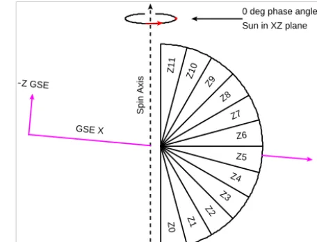
Figure 1.Schematic applicable to either of the two PEACE instru-ment heads showing the 12 elevation zones and their aligninstru-ment in the PEACE frame of reference. The PEACE frame of reference is within 5◦of GSE.
2 Data
This study uses data from multiple Cluster experiments, gen-erally taken from the spacecraft with the cleanest data sets during the time being studied. The cleanest data are generally from either C1, which has the best proton data, or C2, which usually has the best electron data up to late May 2011 when there was a failure in the one of elevation zone sensors. We have restricted ourselves in this paper to time periods when the spacecraft were returning data using burst-mode teleme-try. During those times the returned data are generally at or close to their highest resolution.
The electron data come from the Plasma Electron And Current Experiment (PEACE) (Johnstone et al., 1997; Faza-kerley et al., 2010). Figure 1 shows a schematic applicable to either of the two PEACE heads, which are mounted 180◦ apart on the spacecraft body. The figure is drawn in the in-strument frame of reference and for comparison includes the GSEZandXaxes. Each head consists of a fan of 12 eleva-tion zones mounted parallel to the spacecraft spin axis. The spin axis is aligned to within 5◦of−ZGSE, which tilts the GSE ecliptic plane by−5◦in the figure. The instrument uses the spacecraft spin to scan velocity space in azimuth. In the instrument frame of reference the 0◦azimuth angle defines the location at which the fan of sensors is in the plane de-fined by the GSEXZ axes (the plane containing the sun). Most of the data in this study come from the low-energy electrostatic analyzer (LEEA) head, but there are some data intervals when the data come from the high-energy electro-static analyzer (HEEA). The major difference between the two heads is that HEEA has a larger geometric factor.
Spatio-Temporal Analysis of Field Fluctuations (STAFF) (Cornilleau-Wehrlin et al., 1997, 2010) to produce magnetic field power spectra. Five vector per second FGM data are used to indicate the location of the projections of the mag-netic field head and tail locations in all the phi-theta (φ–θ) plots used in the paper.
The spacecraft potential data are used to correct the mea-sured energy in moment estimates and were provided by the Electric Field and Waves (EFW) experiment (Gustafsson et al., 1997; Khotyaintsev et al., 2010).
In burst-mode telemetry PEACE returns a continuous set of full 3-D eVDFs with a time resolution of the spacecraft spin rate (∼4 s). The energy and angular resolutions, how-ever, are variable and depend on the instrument mode, but in general the data come from 32 azimuth sectors, 6 or 12 elevation sectors, and 30 or 60 energy steps. To obtain the highest resolution (time, energy, and angular) within the dif-fusion energy range, we used burst-mode data of all the anal-yses within this paper. In burst-mode telemetry the FGM full-resolution magnetic field data are generally sampled at 67 vectors per second and the STAFF waveform data at 450 vectors per second. This allows spectra to be computed through the ion scale length and down toward electron scales. With the exception of PEACE data, which was obtained from the Mullard Space Science Laboratory (MSSL) science data archive, all data were obtained from the Cluster Science Archive (CSA, http://www.cosmos.esa.int/web/csa).
3 φ–θplots
φ–θ plots are used throughout to illustrate features in the electron eVDFs. This mode of presentation allows one to show the entire three-dimensional distribution function at a given energy as a two-dimensional projection. We discuss its primary features and some caveats of which the general user should be aware.
A φ–θ plot shows data within a spherical shell in phase space associated with a single returned energy step. The data are plotted in the instrument frame of reference as a function of the instrument azimuth (x axis) and elevation (y axis) viewing angles. Elevation angles are measured from the spacecraft spin axis and azimuth angles are the spacecraft rotation angles, where an azimuth of 0◦is the angle at which the instrument aperture is pointing toward the sun. Thus, (0◦, 0◦) represents approximately radial flow from the sun (but not exactly because the spacecraft spin axis is tilted by about 5◦off of−ZGSE). The location of the head and tail of the lo-cal magnetic field in each plot is shown as a circle and trian-gle, respectively. If the plot has been autoscaled, the scaling range is shown immediately above it. Also shown above the plot will be the center energy (raw and potential corrected) of the plotted data. The intensity in each plot is log-scaled.
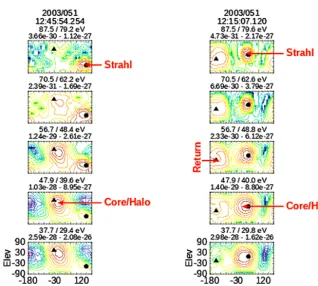
Examples of the plot format are illustrated in Fig. 2, which shows two columns of five φ–θ plots. Both columns show
only a subset of the energy steps being returned. The start-ing time of the spin of data used in the plots is shown at the top of each column. The left-hand column of plots is a se-quential set of cuts in energy through the solar wind eVDF. The energy range shown contains the upper-energy edge of the core/halo and the lower-energy edge of the strahl. The core and halo populations always overlap in aφ–θ plot and cannot be separated. They are treated as a single population called the core/halo and are centered in the plot and move anti-sunward. Because the strahl is field-aligned, it will al-ways be centered on one of the two magnetic field points (in this case the head). Note that while the core/halo and strahl overlap in energy they are, in this example, fully separable in angle because there is a significant nonradial component of the magnetic field that shifts the strahl off the core/halo. The angular separation allows the two populations to be masked off and then integrated to provide for two separate sets of moments, one for the core/halo and one for the strahl.
The right-hand column of φ–θ plots is derived from a typical foreshock eVDF and shows characteristics similar to what is seen in the first column of plots with the exception that it contains a population of return electrons centered on the magnetic field tail projection point (moving sunward). These electrons are either solar wind electrons that have been scattered off the bow shock or electrons that have leaked through the bow shock from the magnetosheath. This popu-lation is present anytime a spacecraft is in the foreshock (Lar-son et al., 1996) and can be used to determine if the space-craft is interior or exterior to the foreshock. It generally has a much higher thermal energy than does the strahl.
Whileφ–θplots are extremely useful in looking at details of the eVDF, there are certain caveats one needs to keep in mind. These caveats arise both from the map projection used in displaying the data and from various preprocessing algo-rithms and will be briefly touched on below. First and fore-most, however, one should recognize that the primary pur-pose of this plot format as applied to this paper is to highlight features of the eVDF that are relevant to the objectives of this analysis.
Map projection format. The plots in Fig. 2 are shown
Figure 2.φ–θplots from the solar wind (left) and the foreshock (right). The solar wind consists of a core, halo, and strahl population. The core/halo appear as a single population in the plots, but because of the energy range covered, it is probably primarily the halo that is seen. The foreshock is identical to the solar wind but includes a set of return electrons that are moving back upstream.
is possible to plot the φ–θ plots in a large number of mapping projections. The left column of plots in Fig. 3 shows the identical set of plots in the right-hand col-umn in Fig. 2 but plotted using a cylindrical equidis-tance mapping projection.
Magnetic field projection points. Variations in the
mag-netic field within the time covered by a 3-D eVDF can affect the position of the projection points with respect to features in the eVDF, leading to possible confusion. For this reason the magnetic field used generally has a higher temporal resolution than the eVDF. The mag-netic field vectors accumulated within the time interval associated with the 3-D eVDF can either be simple av-erages with the averaged values used to form the pro-jection points, or all of the project points formed from the individual magnetic field vectors can be shown in the φ–θ plots. The first usage allows for a very exact estimation of the magnetic field within the time covered by aφ–θplot while the latter (shown in the right-hand column of plots in Fig. 3) is often used when it is sus-pected that the magnetic field has significant variation within the plot time. In this case (from the figure) the magnetic field is seen to have enough jitter to broaden the two projection points but not enough to significantly
cause any confusion of the location of the projections with respect to strahl.
Smoothing. It is standard practice when producing φ–θ
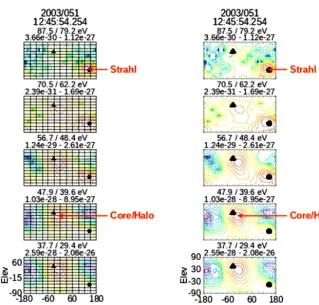
plots to subject the data to a spherical harmonic analy-sis as a means of smoothing the eVDF (Viñas and Gur-giolo, 2009). This in essence artificially increases the total density of data points in the plot. The advantage of using spherical harmonics is that they smooth without creating spurious new features. The left-hand column of plots in Fig. 4 shows the identical plots in the left-hand column of Fig. 2 but with no smoothing and contour-ing turned off. The individual colored grids match the instrument angular resolutions. The plots are definitely coarser than those shown in Fig. 2, but the same fea-tures are seen in both. This is not surprising. Viñas and Gurgiolo (2009) have shown that the plasma moments formed during a spherical harmonics analysis are virtu-ally identical to those formed from the raw data, imply-ing that the fittimply-ing to a set of spherical harmonics has minimal effect on the actual eVDFs.
Scaling. In general individualφ–θplots are autoscaled. To
Figure 3.φ–θplots identical to those on the left in Fig. 2. Here the left-hand column of plots shown is a cylindrical equidistance projection and the right column of plots is shown using the full-resolution magnetic field projection points (about 20 values).
of Fig. 2 but with autoscaling turned off. In this case the scaling used in all plots is given by the color bar at the bottom of the column. Autoscaling is useful when the column of plots spans a large energy range where there is enough fall-off in intensity that features in the high-energy plots are lost due to an insufficient number of contours and/or colors.
As noted above when the magnetic field has a large non-radial component, as in the solar wind example in Fig. 2, the core/halo can be fully separated due to the offset of the strahl from the core/halo. Even when there is a strong radial com-ponent in the field as in the foreshock example in Fig. 2, it is still possible to estimate the approximate transition energy where the plasma is shown in theφ–θplots transitions from primarily strahl to the core/halo even though the two popula-tions cannot be fully separated. Note that near 47.9 eV there is a small but noticeable shift in the overall distribution from a slightly off-radial to a more radial flow. This is the energy at which the core/halo becomes the more dominant population.
4 Observations
Between 2001 and 2012 inclusive, there were over 180 time intervals when the Cluster spacecraft were partially or totally
upstream of the bow shock (in the solar wind and/or fore-shock) and the spacecraft were using burst-mode telemetry. The periods vary between 1.5 to 4 h in length and are gener-ally made up of a mixture of pure solar wind and foreshock plasma. Seventeen of these periods were identified as con-taining definite diffusion signatures. The identifications were made using restrictive criteria that required eVDFs to exhibit both a tongue of electrons that extends from the strahl to-wards the opposite magnetic field projection point and a clear observation of a proto-halo population in one or more energy steps. There were a number of other times during which only a tongue of particles was seen with no distinct proto-halo population. In those cases, either the proto-halo did not form or was too weak to be observed as a clear and distinct particle population within the tongue. These events are not included in this study.
Figure 4.φ–θ plots identical to those on the left in Fig. 2. Here the left-hand column is plotted without any smoothing or fitting and the right column of plots is shown with autoscaling off. In this case all plots have identical scaling according to the color bar at the bottom of the column.
[image:6.612.136.460.396.667.2]Consider the left-hand column of plots in Fig. 2 which show a partial eVDF typical of the pure solar wind containing a core/halo and strahl population. There is no evidence of a tongue at any of the energy steps where both populations are observed. Contrast this with the left-hand column of plots in Fig. 9, which shows a subset of energies from a single eVDF within a region of diffusion. Here the tongue appears to develop, with the emergence of the proto-halo suggesting some connection between the two, which would make sense if the proto-halo is in essence a reformation of the strahl. Still, this cannot be proven conclusively with the data avail-able but maybe with future modeling.
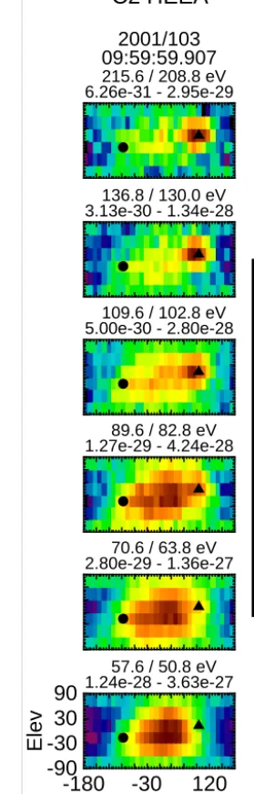
The diffusion signatures in each of the included 17 cases are similar in appearance. The major differences are the en-ergy ranges over which the diffusion was observed and the direction of the tongue, the latter depending on the orien-tation of the magnetic field. Figure 5 contains three exam-ples of diffusion from different times in different years. Each column of plots is a partial representation of a single eVDF. The vertical bar to the right of each column is the energy range in the eVDF that comprises the diffusion zone, extend-ing from the upper energy where the electron tongue first ap-pears down to the energy at which the proto-halo is no longer observable. The energy steps in the first column of plots are contiguous but are not in the next two columns of plots. The φ–θplots at the upper- and lower-energy limits of the diffu-sion zone, however, are included. The three examples detail not only the effect of magnetic field orientation on the dif-fusion (orientation of the tongue) but also variations in the energy range of the diffusion zone. Figure 6 shows the iden-tical set of plots as the right-hand column of Fig. 5 but with both smoothing and contours turned off. The plots in the fig-ure reinforce the claim that smoothing does not significantly alter features in the eVDFs but simply makes them easier to pick out.
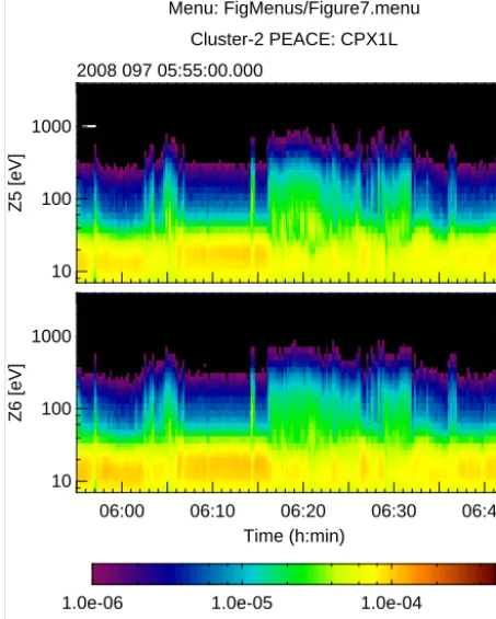
The characteristics associated with diffusion observations are presented and discussed here in the context of a 48 min stretch of data from 6 April 2008 (DOY 97) between 05:55 and 06:43 UT from the Cluster-2 LEEA analyzer, which was returning data in 12 elevation bins, 32 azimuth bins and 30 energy steps covering 7 to 3952 eV. During this time interval the spacecraft was in the vicinity of the bow shock/magnetosheath with multiple transitions into and out of the foreshock and pure solar wind. Diffusion signatures were seen in each solar wind interval. This is a period of fast wind with an average wind speed of over 700 km s−1.
Figure 7 shows a set of spectrograms covering the time period from the two PEACE elevation zones closest to the ecliptic plane. The plot begins at the onset of the burst-mode telemetry and runs until the spacecraft begins making multi-ple short excursions into and out of the magnetosheath. The lines in the top plot indicate times when the spacecraft was in pure solar wind. Those intervals are coincident with no-ticeable depressions in the intensity of the>80 eV electron fluxes that result from the absence of return electrons. This
C2 HEEA
6.26e-31 - 2.95e-29 215.6 / 208.8 eV
09:59:59.907 2001/103
● ▲
3.13e-30 - 1.34e-28 136.8 / 130.0 eV
● ▲
5.00e-30 - 2.80e-28 109.6 / 102.8 eV
● ▲
1.27e-29 - 4.24e-28 89.6 / 82.8 eV
● ▲
2.80e-29 - 1.36e-27 70.6 / 63.8 eV
● ▲
-180
-30
120
Phase
-90
-30
30
90
Elev
1.24e-28 - 3.63e-27 57.6 / 50.8 eV
● ▲
[image:7.612.355.495.77.513.2]Diffusion region
Figure 6.Fiveφ–θplots identical to the right-most column of plots in Fig. 5 with no smoothing or contouring. The figure reinforces the claim that smoothing neither alters nor adds any features that exist in the eVDF. The tongue and proto-halo are both clearly seen in the plots.
10 100 1000
06:00 06:10 06:20 06:30 06:40
Time (h:min)
10 100 1000
1.0e-06 1.0e-05 1.0e-04
2008 097 05:55:00.000
Z5 [eV]
Z6 [eV]
[image:8.612.53.280.70.353.2]Differential energy flux Cluster-2 PEACE: CPX1L Menu: FigMenus/Figure7.menu
Figure 7.Spectrograms of the PEACE elevation zones above and below the ecliptic plane. The interval shown includes multiple ex-cursions into and out of the solar wind and foreshock. Arrows show depressions in the intensity, which are intervals where the spacecraft was in the solar wind and in the presence of diffusion. The intensity depressions are the result of the absence of return electrons.
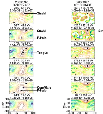
[image:8.612.313.540.87.485.2]The observed diffusion during this time period is consis-tent and strong. A good picture of its features is seen in Fig. 9. Shown are two sets of φ–θ plots generated from a single eVDF observed in a diffusion event. The left set of plots shows a contiguous set of energies covering the diffu-sion zone (∼56.7 down to∼30.1 eV). The right set of plots shows energies above the diffusion zone with the lower two energy steps being contiguous with those in the left-hand set of plots. Above that every other energy step is shown. Fea-tures of interest are indicated by arrows and labels. At 70 eV and above one sees only the strahl population, which extends up to 584 eV (an energy step not included in the figure). The φ–θplot at 669 eV is basically noise that appears significant only because of the autoscaling of the plot intensity. The for-mation of the tongue begins at about 56.7 eV and extends downward in energy to just about where the core/halo be-gins to emerge in the plots. At these energies both the proto-halo and strahl (where it exists) are embedded in the tongue. By 37.7 eV the strahl has weakened to the point where it is only minimally present. There also might be a minimal manifestation of the core/halo present at this energy; how-ever, by 30.1 eV there is a strong core/halo population
signa-3.0 3.5 4.0 4.5 5.0
10 12 14 16 18
540 630 720 810 900
4 5 6 7 8
72 144 216 288 360
06:00 06:12 06:24 06:36 Time (h:min)
-90 -54 -18 18 54 90
2008 097 05:55:00.000
C2 LEEA MF & moments
N [/cc]
T [eV]
V [km s ]
B [nT]
BΦ
[deg]
B
[deg]
-1
Figure 8.Plots of the total electron density, temperature, and speed and magnetic field components across the time interval in Fig. 7. The baseline temperatures occur when the spacecraft is in the solar wind. The inclusion of the higher temperature return population in the foreshock results in an increase in temperature above the base-line.
ture together with a proto-halo. Finally, at 24.3 eV only the core/halo population exists. It is reasonable to assume that the strahl covers the same energy range here as it would if there were no diffusion present; that is, the low-energy por-tion of the strahl is intact and has undergone no, or only min-imal, diffusion. We will look at this in more depth when we discuss the density spectra within the diffusion region shown in Fig. 12.
dif-Figure 9.A set ofφ–θplots showing the formation of the tongue of electrons and the proto-halo as a function of energy. The left column shows continuous energy steps bracketing the diffusion, while the right column shows energies above the diffusion energy range. The two lowest energy steps in the right panel are a continuation of those in the left panel, while the remaining show every other energy step.
fusion zone the strahl shifts off the magnetic field. This shift is seen in almost every examined time period in which diffu-sion is present, but it is not seen, at least to the same extent, if at all, either in the solar wind in the absence of diffusion or in the foreshock. The second feature to note is the clear ellip-tical appearance of the strahl in and near the diffusion zone rather than the expected more circular appearance as seen in the foreshock eVDF in the right column of plots in Fig. 2. Both of these features seem to be unique to the diffusion pro-cess and may be the result of the mechanisms driving it.
Because the proto-halo and strahl are well separated in velocity space within this time period, it is possible within the energy steps where both populations exist to define ve-locity space volumes that individually isolate the two pop-ulations. Integrating over the volumes provides estimates of the density and velocity in each population. An example is shown in Fig. 10 for multiple eVDFs between 06:10:20 and
[image:9.612.128.466.67.441.2]2008 097 (47.9 eV)
•••• • ••••• • • • • • • • • • • • • • • • • • • • • • • • • • • • • • • • • • • • • • • • • • • • • • • • • • • • • • • • • • • • • • • • • • • • • • • • • • • • • • • • • • • • • • • • • • • • • • • • • • • • • • • • • • • • • • • • • • • • • • • • • • • • • • • • • • • • • • • • • • • • • • • • • • • • • • • • • • • • • • • • • • • • • • • • • • • • • • • • • • • • • • • • ••••••••• •••••••••••••• • • • • • • • • • • • • • • • • • • • • • • • • • • • • • • • • • • • • • • • • • • • • • • • • • • • • • • • • • • • • • • • • • • • • • • • • • • • • • • • • • • • • • • • • • • • • • • • • • • • • • • • • • • • • • • • • • • • • • • • • • • • • • • • • • • • • • • • • • • • • • • • • • • • • • • • • • • • • • • • • • • • • • • • • • • • • • • • • • • • • • • • • • • • • • • • • • • • • • • • • • • • • • • • • • • • • • • • • • • • • • • • • • • • • • • • • • • • • • • • • • • • • • • • • • • • • • • • ••••••••••••• •••••••••••••••••• • • • • • • • • • • • • • • • • • • • • • • • • • • • • • • • • • • • • • • • • • • • • • • • • • • • • • • • • • • • • • • • • • • • • • • • • • • • • • • • • • • • • • • • • • • • • • • • • • • • • • • • • • • • • • • • • • • • • • • • • • • • • • • • • • •••••••••••••••3.54e-29 - 3.03e-27 47.9 / 40.6 eV 06:10:19.437 ● ▲ •••• • ••••• • • • • • • • • • • • • • • • • • • • • • • • • • • • • • • • • • • • • • • • • • • • • • • • • • • • • • • • • • • • • • • • • • • • • • • • • • • • • • • • • • • • • • • • • • • • • • • • • • • • • • • • • • • • • • • • • • • • • • • • • • • • • • • • • • • • • • • • • • • • • • • • • • • • • • • • • • • • • • • • • • • • • • • • • • • • • • • • • • • • • • • • ••••••••• •••••••••••• • • • • • • • • • • • • • • • • • • • • • • • • • • • • • • • • • • • • • • • • • • • • • • • • • • • • • • • • • • • • • • • • • • • • • • • • • • • • • • • • • • • • • • • • • • • • • • • • • • • • • • • • • • • • • • • • • • • • • • • • • • • • • • • • • • • • • • • • • • • • • • • • • • • • • • • • • • • • • • • • • • • • • • • • • • • • • • • • • • • • • • • • • • • • • • • • • • • • • • • • • • • • • • • • • • • • • • • • • • • • • • • • • • • • • • • • • • • • • • • • • • • • • • • • • • • • • • • • • ••••••••••••• •••••••••••••••• • • • • • • • • • • • • • • • • • • • • • • • • • • • • • • • • • • • • • • • • • • • • • • • • • • • • • • • • • • • • • • • • • • • • • • • • • • • • • • • • • • • • • • • • • • • • • • • • • • • • • • • • • • • • • • • • • • • • • • • • • • • • • • • • • • • •••••••••••••••
3.63e-30 - 3.04e-27 47.9 / 40.6 eV 06:10:27.717 ● ▲ •••• • ••••• • • • • • • • • • • • • • • • • • • • • • • • • • • • • • • • • • • • • • • • • • • • • • • • • • • • • • • • • • • • • • • • • • • • • • • • • • • • • • • • • • • • • • • • • • • • • • • • • • • • • • • • • • • • • • • • • • • • • • • • • • • • • • • • • • • • • • • • • • • • • • • • • • • • • • • • • • • • • • • • • • • • • • • • • • • • • • • • • • • • • • • • ••••••••• •••••••••••••• • • • • • • • • • • • • • • • • • • • • • • • • • • • • • • • • • • • • • • • • • • • • • • • • • • • • • • • • • • • • • • • • • • • • • • • • • • • • • • • • • • • • • • • • • • • • • • • • • • • • • • • • • • • • • • • • • • • • • • • • • • • • • • • • • • • • • • • • • • • • • • • • • • • • • • • • • • • • • • • • • • • • • • • • • • • • • • • • • • • • • • • • • • • • • • • • • • • • • • • • • • • • • • • • • • • • • • • • • • • • • • • • • • • • • • • • • • • • • • • • • • • • • • • • • • • • • • • • • • • ••••••••• •••••••••••••••••• • • • • • • • • • • • • • • • • • • • • • • • • • • • • • • • • • • • • • • • • • • • • • • • • • • • • • • • • • • • • • • • • • • • • • • • • • • • • • • • • • • • • • • • • • • • • • • • • • • • • • • • • • • • • • • • • • • • • • • • • • • • • • • • • • •••••••••••••••
2.66e-29 - 3.27e-27 47.9 / 40.6 eV06:10:35.993
● ▲ •••• • ••••• • • • • • • • • • • • • • • • • • • • • • • • • • • • • • • • • • • • • • • • • • • • • • • • • • • • • • • • • • • • • • • • • • • • • • • • • • • • • • • • • • • • • • • • • • • • • • • • • • • • • • • • • • • • • • • • • • • • • • • • • • • • • • • • • • • • • • • • • • • • • • • • • • • • • • • • • • • • • • • • • • • • • • • • • • • • • • • • • • • • • • • • ••••••••• •••••••••••• • • • • • • • • • • • • • • • • • • • • • • • • • • • • • • • • • • • • • • • • • • • • • • • • • • • • • • • • • • • • • • • • • • • • • • • • • • • • • • • • • • • • • • • • • • • • • • • • • • • • • • • • • • • • • • • • • • • • • • • • • • • • • • • • • • • • • • • • • • • • • • • • • • • • • • • • • • • • • • • • • • • • • • • • • • • • • • • • • • • • • • • • • • • • • • • • • • • • • • • • • • • • • • • • • • • • • • • • • • • • • • • • • • • • • • • • • • • • • • • • • • • • • • • • • • • • • • • • • ••••••••••••• •••••••••••••••• • • • • • • • • • • • • • • • • • • • • • • • • • • • • • • • • • • • • • • • • • • • • • • • • • • • • • • • • • • • • • • • • • • • • • • • • • • • • • • • • • • • • • • • • • • • • • • • • • • • • • • • • • • • • • • • • • • • • • • • • • • • • • • • • • • • •••••••••••••••
6.45e-30 - 3.20e-27 47.9 / 40.6 eV 06:10:44.268 ● ▲ •••• • ••••• • • • • • • • • • • • • • • • • • • • • • • • • • • • • • • • • • • • • • • • • • • • • • • • • • • • • • • • • • • • • • • • • • • • • • • • • • • • • • • • • • • • • • • • • • • • • • • • • • • • • • • • • • • • • • • • • • • • • • • • • • • • • • • • • • • • • • • • • • • • • • • • • • • • • • • • • • • • • • • • • • • • • • • • • • • • • • • • • • • • • • • • ••••••••• •••••••••••••• • • • • • • • • • • • • • • • • • • • • • • • • • • • • • • • • • • • • • • • • • • • • • • • • • • • • • • • • • • • • • • • • • • • • • • • • • • • • • • • • • • • • • • • • • • • • • • • • • • • • • • • • • • • • • • • • • • • • • • • • • • • • • • • • • • • • • • • • • • • • • • • • • • • • • • • • • • • • • • • • • • • • • • • • • • • • • • • • • • • • • • • • • • • • • • • • • • • • • • • • • • • • • • • • • • • • • • • • • • • • • • • • • • • • • • • • • • • • • • • • • • • • • • • • • • • • • • • • • • • ••••••••• ••••••• • • ••••••••• • • • • • • • • • • • • • • • • • • • • • • • • • • • • • • • • • • • • • • • • • • • • • • • • • • • • • • • • • • • • • • • • • • • • • • • • • • • • • • • • • • • • • • • • • • • • • • • • • • • • • • • • • • • • • • • • • • • • • • • • • • • • • • • • • •••••••••••••••
-180 -60 60 180
Phase -90 -30 30 90 Elev
1.60e-29 - 2.91e-27 47.9 / 40.6 eV06:10:52.546
●
▲
Strahl
P-Halo
Tongue
Figure 10.Fiveφ–θplots of the 47.9 eV energy channel taken from different eVDFs within the time frame covered in Fig. 11 showing the volumes used to estimate the strahl, proto-halo, and tongue mo-ments.
the individual population densities, but also any density ex-terior to the defined volumes. The normalized velocity is the contribution to the total velocity by a given population and is defined as
VP ,n,i=
NP NF
VP ,i, (1)
where the subscriptirepresents the velocity components (x, y,z),P is the population, andNFis the full electron density. The features seen in Fig. 11 are common to all the diffu-sion events looked at so far. The tongue contributes very little to either the density or to the total velocity. Both the strahl and proto-halo are moving basically anti-sunward (GSE Vx components are negative). TheVyandVzcomponents,
how-0.000 0.015 0.030 0.045 0.060 0.075 0 400 800 1200 1600 2000 -2000 -1500 -1000-500 0 500 -400 -2000 200 400 600
08:00 09:00 10:00 11:00 12:00
Time (min:s) -600 -3000 300 600 900
2008 097 06:08:00.000
C2 LEEA moments (48 eV)
V z [ k m s ] V y [ k m s ]
Vx [km s ]
V [km s ]
N [/cc] Full Strahl P-Halo Tongue -1 -1 -1 -1
Figure 11.Electron plasma density, speed, and velocity (top to bot-tom) computed from the 48 eV energy channel. The moments are computed over the entire energy step (black), within the volume defining the proto-halo (red) and within the volume defining the strahl (blue).
ever, have close to opposite flows so that both the totalVy andVzvelocities are close to 0. This is true more forVzand Vy. Basically, the overall flow at this energy step is approxi-mately radial with an average energy in this energy channel ∼7.3 eV, well below the measurement energy. Individually the average energy of each population is about 40 eV, consis-tent with the poconsis-tential reduced measurement energy.
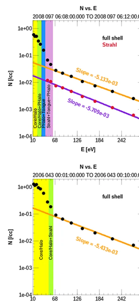
popu-lation (cf. the 37.7 eV energy step in Fig. 9). The orange and purple lines are fits to the data above 60 eV for the full and strahl densities spectra, respectively. The difference in the in-tensity between the strahl and full-density spectra is due to the inclusion of the electrons outside the defined strahl veloc-ity space volume. The shaded areas at the left in both plots show the mixture of populations present in theφ–θplots. The diffusion zone is defined by the combined green, blue, and purple shadings in the top plot. This is a good picture of the general progression of electron populations within the diffu-sion zone and representative of the events we have looked at.
The top and bottom spectral plots are very similar in shape; this is despite the presence (absence) of diffusion in the up-per (lower) plot, something to consider when using fits to model distributions to estimate the characteristics of the elec-tron populations. Note that the data used to construct the bot-tom plot were taken approximately 2 years prior to the data used in the upper plot, so there should be no expectation for the spectral intensity in the two spectra to be comparable. Both full-density spectral plots show a break at 60 eV. In the top plot this corresponds to the energy where the tongue and proto-halo are first seen and in the bottom plot where the core/halo is first seen. The fact that there is no corresponding break in the strahl density spectrum suggests that the strahl plays no role in the break in the full-density spectrum.
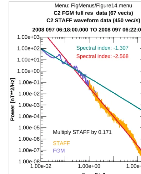
[image:11.612.313.540.101.596.2]We have also looked at the magnetic field spectral power in the absence and presence of diffusion. Two examples are shown in Fig. 13, taken during the times represented by the two density spectra in Fig. 12. Both are from pure solar wind, but the upper spectrum is from the time during which there was active diffusion and the lower from the time with no dif-fusion. Each spectrum is a combination of spectra built from the full-resolution FGM data (blue portion of the total spec-trum) and the STAFF waveform data (orange portion of the spectrum), and both are normalized using their overlap be-tween 1 and 2 Hz. The two spectra are very similar in the STAFF frequency range but show significant differences in the FGM portion. The FGM portion of the spectra is gener-ally very dynamic even within adjoining time intervals. This carries through to the majority of the spectra generated in conjunction with this study. Both spectra are also very differ-ent from the typical spectra seen in the foreshock, an example of which is shown in Fig. 14. Foreshock spectra are overall flatter and tend to show broadband intensity enhancements in the STAFF portion of the spectrum (between 10 and 100 Hz in this figure). These enhancements are more than likely ev-idence of whistler or other broadband turbulence driven by the free energy in the counterstreaming return and strahl elec-tron populations in the foreshock. It is interesting to note that there are generally no corresponding enhancements seen in the spectra during diffusion events, which probably precludes broadband turbulence as a source of the diffusion.
Figure 13.Magnetic field power density spectra during the two time periods used to form theN vs.Eplots in Fig. 12. The spectra are formed from spectra using the full-resolution FGM data (blue por-tion of the spectra) and the STAFF waveform data (orange porpor-tion of the spectra). The two spectra are normalized between 1 and 2 Hz.
5 Discussion
Of the more than 180 intervals looked at when the Cluster spacecraft were upstream of the bow shock and returning data in burst-mode telemetry, almost 10 % exhibit diffusion signatures that fit the restrictive definition given at the start
1.00e-02 1.00e+00 1.00e+02 1.00e-08
1.00e-07 1.00e-06 1.00e-05 1.00e-04 1.00e-03 1.00e-02 1.00e-01 1.00e+00 1.00e+01 1.00e+02 1.00e+03
2008 097 06:18:00.000 TO 2008 097 06:22:00.000 C2 FGM full res data (67 vec/s) C2 STAFF waveform data (450 vec/s)
Freq [Hz]
Power [nT**2/Hz]
Menu: FigMenus/Figure14.menu
Spectral index: -1.307 Spectral index: -2.568
FGM STAFF
[image:12.612.309.535.66.343.2]Multiply STAFF by 0.171
Figure 14.Spectra of the magnetic field power density from a time when the spacecraft were in the foreshock in Fig. 7. This can be compared to the spectra in Fig. 13.
of Sect. 4. If we use a relaxed definition, requiring only the presence of a definite tongue that extends beyond the nom-inal position of the core/halo, the number of diffusion ob-servations increases to more than 18 % (25 % if we do not include events that are all foreshock).
1.78e-30 - 8.55e-28 87.5 / 80.3 eV
06:16:02.894 2008/097
●
▲
3.67e-31 - 1.30e-27 70.5 / 63.3 eV
●
▲
7.39e-30 - 2.36e-27 56.7 / 49.5 eV
●
▲
9.48e-30 - 3.52e-27 47.9 / 40.7 eV
●
▲
2.84e-29 - 7.85e-27 37.7 / 30.5 eV
●
▲
2.85e-29 - 1.94e-26 30.1 / 22.9 eV
●
▲
-180 -30 120
Phase -90
-30 30 90
Elev
4.60e-28 - 4.38e-26 24.3 / 17.1 eV
●
▲
5.53e-31 - 7.78e-28 87.5 / 80.3 eV
06:16:11.170 2008/097
●
▲
4.59e-30 - 1.35e-27 70.5 / 63.3 eV
●
▲
1.28e-29 - 2.09e-27 56.7 / 49.5 eV
●
▲
9.73e-30 - 3.93e-27 47.9 / 40.7 eV
●
▲
1.38e-29 - 7.16e-27 37.7 / 30.5 eV
●
▲
8.07e-29 - 1.97e-26 30.1 / 22.9 eV
●
▲
-180 -30 120
Phase
4.05e-28 - 4.50e-26 24.3 / 17.1 eV
●
▲
4.50e-31 - 8.37e-28 87.5 / 80.3 eV
06:16:19.446 2008/097
●
▲
4.12e-31 - 1.87e-27 70.5 / 63.3 eV
●
▲
4.63e-31 - 2.56e-27 56.7 / 49.5 eV
●
▲
1.37e-31 - 4.19e-27 47.9 / 40.7 eV
●
▲
1.42e-31 - 8.74e-27 37.7 / 30.5 eV
●
▲
8.20e-29 - 2.24e-26 30.1 / 22.9 eV
●
▲
-180 -30 120
Phase
1.13e-27 - 4.43e-26 24.3 / 17.1 eV
●
▲
3.93e-31 - 9.68e-28 87.5 / 80.3 eV
06:16:27.722 2008/097
●
▲
2.30e-31 - 1.87e-27 70.5 / 63.3 eV
●
▲
1.45e-30 - 3.47e-27 56.7 / 49.5 eV
●
▲
1.03e-29 - 4.34e-27 47.9 / 40.7 eV
●
▲
8.96e-29 - 9.68e-27 37.7 / 30.5 eV
●
▲
1.30e-28 - 2.36e-26 30.1 / 22.9 eV
●
▲
-180 -30 120
Phase
1.36e-27 - 4.89e-26 24.3 / 17.1 eV
●
[image:13.612.133.469.65.481.2]▲
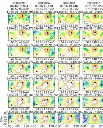
Figure 15.Set of four columns ofφ–θplots showing every other eVDF on a traversal from a region of diffusion (first two columns) into the foreshock (last two columns).
this is at the present unknown. The diffusion results in the creation of two populations of electrons within a confined energy range which we call the diffusion zone. There is cur-rently no evidence that the strahl contributes to either popu-lation, but if it does, it is a minimal contribution. Within the upper energies of the diffusion range, there is no observed core/halo population. It is not inconceivable that at these en-ergies the proto-halo represents the bulk of the core/halo pop-ulation but shifted off the nominal core/halo radial flow lo-cation. The fluid flow in these energy steps is still primarily radial and not that different from what would be expected in the absence of diffusion.
One of the most puzzling observations is the total lack of observations of diffusion signatures anywhere inside the foreshock except in the immediate foreshock/solar wind
over-lap of the two populations similar to that seen in the previous two columns of plots. In the last column, the eVDF exhibits pretty much the standard foreshock characteristics: strahl and return electrons at the upper energies and the core/halo at the lower energies.
The electrons within the diffusion zone are not in a sta-ble configuration. External forces are required to create and maintain the drifts necessary to keep the proto-halo and tongue in the configuration they are observed to have in the diffusion zone. Turning off these forces will allow the dif-fusion populations to relax back into a stable configuration presumably close to what initially existed within the diffu-sion. The minimal penetration of the diffusion populations into the foreshock suggests that the plasma relaxes on a very short timescale back into or close to its pre-diffusion state. This would explain the absence of diffusion signatures inte-rior to the foreshock/solar wind interface and may provide a look at how the diffusion alters the post-diffusion plasma populations.
6 Conclusions
The existence of a diffusion signature in the solar wind eVDF near 1 AU appears to be both common and significant. The diffusion manifests itself in the appearance of two new parti-cle populations within a reasonably narrow energy range: the proto-halo and tongue. Both populations seem to be formed as a result of diffusion in the high-energy portion of the core/halo. Any contribution to their formation from the strahl appears to be minimal.
7 Data availability
With the exception of PEACE data, which were ob-tained from the Mullard Space Science Laboratory (MSSL) science data archive (http://www.mssl.ucl.ac.uk/missions/ cluster/about_peace_data.php), all data were obtained from the Cluster Science Archive (CSA, http://www.cosmos.esa. int/web/csa).
Acknowledgements. The authors would like to acknowledge the work and role of the Cluster Science Archive (CSA) and thank the EFW and FGM teams for providing the data used in this study. We would also like to acknowledge the PEACE team at MSSL who worked on and are constantly improving the instrument calibration. Both of us would like to acknowledge support from NASA Grant NNX15AI88G.
The topical editor, M. Temmer, thanks three anonymous refer-ees for help in evaluating this paper.
References
Balogh, A., Dunlop, M. W., Cowley, S. W. H., Southwood, D. J., Thomlinson, J. G., Glassmeier, K. H., Musmann, G., Luhr, H., Buchert, S., Acuna, M. H., Fairfield, D. H., Slavin, J. A., Riedler, W., Schwingenschuh, K., and Kivelson, M. G.: The Cluster Magnetic Field Investigation, Space Sci. Rev., 79, 65– 91, doi:10.1023/A:1004970907748, 1997.
Che, H. and Goldstein, M. L.: The Origin of Non-Maxwellian So-lar Wind Electron Velocity Distribution Function: Connection to Nanoflares in the Solar Corona, Astrophys. J. Lett., 795, L38, doi:10.1088/2041-8205/795/2/L38, 2014.
Che, H., Goldstein, M. L., and Viñas, A. F.: Bidirectional en-ergy cascades and the origin of kinetic Alfvénic and whistler turbulence in the solar wind., Phys. Rev. Lett., 112, 061101, doi:10.1103/PhysRevLett.112.061101, 2014.
Cornilleau-Wehrlin, N., Chauveau, P., Louis, S., Meyer, A., Nappa, J. M., Perraut, S., Rezeau, L., Robert, P., Roux, A., de Villedary, C., de Conchy, Y., Friel, L., Harvey, C. C., Hubert, D., Lacombe, C., Manning, R., Wouters, F., Lefeuvre, F., Parrot, M., Pincon, J. L., Poirier, B., Kofman, W., and Louarn, P.: The Cluster Spatio-Temporal Analysis of Field Fluctuations (STAFF) Experiment, Space Sci. Rev., 79, 107–136, doi:10.1023/A:1004979209565, 1997.
Cornilleau-Wehrlin, N., Mirioni, L., Robert, P., Bouzid, V., Mak-simovic, M., de Conchy, Y., Harvey, C. C., and Santolík, O.: STAFF Instrument Products Distributed Through the Cluster Active Archive, in: The Cluster Active Archive, Studying the Earth’s Space Plasma Environment, edited by: Laakso, H., Tay-lor, M. G. T. T., and Escoubet, C. P., Proceedings of As-trophysics and Space Science, Springer, Berlin, 11, 159–168, doi:10.1007/978-90-481-3499-1_10, 2010.
Dum, C. T., Marsch, E., and Pilipp, W.: Determina-tion of wave growth from measured distribuDetermina-tion func-tions and transport theory, J. Plasma Phys., 23, 91–113, doi:10.1017/S0022377800022170, 1980.
Fazakerley, A. N., Lahiff, A. D., Wilson, R. J., Rozum, I., Anekallu, C., West, M., and Bacai, H.: PEACE Data in the Cluster Active Archive, in: The Cluster Active Archive, Studying the Earth’s Space Plasma Environment, edited by: Laakso, H., Taylor, M. G. T. T., and Escoubet, C. P., Proceedings of Astrophysics and Space Science, Springer, Berlin, 11, 129–144, doi:10.1007/978-90-481-3499-1_8, 2010.
Feldman, W. C., Asbridge, J. R., Bame, S. J., Montgomery, M. D., and Gary, S. P.: Solar wind electrons, J. Geophys. Res., 80, 4181– 4196, 1975.
Gary, S. P. and Saito, S.: Broadening of solar wind strahl pitch-angles by the electron/electron instability: Particle-in-cell simulations, Geophys. Res. Lett., 34, L14111, doi:10.1029/2007GL030039, 2007.
Gary, S. P., Saito, S., and Li, H.: Cascade of whistler turbulence: Particle-in-cell simulations, Geophys. Res. Lett., 35, L02104, doi:10.1029/2007GL032327, 2008.
Gurgiolo, C., Goldstein, M. L., Viñas, A. F., and Fazakerley, A. N.: Direct observations of the formation of the solar wind halo from the strahl, Ann. Geophys., 30, 163–175, doi:10.5194/angeo-30-163-2012, 2012.
Gustafsson, G., Bostrom, R., Holback, B., Holmgren, G., Lundgren, A., Stasiewicz, K., Ahlen, L., Mozer, F. S., Pankow, D., Harvey, P., Berg, P., Ulrich, R., Pedersen, A., Schmidt, R., Butler, A., Fransen, A. W. C., Klinge, D., Thomsen, M., Falthammar, C.-G., Lindqvist, P.-A., Christenson, S., Holtet, J., Lybekk, B., Sten, T. A., Tanskanen, P., Lappalainen, K., and Wygant, J.: The Elec-tric Field and Wave Experiment for the Cluster Mission, Space Sci. Rev., 79, 137–156, doi:10.1023/A:1004975108657, 1997. Hammond, C. M., Feldman, W. C., McComas, D. J., and Forsyth,
R. J.: Variation of electron-strahl width in the high-speed so-lar wind : ULYSSES observations, Astron. Astrophys., 316, 350– 354, 1996.
Johnstone, A. D., Alsop, C., Gurge, S., Carter, P. J., Coates, A. J., Coker, A. J., Fazakerley, A. N., Grande, M., Gowen, R. A., Gur-giolo, C., Hancock, B. K., Narheim, B., Preece, A., Sheather, P. H., Winningham, J. D., and Woodcliffe, R. D.: PEACE: A plasma electron and current experiment, Space Sci. Rev., 79, 351–398, 1997.
Khotyaintsev, Y., Lindqvist, P.-A., Eriksson, A., and André, M.: The EFW Data in the CAA, in: The Cluster Active Archive, Study-ing the Earth’s Space Plasma Environment, edited by: Laakso, H., Taylor, M. G. T. T., and Escoubet, C. P., Proceedings of Astrophysics and Space Science, Springer, Berlin, 11, 97–108, doi:10.1007/978-90-481-3499-1_6, 2010.
Landi, S., Matteini, L., and Pantellini, F.: On the Competi-tion Between Radial Expansion and Coulomb Collisions in Shaping the Electron Velocity Distribution Function: Kinetic Simulations, Astrophys. J. Lett., 760, 143, doi:10.1088/0004-637X/760/2/143, 2012.
Larson, D. E., Lin, R. P., McFadden, J. P., Ergun, R. E., Carlson, C. W., Anderson, K. A., Phan, T. D., McCarthy, M. P., Parks, G. K., Rème, H., Bosqued, J. M., d’Uston, C., Sanderson, T. R., Wenzel, K. P., and Lepping, R. P.: Probing the Earth’s bow shock with upstream electrons, Geophys. Res. Lett., 23, 2203–2206, doi:10.1029/96GL02382, 1996.
Lin, R. P.: Wind observations of suprathermal electrons in the inter-planetary medium, Space Sci. Rev., 86, 61–78, 1998.
Maksimovic, M., Zouganelis, I., Chaufray, J.-Y., Issautier, K., Scime, E. E., Littleton, J. E., Marsch, E., McComas, D. J., Salem, C., Lin, R. P., and Elliott, H.: Radial evolution of the electron dis-tribution functions in the fast solar wind between 0.3 and 1.5 AU, J. Geophys. Res.-Space, 110, 9104, doi:10.1029/2005JA011119, 2005.
Owens, M. J., Crooker, N. U., and Schwadron, N. A.: Suprathermal electron evolution in a Parker spiral magnetic field, J. Geophys. Res., 113, A11104, doi:10.1029/2008JA013294, 2008.
Pavan, J., Viñas, A. F., Yoon, P. H., Ziebell, L. F., and Gaelzer, R.: Solar Wind Strahl Broadening by Self-generated Plasma Waves, Astrophys. J. Lett., 769, L30, doi:10.1088/2041-8205/769/2/L30, 2013.
Pierrard, V., Lazar, M., and Schlickeiser, R.: Evolution of the elec-tric distribution function in whistler wave turbulence of the solar wind, Sol. Phys., 269, 421–438, doi:10.1007/s11207-010-9700-7, 2011.
Pilipp, W. G., Miggenrieder, H., Montgomery, M. D., Mühlhaüser, K. H., Rosenbauer, H., and Schwenn, R.: Characteristics of elec-tron velocity distribution functions in the solar wind derived from Helios Plasma Experiment, J. Geophys. Res., 92, 1075–1092, 1987a.
Pilipp, W. G., Miggenrieder, H., Mühlhaüser, K. H., Rosenbauer, H., Schwenn, R., and Neubauer, F. M.: Variations of electron ve-locity distribution functions in the solar wind, J. Geophys. Res., 92, 1103–1118, 1987b.
Rosenbauer, H., Miggenrieder, H., Montgomery, M. D., and Schwenn, R.: Preliminary results of the Helios plasma experi-ment, in: Physics of Solar Planetary Environments, edited by: Williams, D. J., American Geophysical Union, Washington DC, USA, p. 319, 1976.
Rosenbauer, H., Schwenn, R., Marsch, E., Meyer, B., H, M., Mont-gomery, M. D., Muhlhausser, K. H., Pilipp, W., Voges, W., and Zink, S. M.: A survey on initial results of the Helios plasma ex-periment, J. Geophys., 42, 561–580, 1977.
Saito, S. and Gary, S. P.: Whistler scattering of suprathermal elec-trons in the solar wind: Particle-in-cell simulations, J. Geophys. Res., 112, A06116, doi:10.1029/2006JA012216, 2007a. Saito, S. and Gary, S. P.: All whistlers are not created
equally: Scattering of strahl electrons in the solar wind via particle-in-cell simulations, Geophys. Res. Lett., 34, L01102, doi:10.1029/2006GL028173, 2007b.
Seough, J., Nariyuki, Y., Yoon, P. H., and Saito, S.: Strahl Formation in the Solar Wind Electrons via Whistler Instability, Astrophys. J. Lett., 811, L7, doi:10.1088/2041-8205/811/1/L7, 2015. Stverák, v. S. v., Maksimovic, M., Trávníˇceik, P., Marsch, E.,
Faza-kerley, A. N., and Scieme, E. E.: Radial evolution of nonther-mal electron populations in the low-latitude solar wind: Clus-ter and Ulysses observations, J. Geophys. Res., 114, A05104, doi:10.1029/2008JA013883, 2009.
Viñas, A. F. and Gurgiolo, C.: Spherical harmonic analysis of par-ticle velocity distribution function: Comparison of moments and anisotropies using Cluster data, J. Geophys. Res., 114, A01105, doi:10.1029/2008JA013633, 2009.
Viñas, A. F., Gurgiolo, C., Nieves-Chinchilla, T., Gary, S. P., and Goldstein, M. L.: Whistler waves driven by anisotropic 3D strahl velocity distributions in the solar wind: Cluster observations, in: AIP Proceedings of Solar Wind 12 Conference, edited by: Mak-simovic, M., Issautier, K., Meyer-Vernet, N., Moncuquet, M., and Pantellini, F., American Institute of Physics, New York, NY, USA, p. 265, 2010.
Vocks, C.: Kinetic Models for Whistler Wave Scattering of Elec-trons in the Solar Corona and Wind, Space Sci. Rev., 172, 303– 314, doi:10.1007/s11214-011-9749-0, 2012.
Vocks, C., Lin, R. P., and Mann, G.: Electron halo and strahl for-mation in the solar wind by resonant interaction with whistler waves, Astrophys. J., 627, 540–549, doi:10.1086/430119, 2005. Vocks, C., Mann, G., and Rausche, G.: Formation of suprathermal
electron distributions in the quiet solar corona, Astron. Astro-phys., 480, 527–536, doi:10.1051/0004-6361:20078826, 2008. Wang, L., Lin, R. P., Salem, C., Pulupa, M., Larson, D. E., Yoon,