Learning and Using Taxonomies for Visual and Olfactory Classification

(1)

Classification

Thesis by

Greg Griffin

In Partial Fulfillment of the Requirements for the Degree of

Doctor of Philosophy

California Institute of Technology Pasadena, California

2013

(2)

c

2013

(3)

(4)

(5)

Acknowledgements

First and foremost I would like to thank my advisor, Dr. Pietro Perona. I simply could not have asked for a kinder advisor or a better learning experience. Without his patient support and imag-ination none of this would have even started. Dr. Nate Lewis and Dr. Richard Flagan have also been extremely gracious in sharing their projects with me. Pietro and Rick have been a constant source of encouragement and brain-storming, and Nate and his students Marc Woodka and Edgardo Garcia-Berrios not only provided extremely sensitive sensors but gave me copious help in an area of research I knew very little about. Finally I would like to give my heartfelt thanks to Dr. James House who has been such an excellent teacher and friend.

My lab-mates have also been extremely generous, and even though none of them ever read this sort of thing I would like to thank them here. Alex Holub, Ron Appel, Kristen Branson, Claudo Fanti, Anelia Angelova, Merrielle Spain, Thomas Fuchs, Ryan Gomes, David Hall and many others made being here that much more fun and interesting, each in their own way. I especially want to single out fellow grad students Marco Andreetto, Ruxandra Paun and Nadine Dabbey as important friends who made day-to-day life particularly enjoyable.

Mom and Dad cannot ever be thanked enough: they and my sister Kathy have been everything to me. I have come to think of three extraordinary people as my extended family here at Caltech: Zachary Abbott, Catherine Beni and Andy Kositsky. I have relied heavily on their laughter and love.

(6)

Her tolerance and understanding, insight and unfailing sweetness at even the roughest of times fill me with gratitude, wonder and the deepest abiding Love.

(7)

Abstract

(8)

(9)

List of Figures

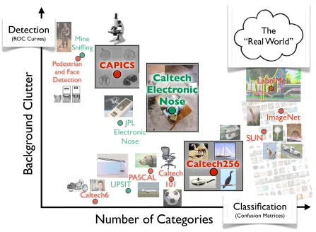
1.1 A rough illustration of machine vision (red) and olfaction (green) tasks lying in and between the regimes of classification and detection. While early problems in vision tended to cluster along either axis, more recent datasets have driven progress further towards the top right. The three projects discussed in this paper are the Caltech-256, the Caltech Electronic Nose and the Caltech Automated Pollen Identification and Counting System (CAPICS). Each is an attempt to take small steps towards the ultimate goal of a system that can robustly detect and classify thousands of categories in the “real world” (upper right). . . 2

2.1 Examples of a 1, 2 and 3 rating for images downloaded using the keyword dice. . . . 6

2.2 Summary of Caltech image datasets. There are actually 102 and 257 categories if the

clutter categories in each set are included. . . . 7

(14)

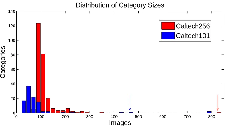
2.4 Histogram showing number of images per category. Caltech-101’s largest categories

faces-easy (435), motorbikes (798), airplanes (800) are shared with Caltech-256. An

additional large category t-shirt (358) has been added. The clutter categories for Caltech-101 (467) and 256 (827) are identified with arrows. This figure should be viewed in color. . . 9

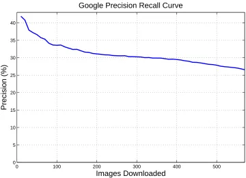
2.5 Precision of images returned by Google. This is defined as the total number of images rated good divided by the total number of images downloaded (averaged over many categories). As more images are download, it becomes progressively more difficult to gather large numbers of images per object category. For example, to gather 40 good images per category it is necessary to collect 120 images and discard 2/3 of them. To gather 160 good images, expect to collect about 640 images and discard 3/4 of them. 10

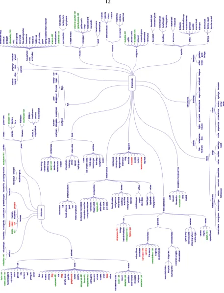
2.6 A taxonomy of Caltech-256 categories created by hand. At the top level these are divided into animate and inanimate objects. Green categories contain images that were borrowed from Caltech-101. A category is colored red if it overlaps with some other category (such as dog and greyhound). . . . 12

2.7 Examples of clutter generated by cropping the photographs of Stephen Shore [103, 104]. . . 13

2.8 Performance of all 256 object categories using a typical pyramid match kernel [67] in a multi-class setting withNtrain= 30. This performance corresponds to the diagonal

(15)

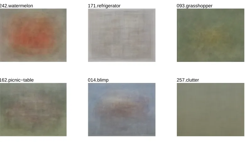
2.9 The mean of all images in five randomly chosen categories, as compared to the mean

clutter image. Four categories show some degree of concentration towards the center

while refrigerator and clutter do not. . . . 17

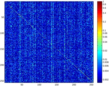
2.10 The256×256matrixMfor the correlation classifier described in subsection 2.4.2. This is the mean of 10 separate confusion matrices generated forNtrain= 30. A log

scale is used to make it easier to see off-diagonal elements. For clarity we isolate the diagonal and row 82 galaxy and describe their meaning in Fig. 2.11. . . . 20

2.11 A more detailed look at the confusion matrix_Mfrom figure 2.10. Top: row 82 shows which categories were most likely to be confused with galaxy. These are: galaxy,

saturn, fireworks, comet and mars (in order of greatest to least confusion). Bottom:

the largest diagonal elements represent the categories that are easiest to classify with the correlation algorithm. These are: self-propelled-lawn-mower, motorbikes-101,

trilobite-101, guitar-pick and saturn. All of these categories tend to have objects that

are located consistently between images. . . 21

2.12 Performance as a function of Ntrain for Caltech-101 and Caltech-256 using the 3

(16)

2.13 Selected rows and columns of the256×256confusion matrixMfor spatial pyramid matching [67] andNtrain= 30. Matrix elements containing 0.0 have been left blank.

The first 6 categories are chosen because they are likely to be confounded with the last 6 categories. The main diagonal shows the performance for just these 12 cate-gories. The diagonals of the other 2 quadrants show whether the algorithm can detect categories which are similar but not exact. . . 24

2.14 ROC curve for three different interest classifiers described in section 2.4.5. These classifiers are designed to focus the attention of the multi-category detectors bench-marked in Figure 2.12. Because Detector B is roughly 200 times faster than A or

C, it represents the best tradeoff between performance and speed. This detector can

accurately detect 38.2% of the interesting (non-clutter) images with a 0.1% rate of false detections. In other words, 1 in 1000 of the images classified as interesting will instead contain clutter (solid red line). If a 1 in 100 rate of false detections is acceptable, the accuracy increases to 58.6% (dashed red line). . . 27

2.15 In general the 256 images are more difficult to classify than the Caltech-101 images. Here we plot performance of the two datasets over a random mix of

Ncategoriesfrom each dataset. Even when the number of categories remains the same,

the Caltech-256 performance is lower. For example atNcategories = 100the

(17)

3.1 A typical one-vs-all multi-class classifier (top) exhaustively tests each image against every possible visual category requiringNcatdecisions per image. This method does

not scale well to hundreds or thousands of categories. Our hierarchical approach uses the training data to construct a taxonomy of categories which corresponds to a tree of classifiers (bottom). In principle each image can now be classified with as few as

log₂Ncat decisions. The above example illustrates this for an unlabeled test image

andNcat = 8. The tree we actually employ has slightly more flexibility as shown in

Fig. 3.4 . . . 33

3.2 Performance comparison between Caltech-101 and Caltech-256 datasets using the spatial pyramid matching algorithm of Lazebnik et al. [67]. The performance of our implementation is almost identical to that reported by the original authors; any per-formance difference may be attributed to a denser grid used to sample SIFT features. This illustrates a standard non-hierarchical approach where authors mainly present the number of training examples and the classification performance, without also plotting classification speed. . . 35

3.3 In general the 256 [55] images are more difficult to classify than the Caltech-101 images. Here we fixNtrain= 30and plot performance of the two datasets over a

random mix ofNcatcategories chosen from each dataset. The solid region represents

a range of performance values for 10 randomized subsets. Even when the number of categories remains the same, the Caltech-256 performance is lower. For example at

(18)

3.4 A simple hierarchical cascade of classifiers (limited to two levels and four categories for simplicity of illustration). We call A, B, C and D four sets of categories as illus-trated in Fig 3.5. Each white square represents a binary branch classifier. Test images are fed into the top node of the tree where a classifier assigns them to either the set A

∪B or the set C∪D (white square at the center-top). Depending on the classification, the image is further classified into either A or B, or C or D. Test images ultimately terminate in one of the 7 red octagonal nodes where a conventional multi-class node

classifier makes the final decision. For a two-level ℓ = 2tree, images terminate in one of the 4 lower octagonal nodes. If ℓ = 0 then all images terminate in the top octagonal node, which is equivalent to conventional non-hierarchical classification. The tree is not necessarily perfectly balanced: A, B, C and D may have different cardinality. Each branch or node classifier is trained exclusively on images extracted from the sets that the classifier is discriminating. See Sec. 3.4 for details. . . 38

3.5 Top-down grouping as described in Sec. 3.3. Our underlying assumption is that cate-gories that are easily confused should be grouped together in order to build the branch classifiers in Fig 3.4. First we estimate a confusion matrix using the training set and a leave-one-out procedure. Shown here is the confusion matrix forNtrain = 10, with

(19)

3.6 Taxonomy discovered automatically by the computer, using only a limited subset of Caltech-256 training images and their labels. Aside from these labels there is no other human supervision; branch membership is not hand-tuned in any way. The taxonomy is created by first generating a confusion matrix forNtrain= 10and

recur-sively dividing it by spectral clustering. Branches and their categories are determined solely on the basis of the confusion between categories, which in turn is based on the feature-matching procedure of spatial pyramid matching. To compare this with some recognizably human categories we color code all the insects (red), birds (yellow), land mammals (green) and aquatic mammals (blue). Notice that the computer’s hier-archy usually begins with a split that puts all the plant and animal categories together in one branch. This split is found automatically with such consistency that in a third of all randomized training sets not a single category of living thing ends up on the opposite branch. . . 41

(20)

3.8 Comparison of three different methods for generating taxonomies. For each taxon-omy we vary the number of branch comparisons prior to final classification, as illus-trated in Fig. 3.4. This results in a tradeoff between performance and speed as one moves between two extremes A and C. Randomly generated hierarchies result in poor cascade performance. Of the three methods, taxonomies based on Spectral Cluster-ing yield marginally better performance. All three curves measure performance vs. speed forNcat= 256andNtrain= 10. . . 44

3.9 Cascade performance / speed trade-off as a function ofNtrain. Values ofNtrain= 10

andNtrain= 50result in a 5-fold and 20-fold speed increase (respectively) for a fixed

10% performance drop. . . 45

4.1 Dr. James House stands next to a modern-day Burkard pollen sampler located on the roof of Keck Laboratory at Caltech (left). The basic techniques used to collect pollen date back to the work of J. M. Hirst in the early 1950’s (right). . . 48

(21)

4.3 Pollen is classified using a cascade of progressively more expensive classification stages. The size of each yellow diamond represents the complexity of the classifier stage, with successive stages passing fewer and fewer candidates to the slower, more refined classifiers downstream. . . 52

4.4 In a Mechanical Turk experiment, test subjects are asked to classify the pollen on the right side using a randomized set of training examples provided on the left. . . 54

4.5 Test subjects do not see the expert classification (red) or the computer classification (green). While the computer “misclassified” this particular birch sample as oak, the true ground-truth classification could actually be either, as demonstrated by visually similar instances circled in each class. . . 55

4.6 Mechanical Turk test subjects and the automated system make similar classification mistakes. Overall performance is 60.3% averaged over all test subjects, 70.9% av-eraged over the 8 most reliable test subjects, and 80.2% for the automated count. Confusion matrices may vary significantly among individual test subjects, as shown by 9 individual confusion matrices for the 9 test subjects with the largest number of classifications. . . 56

(22)

4.8 Daily automated pollen counts for 2012. The total count is broken down into color bands showing the contribution from individual species. Integrated counts for the year are displayed in the legend. The system can count a month’s worth of pollen in 1 day when scanning the slide as an expert would, utilizing less than .1% of the total collecting area. It is thus nearly fast enough to scan the entire slide which would drastically reduce the sampling error and bias. We continue to optimize the code towards this eventual goal. . . 59

(23)

6.2 (a) A sniff consisted of 7 individual subsniffss1...s7of sensor data taken as the valve

switched between a single odorant and reference air. From this data a7×4= 28 size featuremwas generated representing the measured power in each of the 7 subsniffs

iover 4 fundamental harmonicsj. For comparison purposes a simple amplitude fea-ture differenced the top and bottom 5% quartiles of ∆_RR in each subsniff. (b) As the switching frequencyf increased by powers of 2 so did the number of pulses, so that the time period T was constant for all but the first subsniff. (c) To illustrate howm

was measured we show the harmonic decomposition of just s4, highlighted in (a).

The corresponding measurements m4j were the integrated spectral power for each of 4 harmonics. Higher-order harmonics suffered from attenuation due to the lim-ited time-constant of the sensors but had the advantage of being less susceptible to slow signal drift. Fitting a1/fn_{noise spectrum to the average indoor and outdoor} fre-quency response of our sensors in the absence of any odorants illustrates why higher-frequency switching and higher-order harmonics may be especially advantageous in outdoors environments. . . 70

(24)

7.1 Classification performance for the University of Pittsburgh Smell Identification Test (UPSIT) and the Common Household Odors Dataset (CHOD) for different sniff sub-sets using 4 and 16 categories for training and testing. For control purposes data were also acquired with empty odorant chambers. Compared with using the entire sniff (top), the high-frequency subsniffs (2nd row) outperformed the low-frequency subsniffs (bottom) especially for Ncat = 16. The dotted lines show the expected

performance for random guessing. . . 75

7.2 Classification error for all three datasets taken indoors and outdoors while varying the number of sensors and the number of categories used for training and testing. Each dotted colored line represents the mean performance over randomized subsets of 2, 4, 6 and 8 sensors out of the available 10. To illustrate this behavior for a single value of Ncat, gray vertical lines were used to mark the error averaged over randomized

sets of 16 odor categories for the indoor and outdoor datasets. When the number of sensors increased from 4 to 10, the indoor error (left line) decreased by < 2% for the CHOD and UPSIT while the outdoor error (right line) decreased by 4-7%. The Control error is also important because deviations from random chance when no odor categories are present may suggest sensitivity to environmental factors such as water vapor. The indoor error for both 4 and 10 sensors remained consistent with 93.75% random chance while the outdoor error increased from 85.9% to 91.7% . . . 77

(25)

(26)

(27)

Chapter 1

Introduction

My first project in the Caltech Vision Lab was to collect the Caltech-256 Image Dataset[55] with the help of paid workers and other lab members. It was collected using the same methods used to create the Caltech-101[69] years earlier. Starting with images downloaded from the Google and Picsearch search engines with a query such as “airplane”, annotators removed those images that did not fit the visual category. This followup to the Caltech-101 not only increased the number of available cate-gories to 256 but also increased the total image count from∼9000 to 30000. Individual categories were better represented1 with larger variation in pose and background environment. An additional

clutter category based on the photographs of Stephen Shore [103, 104] was added to represent the

appearance of images possessing no distinct visual category. The Caltech-256 was successful in the sense that it challenged the computer vision community to scale image classification algorithms to a larger number and variety of categories than were previously available2. One the other hand, the classification of static images is in many ways a synthetic task which does not address the very real problem of actually finding instances of visual categories in the world we observe. Despite attempts to include images with varying degrees of clutter one is still merely classifying photographs with all the inherent biases that photography implies.

Face detection[112, 44] and pedestrian detection[27] algorithms tackle a different class of the 1_{at least 80 images per categories instead of 31}

(28)

[image:28.612.46.493.69.397.2]

Figure 1.1: A rough illustration of machine vision (red) and olfaction (green) tasks lying in and between the regimes of classification and detection. While early problems in vision tended to cluster along either axis, more recent datasets have driven progress further towards the top right. The three projects discussed in this paper are the Caltech-256, the Caltech Electronic Nose and the Caltech Automated Pollen Identification and Counting System (CAPICS). Each is an attempt to take small steps towards the ultimate goal of a system that can robustly detect and classify thousands of categories in the “real world” (upper right).

computer vision problem: visual object detection. Applications typically focus on finding one or several specific visual categories “in the wild” without attempting to classify the full range of observable objects. By comparison, humans are able to distinguish more than 5000 visual categories[10] in complex environments using a variety of different recognition systems all working in tandem[74].

(29)

of categories that can be classified. The y-axis represents the detection difficulty as the degree of background clutter, that is, how much “haystack” there is for each “needle” that the automated system is trying to detect.

Since the release of the Caltech-256 in 2007, image datasets with over a thousand categories have emerged such as SUN[17], LabelMe[109] and Imagenet[21]. At least some subset of each of these datasets is annotated so that the visual objects are not only labelled but localized. These and other datasets are helping to push machine vision algorithms closer to the ideal of a system that could accurately detect and classify thousands of object categories in a variety of visual environments[65, 64, 71, 92, 18, 72]. Though it is a much younger field, machine olfaction is also beginning to confront some of these same challenges.

This thesis is a collection of 4 papers3which each represent small steps towards the top-right of Fig. 1.1. Chapter 2 discusses the collection methodology for the Caltech-256 and the challenges it presents. This includes spatial pyramid matching [67] classification performance, as well as exper-iments using the new clutter category to create a fast foreground/background “objectness” detector to be used in conjunction with multi-class classifiers. Chapter 3 presents a novel method for cre-ating detailed taxonomies of visual categories using a classifier’s inter-category confusion. To take advantage of such taxonomies we experiment with a simple learning framework that combines an initial decision-tree stage with a final multi-class classification stage to obtain some of the advan-tages of each. The resulting 5 to 20-fold increase in classification speed suggests that taxonomies may be employed in a divide-and-conquer classification strategy to scale existing computer vision algorithms to larger numbers of categories than might otherwise be computationally feasible.

Chapter 4 describes The Caltech Automated Pollen Identification and Counting System (CAPICS). While the pollen classification task involves fewer object categories than the Caltech-256, the

(30)

tor burden is much higher since the microscope slides contain 1,000 to 10,000 unwanted particles for each particle of pollen. To achieve acceptable speed and performance our system uses a seg-mentation stage coupled to a cascade of detectors followed by a final multi-class classification stage. Initial results and potential applications are discussed.

(31)

Chapter 2

The Caltech-256

We introduce a challenging set of 256 object categories containing a total of 30607 images. The original Caltech-101 [69] was collected by choosing a set of object categories, downloading exam-ples from Google Images and then manually screening out all images that did not fit the category. Caltech-256 is collected in a similar manner with several improvement: a) the number of categories is more than doubled, b) the minimum number of images in any category is increased from 31 to 80, c) artifacts due to image rotation are avoided and d) a new and larger clutter category is introduced for testing background rejection. We suggest several testing paradigms to measure classification performance, then benchmark the dataset using two simple metrics as well as a state-of-the-art spa-tial pyramid matching [67] algorithm. Finally we use the clutter category to train an interest detector which rejects uninformative background regions.

2.1 Introduction

(32)

1. good

2. bad

3. not applicable

Figure 2.1: Examples of a 1, 2 and 3 rating for images downloaded using the keyword dice.

performance. The Coil set contains objects placed on a black background with no clutter. The 6. consists of 3738 images of cars, motorcycles, airplanes, faces and leaves. The Caltech-101 is similar in spirit to the Caltech-6 but has many more object categories, as well as hand-clicked silhouettes of each object. The MIT-CSAIL database contains more than 77,000 objects labeled within 23,000 images that are shown in a variety of environments. The number of labeled objects, object categories and region categories increases over time thanks to a publicly available LabelMe [98] annotation tool. The PASCAL VOC 2006 database contains 5,304 images where 10 categories are fully annotated. Finally, the Graz set contains three object categories in difficult viewing conditions. These and other standardized sets of categories allow users to compare the performance of their algorithms in a consistent manner.

Here we introduce the Caltech-256. Each category has a minimum of80images (compared to the Caltech-101 where some classes have as few as31 images). In addition we do not left-right align the object categories as was done with the Caltech-101, resulting in a more formidable set of categories.

(33)

The categories were hand-picked by the authors to represent a wide variety of natural and artificial objects in various settings. The organization is simple and the images are ready to use, without the need for cropping or other processing. In most cases the object of interest is prominent with a small or medium degree of background clutter.

Dataset Released Categories Images Images Per Category

Total Min Med Mean Max

Caltech-101 2003 102 9144 31 59 90 800

Caltech-256 2006 257 30607 80 100 119 827

Figure 2.2: Summary of Caltech image datasets. There are actually 102 and 257 categories if the

clutter categories in each set are included.

In Section 2.2 we describe the collection procedures for the dataset. In Section 2.3 we give paradigms for testing recognition algorithms, including the use of the background clutter class. Example experiments are provided in Section 2.4. Finally in Section 2.5 we conclude with a general discussion of advantages and disadvantages of the set.

2.2 Collection Procedure

The object categories were assembled in a similar manner to the Caltech-101. A small group of vision dataset users were asked to supply the names of roughly 300 object categories. Images from each category were downloaded from both Google and PicSearch using scripts . We required that the minimum size in either aspect be 100 with no upper range. Typically this procedure resulted in about400₋600images from each category. Duplicates were removed by detecting images which contained over15similar SIFT descriptors [76].

The images obtained were of varying quality. We asked 4 different subjects to rate these images using the following criteria:

(34)

0 200 400 600 800 1000 1200 0

500 1000 1500

640x480

800x600

1024x768

sqrt(width*height)

Images

Image Size and Aspect Ratio

0 0.5 1 1.5 2 2.5 3 3.5 4

0 1000 2000 3000 4000 5000

width/height

Images

2/3 3/4 1

4/3

[image:34.612.84.469.81.354.2]

3/2

Figure 2.3: Distribution of image sizes as measured by√width_·height, and aspect ratios as mea-sured bywidth/height. Some common image sizes and aspect ratios that are overrepresented are labeled above the histograms. Overall in Caltech-256 the mean image size is 351 pixels while the mean aspect ratio is 1.17.

2. Bad: A confusing, occluded, cluttered or artistic example 3. Not Applicable: Not an example of the object category

Sorters were instructed to label the image bad if either: (1) the image was very cluttered, (2) the image was a line drawing, (3) the image was an abstract artistic representation, or (4) the object within the image occupied only a small fraction of the image. If the image contained no examples of the visual category it was labeled not applicable. Examples of each of the 3 ratings are shown in Fig. 2.1.

(35)

0 100 200 300 400 500 600 700 800 0

20 40 60 80 100 120 140

Images

2.3 Benchmarks

Previous datasets suffered from non-standard testing and training paradigms, making direct com-parisons of certain algorithms difficult. For instance, results reported by Grauman [52] and Berg [9] were not directly comparable as Berg used only 15 training while Grauman used 30 training ex-amples3. Some authors used the same number of test examples for each category, while other did not. This can be confusing if the results are not normalized in a consistent way. For consistent comparisons between different classification algorithms, it is useful to adopt standardized training and testing procedures

(41)

0 10 20 30 40 50 60 70 80 90 100

car−side−101: 252 _{faces−easy−101: 253} airplanes−101: 251 _{motorbikes−101: 145} leopards−101: 129 _{self−propelled−lawn−mower: 182} tower−pisa: 225 _{trilobite−101: 230} watch−101: 240 _{desk−globe: 053}

ketch−101: 123 _{hibiscus: 103} sunflower−101: 204 _{brain−101: 020} zebra: 250 _{mars: 137} saturn: 177 _{galaxy: 082} bonsai−101: 015 _{guitar−pick: 094} sheet−music: 184 _{menorah−101: 140} revolver−101: 172 _{fireworks: 073} teepee: 214 _{fire−truck: 072} license−plate: 130 _{rainbow: 170} homer−simpson: 104 _{grand−piano−101: 091} photocopier: 161 _{tennis−court: 217} cartman: 032 _{lightning: 133} buddha−101: 022 _{hawksbill−101: 100} ewer−101: 066 _{chandelier−101: 036} golden−gate−bridge: 086 _{vcr: 237} harp: 098 _{hourglass: 110} backpack: 003 _{french−horn: 077} touring−bike: 224 _{yarmulke: 248} coffee−mug: 041 _{grapes: 092} tombstone: 222 _{comet: 044} video−projector: 238 _{hamburger: 095} laptop−101: 127 _{washing−machine: 239} waterfall: 241 _{boom−box: 016} breadmaker: 021 _{telephone−box: 215} eyeglasses: 067 _{cereal−box: 035} diamond−ring: 054 _{stained−glass: 200} binoculars: 012 _{computer−monitor: 046} pci−card: 157 _{treadmill: 227} tennis−shoes: 255 _{helicopter−101: 102} chess−board: 037 _{palm−tree: 154} hot−tub: 109 _{microwave: 142} paper−shredder: 156 _{school−bus: 178} rotary−phone: 174 _{human−skeleton: 112} lightbulb: 131 _{umbrella−101: 235} eiffel−tower: 062 _{frying−pan: 081} mountain−bike: 146 _{elephant−101: 064} porcupine: 164 _{top−hat: 223} cd: 033 _{skyscraper: 187} beer−mug: 010 _{harpsichord: 099} tomato: 221 _{tripod: 231} t−shirt: 232 _{american−flag: 002} baseball−glove: 005 _{starfish−101: 201} theodolite: 219 _{head−phones: 101} roulette−wheel: 175 _{frisbee: 079} hot−air−balloon: 107 _{covered−wagon: 050} saddle: 176 _{megaphone: 139} football−helmet: 076 _{tweezer: 234} pez−dispenser: 160 _{spaghetti: 196} teapot: 212 _{killer−whale: 124} picnic−table: 162 _{sextant: 183} steering−wheel: 202 _{coin: 043} swiss−army−knife: 208 _{elk: 065} wine−bottle: 246 _{skunk: 186} house−fly: 111 _{teddy−bear: 213} kangaroo−101: 121 _{pyramid: 167} ipod: 117 _{billiards: 011} fire−extinguisher: 070 _{mattress: 138} segway: 181 _{llama−101: 134} ak47: 001 _{toad: 256} snowmobile: 192 _{toaster: 220} triceratops: 228 _{chopsticks: 039} refrigerator: 171 _{scorpion−101: 179} electric−guitar−101: 063 _{iris: 118} fern: 068 _{minaret: 143} palm−pilot: 153 _{bathtub: 008} microscope: 141 _{stirrups: 203} tennis−racket: 218 _{ostrich: 151} gorilla: 090 _{cowboy−hat: 051} calculator: 027 _{doorknob: 058} car−tire: 031 _{jesus−christ: 119} welding−mask: 243 _{bulldozer: 023} gas−pump: 083 _{harmonica: 097} cormorant: 049 _{sneaker: 191} soccer−ball: 193 _{penguin: 158} giraffe: 084 _{mandolin: 136} necktie: 149 _{octopus: 150} tambourine: 211 _{butterfly: 024} light−house: 132 _{raccoon: 168} owl: 152 _{hummingbird: 113} bowling−pin: 018 _{cake: 026} computer−keyboard: 045 _{joy−stick: 120} sushi: 206 _{blimp: 014} tricycle: 229 _{bowling−ball: 017} floppy−disk: 075 _{minotaur: 144} lathe: 128 _{cactus: 025} speed−boat: 197 _{xylophone: 247} radio−telescope: 169 _{wheelbarrow: 244} crab−101: 052 _{computer−mouse: 047} hammock: 096 _{boxing−glove: 019} duck: 060 _{ibis−101: 114} superman: 205 _{swan: 207} baseball−bat: 004 _{tennis−ball: 216} watermelon: 242 _{chimp: 038} ice−cream−cone: 115 _{birdbath: 013} cockroach: 040 _{horseshoe−crab: 106} pram: 165 _{bear: 009} cannon: 029 _{spider: 198} centipede: 034 _{fried−egg: 078} mussels: 148 _{smokestack: 188} windmill: 245 _{basketball−hoop: 006} fighter−jet: 069 _{screwdriver: 180} sword: 209 _{fire−hydrant: 071} playing−card: 163 _{unicorn: 236} dice: 055 _{mushroom: 147} paperclip: 155 _{socks: 194} greyhound: 254 _{dolphin−101: 057} camel: 028 _{tuning−fork: 233} flashlight: 074 _{grasshopper: 093} coffin: 042 _{bat: 007} goat: 085 _{golf−ball: 088} goose: 089 _{frog: 080} traffic−light: 226 _{goldfish: 087} canoe: 030 _{dumb−bell: 061} iguana: 116 _{snail: 189} kayak: 122 _{mailbox: 135} people: 159 _{drinking−straw: 059} horse: 105 _{spoon: 199} conch: 048 _{knife: 125}

snake: 190 _{syringe: 210}

yo−yo: 249 _{dog: 056}

praying−mantis: 166 _{hot−dog: 108}

soda−can: 195 _{ladder: 126}

rifle: 173 _{skateboard: 185}

Performance By Category

Performance (%)

←

Worse Performance Better Performance

→

Figure 2.8: Performance of all 256 object categories using a typical pyramid match kernel [67] in a multi-class setting withNtrain = 30. This performance corresponds to the diagonal entries of

(42)

2.3.1 Performance

First we selectNtrainand Ntest images from each class to train and test the classifier. Specifically

Ntrain=5, 10, 15, 20, 25, 30, 40 andNtest = 25.

Each test image is assigned to a particular class by the classifier. Performance of each classCcan be measured by determining the fraction of test examples for classCwhich are correctly classified as belonging to class _C. The cumulative performance is calculated by counting the total number of correctly classified test imagesNtest within each ofNclass classes. It is of course important to

weight each class equally in this metric. The easiest way to guarantee this is to use the same number of test images for each class. Finally, better statistics are obtained by averaging the above procedure multiple times (ideally at least 10 times) to reduce uncertainty.

The exactly value ofNtest is not important. For Caltech-101 values higher thanNtrain = 30

are impossible since some categories contain only 31 images. However Caltech-256 has at least 80 images in all categories. Even a training set size of Ntrain = 75 leaves Ntest ≥ 5 available for

testing in all categories.

The confusion matrixMij illustrates classification performance. It is a table where each ele-menti, jstores the fraction of the test images from category_Ci that were classified as belonging to

Cj. Note that perfect classification would result in a table with ones along the main diagonal. Even

if such a classification method existed, this ideal performance would not be reached for several rea-sons. Images in most categories contain instances of other categories, which is a built-in source of confusion. Also our sorting procedure is never prefect; there are bound to be some small fraction of incorrectly classified images in a dataset of this size.

Since the last 6 categories are redundant with existing categories, and clutter indicates the ab-sence of any category, one might argue that only categoriesC1...C250are appropriate for generating

(43)

measur-242.watermelon 171.refrigerator 093.grasshopper

[image:43.612.140.530.74.300.2]

162.picnic−table 014.blimp 257.clutter

Figure 2.9: The mean of all images in five randomly chosen categories, as compared to the mean

clutter image. Four categories show some degree of concentration towards the center while refrig-erator and clutter do not.

ing overall performance is that they are among the easiest to identify. Thus removing them makes the detection task more challenging4.

However for better clarity and consistency, we suggest that authors remove only the clutter category, generate a 256x256 confusion matrix with the remaining categories, and report their per-formance results directly from the diagonal of this matrix5. Is also useful for authors to post the confusion matrix itself - not just the mean of the diagonal.

2.3.2 Localization and Segmentation

Both Caltech-101 and the Caltech-256 contain categories in which the object may tend to be cen-tered (Fig. 2.9). Thus, neither set is appropriate for localization experiments, in which the algorithm must not only identify what object is present in the image but also where the object is.

Furthermore we have not manually annotated the images in Caltech-256 so there is presently no 4_{As shown in figure 2.13, categories}_C

251,C252andC253each yield performance above90%

(44)

ground truth for testing segmentation algorithms.

2.3.3 Generality

Why not remove the last 6 categories from the dataset altogether? Closely related categories can provide useful information that is not captured by the standard performance metric. Is a certain

greyhound classifier also good at identifying dog, or does it only detect specific breeds? Does a

sneaker detector also detect images from tennis-shoe, a word which means essentially the same

thing? If it does not, one might worry that the algorithm is over-training on specific features of the dataset which do not generalize to visual categories in the real world.

For this reason we plot rows 251..256 of the confusion matrix along with the categories which are most similar to these, and discuss the results in section 2.3.3.

Consider the example of a Mars rover that moves around in its environment while taking pictures. Raw performance only tells us the accuracy with which objects are identified. Just as important is the ability to identify where there is an object of interest and where there is only uninteresting background. The rover cannot begin to understand its environment if background is constantly misidentified as an object.

The rover example also illustrates how the meaning of the word background is strongly depen-dent on the environment and the application. Our choice of background images for Caltech-256, as described in 2.2.4, is meant to reflect a variety of common (terrestrial) environments.

(45)

search window of varied size scans across an image employing some sort of bird classifier. Each true positive marks a successful detection of a bird inside the scan window while each false positive indicates an erroneous detection.

What do positive and negative mean in the context of multi-class classification? Consider a two-step process in which each search window is evaluated by a cascade [112] of two classifiers. The first classifier is an interest detector that decides whether a given window contains a object category or background. Background regions are discarded to save time, while all other images are passed to the second classifier. This more expensive multi-class classifier now attempts to identify which of the remaining 256 object categories best matches the region as described in 2.3.1.

Our ROC curve measures the performance of several interest classifiers. A false positive is any

clutter image which is misclassified as containing an object of interest. Likewise true positive refers

to an object of interest that is correctly identified. Here “object of interest” means any classification besides clutter.

2.4 Results

In this section we describe two simple classification algorithms as well as the more sophisticated spatial pyramid matching algorithm of Lazebnik, Schmid and Ponce [67]. Performance, generality and background rejection benchmarks are presented as examples for discussion.

2.4.1 Size Classifier

Our first classifier used only the width and height of each image as features. During the training phase, the width and height of all256·Ntrainimages are stored in a 2-dimensional space. Each test

(46)

50 100 150 200 250 50

100

150

200

250 0.002

[image:46.612.101.474.87.383.2]

0.004 0.006 0.008 0.01 0.02 0.04 0.06 0.08 0.1 0.2 0.4 0.6 0.8 1

Figure 2.10: The256_×256 matrix_Mfor the correlation classifier described in subsection 2.4.2. This is the mean of 10 separate confusion matrices generated forNtrain = 30. A log scale is used

to make it easier to see off-diagonal elements. For clarity we isolate the diagonal and row 82 galaxy and describe their meaning in Fig. 2.11.

As shown in Fig. 2.12, this algorithm identifies the correct category for an image3.7_±0.6%of the time whenNtrain= 30.

(47)

0 50 100 150 200 250 0

0.05 0.1 0.15 0.2 0.25 0.3 0.35

Row 82: "galaxy"

082.galaxy

177.saturn

073.fireworks

044.comet _137.mars

0 50 100 150 200 250

0 0.1 0.2 0.3 0.4 0.5 0.6 0.7 0.8

Diagonal

182.self−propelled−lawn−mower 145.motorbikes−101

230.trilobite−101

[image:47.612.96.546.104.574.2]

094.guitar−pick 177.saturn

Figure 2.11: A more detailed look at the confusion matrix M from figure 2.10. Top: row 82 shows which categories were most likely to be confused with galaxy. These are: galaxy, saturn,

fireworks, comet and mars (in order of greatest to least confusion). Bottom: the largest diagonal

(48)

2.4.2 Correlation Classifier

The next classifier we employed was a correlation based classifier. All images were resized to

Ndim×Ndim, desaturated and normalized to have unit variance. The nearest neighbor was computed in theNdim2-dimensional space of pixel intensities. This is equivalent to finding the training image that correlates best with the test image, since

<(X−Y)2 >=< X2 >+< Y2>−2< XY >=−2< XY >

for imagesX,Y with unit variance. Again we use the 1-norm instead of the 2-norm because it is faster to compute and yields better classification performance.

Performance of7.6±0.7%atNtrain = 30 is computed by taking the mean of the diagonal of

the confusion matrix in Fig. 2.10.

2.4.3 Spatial Pyramid Matching

As a final test we re-implement the spatial pyramid matching algorithm of Lazebnik, Schmid and Ponce [67] as faithfully as possible. In this procedure an SVM kernel is generating from matching scores between a set of training images. Their published Caltech-101 performance atNtrain = 30

was64.6±0.8%. Our own performance is practically the same.

As shown in Fig. 2.12, performance on Caltech-256 is roughly half the performance achieved on Caltech-101. For example at Ntrain = 30 our Caltech-256 and Caltech-101 performance are

(49)

0 5 10 15 20 25 30 35 40 0

10 20 30 40 50 60 70

N

train

Performance (%)

Caltech−101 / Caltech−256 Performance

Caltech−101 SPM

SVM−KNN [3] SPM [2]

[image:49.612.107.505.71.395.2]

Caltech−256 SPM Correlation Size

Figure 2.12: Performance as a function ofNtrainfor Caltech-101 and Caltech-256 using the 3

algo-rithms discussed in the text. The spatial pyramid matching algorithm is that of Lazebnik, Schmid and Ponce [67]. We compare our own implementation with their published results, as well as the SVM-KNN approach of Zhang, Berg, Maire and Malik [120].

2.4.4 Generality

Fig. 2.13 shows the confusion between six categories and their six confounding categories. We define the generality as the mean of the off-quadrant diagonals divided by the mean of the main diagonal. In this case, forNtrain= 30, the generality isg= 0.145.

(50)

12.5 0.5 0.5 5.0 0.5 25.0 0.5 0.5 0.5 1.0 0.5 2.0 5.0 2.0 1.0 5.5 0.5 0.5 1.5 3.5 0.5 2.5 0.5 1.0 24.5 22.0 0.5 0.5 8.5 10.5 1.0 94.5 1.0 100.0 0.5 98.5 0.5 0.5 1.0 2.0 0.5 10.5 1.0 1.0 15.0 0.5 50.0 1.5 0.5 3.5 30.5

069 031 159 056 191 080 251 252 253 254 255 256 069.fighter−jet 031.car−tire 159.people 056.dog 191.sneaker 080.frog 251.airplanes−101 252.car−side−101 253.faces−easy−101 254.greyhound 255.tennis−shoes 256.toad

[image:50.612.81.462.81.355.2]

0 % 10 % 20 % 30 % 40 % 50 % 60 % 70 % 80 % 90 % 100 %

Figure 2.13: Selected rows and columns of the256_×256confusion matrix_Mfor spatial pyramid matching [67] andNtrain = 30. Matrix elements containing 0.0 have been left blank. The first 6

categories are chosen because they are likely to be confounded with the last 6 categories. The main diagonal shows the performance for just these 12 categories. The diagonals of the other 2 quadrants show whether the algorithm can detect categories which are similar but not exact.

six categories were completely indistinguishable. Such a classifier is not discriminating enough to differentiate between airplanes and the more specific category fighter-jet, or between people and their faces. In other words, the classifier generalizes so well about similar object classes that it may be considered too sloppy for some applications.

In practice the desired value of g depends on the needs of the customer. Lower values of g

(51)

As shown in Figure 2.13, a spatial pyramid matching classifier does indeed confuse tennis-shoes and sneakers the most. This is a reassuring sanity check. To a lesser extent the object categories

frog/toad, dog/greyhound, fighter-jet/airplanes and people/faces-easy are also confused.

Confusion between car-tire and car-side is entirely absent. This seems surprising since tires are such a conspicuous feature of cars when viewed from the side. However the tires pictured in

car-tire tend to be much larger in scale than those found in car-side. One reasonable hypothesis is

that the classifier has limited scale-invariance: objects or pieces of objects are no longer recognized if their size changes by an order of magnitude. This characteristic of the classifier may or may not be important, depending on the application. Another hypothesis is that the classifier relies not just on the presence of individual parts, but on their relationship to one another.

In short, generality defines a trade-off between classifier precision and robustness. Our metric for generatinggis admittedly crude because it uses only six pairs of similar categories. Nonetheless generating a confusion matrix like the one shown in Figure 2.13 can provide a useful sanity check, while exposing features of a particular classifier that are not apparent from the raw performance benchmark.

Returning to the example of a Mars rover, suppose that the rover’s camera is used to scan across the surface of the planet. Because there may be only one interesting object in103_-₁₀5 _{images, the}

interest detector must have a low rate of false detections in order to be effective. As illustrated in figure 2.14 this is a challenging problem, particularly when the detector must accommodate hundreds of different object categories that are all considered interesting.

(52)

before the classifier is an SVM with a spatial pyramid matching kernel [67]. The margin threshold is adjusted in order to trace out a full ROC curve6.

Interest Ntrain Speed Description

Detector _C1...C256 C257 (images/sec)

A 30 512 24 Modified 257-category classifier

B 2 512 4600 Fast two-category classifier

C 30 30 25 Ordinary 257-category classifier

First let us consider Interest Detector C. This is the same detector that was employed for rec-ognizing object categories in section 2.4.3. The only differences is that 257 categories are used instead of 256. Performance is poor because only 30 clutter images are used during training. In other words, clutter is treated exactly like any other category.

Interest Detector A corrects the above problem by using 512 training images from the clutter

category. Performance improves because their is now a balance between the number of positive and negative examples. However the detector is still slow because it is a attempts to recognize 257 different object categories in every single image or camera region. This is wasteful if we expect the vast majority of regions to contain irrelevant clutter which is not worth classifying. In fact this detector only classifies about 25 images per second on a 3 GHz Pentium-based PC.

Interest Detector B trains on 512 clutter images and 512 images taken from the other 256 object

categories. These two groups of images are assigned to the categories uninteresting and interesting, respectively. This B classifier is extremely fast because it combines all the interesting images into a single category instead of treating them as 256 separate categories. On a typical 3GHz Pentium processor this classifier can evaluate 4600 images (or scan regions) per second.

It may seem counter-intuitive to group two images from each category C1...C256 into a huge

(53)

0.1 1.0 10 100 0

10 20 30 40 50 60 70 80 90 100

False Positives (%)

True Positives (%)

ROC

Interest Detector A Interest Detector B Interest Detector C

Figure 2.14: ROC curve for three different interest classifiers described in section 2.4.5. These classifiers are designed to focus the attention of the multi-category detectors benchmarked in Fig-ure 2.12. Because Detector B is roughly 200 times faster than A or C, it represents the best tradeoff between performance and speed. This detector can accurately detect 38.2% of the interesting (non-clutter) images with a 0.1% rate of false detections. In other words, 1 in 1000 of the images classi-fied as interesting will instead contain clutter (solid red line). If a 1 in 100 rate of false detections is acceptable, the accuracy increases to 58.6% (dashed red line).

meta-category, as is done with Interest Detector B. What exactly is the classifier training on? What makes an image interesting? What if we have merely created a classifier that detects the photo-graphic style of Stephen Shore? For these reasons any classifier which implements attention should be verified on a variety of background images, not just those inC257. For example the Caltech-6

(54)

4 6 8 10 20 40 60 80 100 200 10

20 30 40 50 60 70 80 90 100

Performance as a Function of the Number of Categories

Performance (%)

N

Caltech−101

Caltech−256

Figure 2.15: In general the Caltech-256 images are more difficult to classify than the Caltech-101 images. Here we plot performance of the two datasets over a random mix ofNcategories from each

dataset. Even when the number of categories remains the same, the Caltech-256 performance is lower. For example atNcategories = 100the performance is∼60% lower.

2.5 Conclusion

Thanks to rapid advances in the vision community over the last few years, performance over60%on the Caltech-101 has become commonplace. Here we present a new Caltech-256 image dataset, the largest set of object categories available to our knowledge. Our intent is to provide a freely available set of visual categories that does a better job of challenging today’s state-of-the-art classification algorithms.

For example, spatial pyramid matching [67] withNtrain = 30achieves performance of67.6%

(55)

exam-ples. As classification performance continues to improve, however, new benchmarks will be needed to reflect the performance of algorithms under realistic conditions. Beyond raw performance, we argue that a successful algorithm should also be able to

• Generalize beyond a specific set of images or categories

• Identify which images or image regions are worth classifying

In order to evaluate these characteristics we test two new benchmarks in the context of Caltech-256. No doubt there are other equally relevant benchmarks that we have not considered. We invite researchers to devise suitable benchmarks and share them with the community at large.

If you would like to share performance results as well as your confusion matrix, please send them to [email protected]. We will try to keep our comparison of performance as up-to-date as possible. For more details seehttp://www.vision.caltech.edu/Image_

(56)

(57)

Chapter 3

Visual Hierarchies

The computational complexity of current visual categorization algorithms scales linearly at best with the number of categories. The goal of classifying simultaneously Ncat = 104 −105 visual

categories requires sub-linear classification costs. We explore algorithms for automatically building classification trees which can have, in principle, logNcat complexity. We find that a greedy

algo-rithm that recursively splits the set of categories into the two minimally confused subsets achieves 5-20 fold speedups at a small cost in classification performance. Our approach is independent of the specific classification algorithm used. A welcome by-product of our algorithm is a very reasonable taxonomy of the Caltech-256 dataset.

3.1 Introduction

(58)

most approaches. There is one exception: cost is logarithmic in the number of models for Lowe [76]. However Lowe’s algorithm was developed to recognize specific objects rather than categories. Its speed hinges on the observation that local features are highly distinctive, so that one may index image features directly into a database of models which is organized like a tree [8]. In the more general case of visual category recognition, local features are not very distinctive, hence one cannot take advantage of this insight.

Humans can recognize between 104and 105object categories [10] and this is a worthwhile and practical goal for machines as well. It is therefore important to understand how to scale classification costs sub-linearly with respect to the number of categories to be recognized. It is quite intuitive that this is possible: when we see a dog we are not for a moment considering the possibility that it might be classified as either a jet-liner or an ice cream cone. It is reasonable to assume that, once an appropriate hierarchical taxonomy is developed for the categories in our visual world, we may be able to recognize objects by descending the branches of this taxonomy and avoid considering irrelevant possibilities. Thus, tree-like algorithms appear to be a possibility worth considering, although formulations need to be found that are more ‘holistic’ than Beis and Lowe’s feature-based indexing [8].

(59)

Class 1 vs others

Class 2 vs others

Decision:

Class 6

1,3,6,8

vs

2,4,5,7

1,6 vs 3,8

2,7 vs 4,5

1 vs 6

3 vs 8

2 vs 7

4 vs 5

Class 3 vs others

Class 4 vs others

Class 5 vs others

Class 6 vs others

Class 7 vs others

Class 8 vs others

Decision:

Class 6

Figure 3.1: A typical one-vs-all multi-class classifier (top) exhaustively tests each image against every possible visual category requiringNcatdecisions per image. This method does not scale well

to hundreds or thousands of categories. Our hierarchical approach uses the training data to construct a taxonomy of categories which corresponds to a tree of classifiers (bottom). In principle each image can now be classified with as few aslog₂Ncatdecisions. The above example illustrates this for an

unlabeled test image andNcat = 8. The tree we actually employ has slightly more flexibility as

shown in Fig. 3.4

3.2 Experimental Setup

The goal of our experiment is to compare classification performance and computational costs when a given classification algorithm is used in the conventional one-vs-many configuration vs our pro-posed hierarchical cascade (see Fig. 3.1).

3.2.1 Training and Testing Data

(60)

performance and ease of implementation. We summarize our implementation in Sec.3.2.2. Our implementation performs as reported by the original authors on Caltech-101. As expected, typical performance on Caltech-256 [55] is lower than on Caltech-101 [69] (see Fig. 3.2). This is due to two factors: the larger number of categories and the more challenging nature of the pictures them-selves. For example some of the Caltech-101 pictures are left-right aligned whereas the Caltech-256 pictures are not. On average a random subset ofNcatcategories from the Caltech-256 is harder to

classify than a random subset of the same number of categories from the Caltech-101 (see Fig. 3.3). Other authors have achieved higher performance on the Caltech-256 than we report here, for example, by using a linear combination of multiple kernels [111]. Our goal here is not to achieve the best possible performance but to illustrate how a typical algorithm can be accelerated using a hierarchical set of classifiers.

The Caltech-256 image set is used for testing and training. We remove the clutter category from Caltech-256 leaving a total ofNcat = 256categories.

3.2.2 Spatial Pyramid Matching

First each image is desaturated, removing all color information. For each of these black-and-white images, SIFT features [76] are extracted along a uniform 72x72 grid using software that is publicly available [84]. An M-word feature vocabulary is formed by fitting a Gaussian mixture model to 10,000 features chosen at random from the training set. This model maps each 128-dimensional SIFT feature vector to a scalar integerm= 1..M whereM = 200is the total number of Gaussians. The choice of clustering algorithm does not seem to affect the results significantly, but the choice of M does. The original authors [67] find that 200 visual words are adequate.

(61)

5 10 15 20 25 30 0

10 20 30 40 50 60 70

N

train

Performance (%)

Caltech−101

Caltech−101(Lazebnik et al.)

Caltech−256

Figure 3.2: Performance comparison between Caltech-101 and Caltech-256 datasets using the spa-tial pyramid matching algorithm of Lazebnik et al. [67]. The performance of our implementation is almost identical to that reported by the original authors; any performance difference may be at-tributed to a denser grid used to sample SIFT features. This illustrates a standard non-hierarchical approach where authors mainly present the number of training examples and the classification per-formance, without also plotting classification speed.

histogram counts the number of times each word 1..M appears in each of the 16 spatial bins. Unlike a bag-of-words approach [53], coarse-grained position information is retained as the features are counted.

(62)

4 6 8 10 20 40 60 80 100 200 10

20 30 40 50 60 70 80 90 100

Performance (%)

N

cat

Caltech−101

Caltech−256

Figure 3.3: In general the 256 [55] images are more difficult to classify than the Caltech-101 images. Here we fixNtrain= 30and plot performance of the two datasets over a random mix of

Ncatcategories chosen from each dataset. The solid region represents a range of performance values

for 10 randomized subsets. Even when the number of categories remains the same, the Caltech-256 performance is lower. For example atNcat = 100the performance is∼ 60% lower (dashed red

line).

training an SVM.

3.2.3 Measuring Performance

Classification performance is measured as a function of the number of training examples. First we select a random but disjoint set ofNtrainandNtesttraining and testing images from each class. All

categories are sampled equally, ie.NtrainandNtestdo not vary from class to class.

Learning and Using Taxonomies for Visual and Olfactory Classification

Classification

Acknowledgements

Abstract

Contents

List of Figures

Chapter 1

Introduction

Chapter 2

The Caltech-256

2.1

Introduction

2.2

Collection Procedure

2.3

Benchmarks

Performance By Category

2.4

Results

Row 82: "galaxy"

Diagonal

Caltech−101 / Caltech−256 Performance

ROC

Performance as a Function of the Number of Categories

Performance (%)

N

categories

Caltech−101

Caltech−256

2.5

Conclusion

Chapter 3

Visual Hierarchies

3.1

Introduction

Class 1 vs others

Class 2 vs others

Decision:

Class 6

1,3,6,8

vs

2,4,5,7

1,6 vs 3,8

2,7 vs 4,5

1 vs 6

3 vs 8

2 vs 7

4 vs 5

Class 3 vs others

Class 4 vs others

Class 5 vs others

Class 6 vs others

Class 7 vs others

Class 8 vs others

Decision:

Class 6

3.2

Experimental Setup

N

train

Performance (%)

Caltech−101

Caltech−101(Lazebnik et al.)

Caltech−256

Performance (%)

N

cat

Caltech−101

Caltech−256