Data Assimilation for Precipitation Nowcasting using Bayesian
Inference
Remi Barillec, Dan Cornford
Neural Computing Research Group, Aston University, Birmingham, B4 7ET, UK
Abstract
This work introduces a new variational Bayes data assimilation method for the stochastic estimation of precipitation dynamics using radar observations for short term probabilistic forecasting (nowcasting). A previously developed spatial rainfall model based on the decomposition of the observed precipitation field using a basis function expansion captures the precipitation intensity from radar images as a set of ‘rain cells’. The prior distributions for the basis function parameters are carefully chosen to have a conjugate structure for the precipitation field model to allow a novel variational Bayes method to be applied to estimate the posterior distributions in closed form, based on solving an optimisation problem, in a spirit similar to 3D VAR analysis, but seeking approximations to the posterior distribution rather than simply the most probable state. A hierarchical Kalman filter is used to estimate the advection field based on the assimilated precipitation fields at two times. The model is applied to tracking precipitation dynamics in a realistic setting, using UK Met Office radar data from both a summer convective event and a winter frontal event. The performance of the model is assessed both traditionally and using probabilistic measures of fit based on ROC curves. The model is shown to provide very good assimilation characteristics, and promising forecast skill. Improvements to the forecasting scheme are discussed.
1. Introduction
Short term forecasts of precipitation fields are of crit-ical importance to hydrologists who rely on them to pre-vent floods [40] or manage sewage systems in real time [56]. Because such applications are usually restricted to specific areas (typically an urbanized zone or the small scale catchment of a river) and deal with events which develop over short periods of time, the forecasting com-munity has to provide hydrologists with precipitation forecasts at high spatial and temporal resolutions, typi-cally referred to as nowcasts. According to [21], precip-itation run-off models could require, in theory, forecasts down to 0.5 km spatial and 1 min temporal resolutions.
Traditional numerical weather prediction (NWP) models replicate the physics of the atmosphere, by solving a system of governing differential equations
Email addresses:[email protected](Remi Barillec), [email protected](Dan Cornford).
together with physics based parameterisations and extrapolating into the future. This requires heavy com-putational power, and considerable computing time. With the advent of ever faster computers, NWP mod-els are starting the be run at resolutions down to 1-4 km[15; 30]. However, two main issues arise when applying NWP models to nowcasting: the existence of a spin up phase during which the incomplete rep-resentation of initial conditions affects the model’s performance, and the fact that at the scales of interest, our understanding of convective processes is still very limited. Recent research projects aimed at increasing that understanding[6] will hopefuly lead to a better formulation of NWP models at small scales.
Because of the reasons mentionned above, it is well acknowledged that NWP models are not particularly suited to the nowcasting problem[20; 21; 33]. There-fore alternative approaches have been developed. Con-strained to run fast and at high resolution, nowcasting systems cannot rely on physics the way NWP
mod-els do. The physical equations driving the process of interest have to be approximated in some way. There are many different ways to model precipitation, rang-ing from image processrang-ing based techniques to purely stochastic approaches. A short review of some models found in the literature is given in Section 2.
An immediate consequence of the approximations applied in nowcasting models is their limited forecast skill. For instance, in advection based nowcasting sys-tems such as the one presented in this work, the as-sumption that the rainfall evolution is dominated by mo-tion is only valid up to a certain time, beyond which the growth and decay of cells become a non negligible source of change. The speed at which forecast skill is lost depends on the nature of the rainfall, with reason-able skill being retained for a few minutes for fast de-veloping convective storms up to a few hours for slowly evolving fronts.
In order to ensure the nowcasting model remains co-herent with the evolution of the true precipitation field, observations of the precipitation field are used to recal-ibrate the model (i.e. adjust its parameters) in real time. The process of incorporating observed information into the model is often called data assimilation.
With the advent of weather radar, frequent measure-ments (one observation every 5 to 15 minutes) with high spatial resolution (1 to 5 km) have become avail-able to the forecasting community [8]. Such advantages quickly made radar data the favourite source of infor-mation for nowcasting models, greatly influencing the range of techniques developed. Although there are other sources of precipitation measurement available (rain-gauges, airborne sensors, satellites), this paper only dis-cusses the problem of radar-based precipitation now-casting, however the framework could easily incorpo-rate other observations in the future.
In the following sections, we introduce a radar-based precipitation model which provides a fully probabilis-tic framework for precipitation nowcasting, with em-phasis on data assimilation . The discussion is organ-ised as follows. Section 2 gives a brief review of recent advances in precipitation nowcasting, while Section 3 outlines the concepts of probabilistic data assimilation. Section 4 then describes the model and its implementa-tion. Results are presented and analysed in Sections 6, 7 and discussed in Section 8.
2. Precipitation nowcasting systems
There have been two main trends in the develop-ment of nowcasting methods. On the one hand,
extrap-olation methods predict the evolution of the observed
rainfall field using object tracking and advection-based techniques, while on the other hand, storm generating methods focus on the birth, growth and dissipation of storms. The latter category can be divided further into
point process models and multifractal models. Both
ex-trapolation and storm generating methods involve, in one way or another, the following components: a spa-tial representation of the precipitation field, a spaspa-tial- spatial-temporal model for its evolution and a means to incor-porate observation data into the model. We present an outline review of such existing methods. The reader is referred to [59; 7; 45] for more extensive reviews.
2.1. Extrapolation methods
Radar-based extrapolation methods rely on the as-sumption that, at the time scales considered, the evolu-tion of the precipitaevolu-tion field is governed by moevolu-tion pri-marily. The UK NIMROD nowcasting system [20; 21] identifies clusters of rainy pixels on radar scans and propagates them forward in time using advection es-timates obtained either by cross-correlation techniques (at short lead times) or NWP wind field forecasts (at longer lead times), with a smoother merging function used to switch between these. Other systems such as the American TITAN [14] and the model of [38] also rely on object tracking methods. The precipitation field is decomposed into a set of elliptic storms, which are then matched from one image to the following. The op-timal trajectory of each storm is determined by min-imising the total mismatch error. Both systems provide support for the merging and splitting of storms. TI-TAN also estimates the growth and decay of storms using linear trends. Another correlation-based method, the TREC/COTREC systems [47; 32], partitions radar scans into smaller regions and matches these regions across subsequent scans using a maximum correlation criterion. Motion vectors are then estimated from the regions’ displacement.
The NCAR Auto-Nowcast system[41] is a complex nowcasting system incorporating a variety of datasets including: radar, lightning and satellite data, wind pro-files and NWP model outputs. The Auto-Nowcast sys-tem makes use of several algorithms to process these datasets into “predictor fields” (e.g. fields of reflectiv-ity, storm growth/decay, accumulated precipitation. . . ). Amongst the algorithms involved, the TREC method is applied to wind field retrieval from radar data and the TITAN algorithm is used to detect storms and es-timate trends in their evolution. A boundary detection
algorithm, coupled with a cloud detection system, al-lows for convergence lines, where storms are expected to occur, to be identified. A physically-based model us-ing fuzzy logic algorithms merges the various predictor fields into a dimensionless likelihood field which is then post-processed to obtain a final prediction estimate.
Bringing further the concept of identifying physical components of the precipitation field, the GANDOLF [46; 21] model considers individual precipitation cells with a conceptual life cycle. The precipitation objects grow and decay according to the life cycle model of [26], while being advected by wind fields estimated from an NWP model. NIMROD, TITAN, GANDOLF and other operational nowcasting systems are discussed more in detail in the context of the Sydney 2000 fore-casting project in [45].
2.2. Point process models
Point process models put the emphasis on estimat-ing the internal dynamics of precipitation fields usestimat-ing statistical representations based on point process mod-els. The models of [48; 11; 50] follow the formalism of [31] in which the occurrence (in space and/or time) of precipitating objects (cells or storms) is governed by Poisson point processes. Storms are defined as areas of constant random precipitation, life-time[48] and veloc-ity [11; 50]. The contributions of overlapping cells are added in both space and time. Estimation of the model’s parameters is achieved by fitting to existing records of precipitation using a method of moments.
Two types of Poisson process for the generation of cells can be found in the literature: the Neyman-Scott process and the Bartlett-Lewis process. In the Neyman-Scott process, storms origins are generated from a Pois-son process. Each storm is given a random number of corresponding precipitation cells, with their origin (in time) distant from the storm’s by a delay drawn from an exponential distribution. Examples using the Neyman-Scott process and derived approaches include [10; 16; 43]. In the Bartlett-Lewis process, storms also originate from a Poisson process in pspace, but a sec-ond Poisson process dictates, for each storm, the time at which cells are initiated. This cell-generating pro-cess is terminated after a sample duration drawn from an exponential distribution. [44; 29; 51] are few of the many applications of the Bartlett-Lewis process to rain-fall modelling. A comparative review of some of these models can be found in [57].
We note here that these models are usually not de-veloped with forecasting or nowcasting in mind rather
being developed providing a valid statistical description of precipitation fields, which might be used for uncondi-tional simulation purposes. In this work we are more in-terested in conditioning the modelled precipitation field on observations, that is data assimilation.
2.3. Multifractal models
In the 1980s, empirical studies have shown that rain-fall fields exhibit statistical invariance with respect to the scale at which they are observed [34; 25] and, as such, could be modelled using random cascade models. In such models, the field at a given scale (i.e. spatial or temporal resolution) can be decomposed into a field at lower scale (higher resolution) by splitting unit re-gions into equal subrere-gions. The intensity of the field at these subregions is determined through a random scal-ing which conserves the overall statistical characteris-tics of the field. Various options for the distribution of the scaling generators are given in [52].
The cascade methodology is naturally expressed us-ing multifractal theory[52; 35] and presents several ad-vantages over object tracking methods: it models the rainfall field at different scales, allows seamless incor-poration of data at various resolutions (fine for radar, coarser for NWP estimates) and in the universal multi-fractal framework described in [52], only require a very small number of parameters to characterise their statis-tics. Dynamics in these models can be modelled by in-cluding time (along with space) in the cascade [13; 4] or using advection based propagation as systems like S-PROG[49] and STEPS[5].
However, a study by [55] underlines the limitations of multifractal models and shows, using several datasets, that assuming the scaling factors to be independent of the scale leads to unrealistic simulation results. The au-thors conclude that “rainfall does not behave like a mul-tifractal process” and that mulmul-tifractal models in which the scaling generators are identically distributed are “in-adequate”, and suggest directions for a new generation of multifractal models. We note that the data assimi-lation method we develop and apply in this paper is equally applicable to cascade like models, where the precipitation field and advection could be computed at each level in the cascade using our variational Bayesian methods.
2.4. Other methods
Other techniques have been applied to the prob-lem of precipitation forecasting. [60] apply to
pre-cipitation nowcasting the probabilistic framework of integro-differential equations developed by [58]. In this framework, a redistribution kernel specifies how each pixel’s intensity evolves in time as a linear com-bination of the previous pixels’ intensities. Parameter estimation is performed using Markov Chain Monte Carlo, after projection onto the spectral domain (using Fourier decomposition), and dimension reduction (only the principal components are considered). The use of Monte Carlo methods implies a significant computa-tional requirements making the method less suited to nowcasting. [24] tried to model the evolution of the precipitation field using a back-propagation neural net-work trained on real data, but showed that this method had little advantage over the more traditional advection schemes. [23] and [28] applied traditional variational techniques to estimate the parameters of a cloud model and the parameters in the Z-R relationship respectively, i.e. techniques which seek for the optimal “trajectory” (in a least squares formulation) of the parameters over a given time window covering several observations. A variational approach is also found in [17] to com-pute wind field estimates from sequential radar scans, which are then used to propagate the rainfall field us-ing a semi-Lagrangian scheme (precipitation regions are advected along the estimated wind stream). Simple probabilistic forecasts at a given location can then be generated by considering the spatial structure of the neighbouring predicted field, as described in [18].
2.5. Single point versus probabilistic estimates Nowcasting models provide forecasts which fall in either of the two following categories: single point
fore-casts, in which a single “best” estimate is issued and probabilistic forecasts, which provide a mean
predic-tion and a measure of the predicpredic-tion’s uncertainty. The motivation for probabilistic models arises from the fact that neither the data (radar) nor the models pro-vide an exact representation of the true processes they represent. Both observation and modelling are subject to errors or approximations from many sources, as dis-cussed in Section 3. It is thus important to be able not only to predict the evolution of precipitation events, but also to quantify how uncertain about our prediction we are.
The model described in this paper follows the stochastic approach, and extends the work of [9] with a novel data assimilation method that makes the im-plementation more stable and scalable, and adds a new birth and death processes for precipitation cells.
The method is tested on two large scale precipitation scenarios from convective and frontal rainfall events. Before introducing the model, we review the basic concepts of probabilistic data assimilation.
3. Data assimilation
Data assimilation denotes a set of methods used
to track the state of some physical system using two sources of information: a numerical model for the phys-ical process and observations of the true process. The observations are assumed to be available in discrete time, and are denoted yt. Thus, between each observa-tion time, the initial step evolves the state from time k to time k+1 using the numerical model (prediction step), thus giving a forecast state. In a sequential (filtering) data assimilation method, the best possible estimate of the state at k+1 is obtained using the forecast state and the newly available observations (assimilation or
update step), thus giving an updated state (also called
the analysis state). When necessary, the forecast and analysis will be denoted using superscripts ‘f’ and ‘a’ respectively: xf, xa.
3.1. Evolution of the state
In a generic framework, making the often used and relatively weak assumption that the numerical model is Markovian in character , the evolution of the state is given by:
xt+1=mt(xt) +ηt. (1)
mtis the non-linear evolution operator andηtis a noise term accounting for the divergence of the model from the true process. Such divergence can be due to: – an incomplete or inaccurate physical representation
of reality;
– an incomplete, simplified formulation of the physical equations;
– localisation issues;
– numerical errors: approximations, linearisation, dis-cretisation. . .
The noise term is commonly referred to as model error. We assume that model error is additive and Gaussian with mean zero and diagonal covariance Qt (unbiased model):ηt∼
N
(0,Qt)although arguably a state depen-dent, or multiplicative noise term might be more realis-tic, and would have little affect on the data assimilation method presented.3.2. Mapping to observation space
In most practical problems, the state of the system cannot be observed directly. Instead, some other more tractable, physical quantity that relates to it is measured. The measurement (or observation) operator maps from state space to observation space as follows:
yt=ht(xt) +εt. (2)
htis the measurement operator, andεta noise term ac-counting for the imperfections inherent in the observa-tion process. This noise is commonly referred to as
ob-servation error. The most common error sources
usu-ally associated with radar data are [1; 22]:
– Blocking and clutter: the radar beam can be ob-structed by hills or mountains (blocking) or detect ground objects (buildings, trees...) or flying objects (insect clouds, birds) which will be identified as precipitation
– Attenuation: the beam’s intensity is weakened beyond stormy areas as these absorb much of the beam’s energy.
– Overshooting: Due to the angle between the beam and the ground, measurements at a large distance from the radar sometimes capture precipitation aloft which does not reach the ground (evaporation) and some-times fail to capture precipitation from low clouds (overshooting).
– Anomalous propagation: in some particular situ-ations, the radar beam can refracted towards the ground by a layer of air, resulting in precipitation being (wrongly) detected. This is most common at early hours, when a layer of warm air lies above a layer of cooler air.
– Bright band: snow melting into rain in the atmosphere has higher reflectivity than rain and can be misinter-preted as heavy rain.
– Incorrect conversion model from observed reflectivity (z) to rain intensity (y). Nimrod uses the Marshall-Palmer relationship z=200 y1.6[19].
The NIMROD radar data undergoes intensive pro-cessing prior to being released, in order to correct for noise, clutter, occultation, anomalous propagation, at-tenuation, range, bright band and orographic enhance-ment [54]. It is worth pointing out that, although the resulting products are more accurate than the raw data, they are not error-free (e.g. overshooting errors are not corrected).
Similarly to model error, we assume observation error to be Gaussian, uncorrelated in time, with mean zero and diagonal covariance Rt: εt∼
N
(0,Rt). This is a very simplified error model, as radar errors are known to benon Gaussian and spatially correlated. The choice here is motivated by the computation of the KL divergence (Section 5.2) which for a Gaussian likelihood can be computed exactly. Other, more realistic noise models will be investigated in future developments.
Note that mtand htare assumed non-linear a priori.
3.3. Probabilistic formulation
The presence of errors in both the evolution and the assimilation steps leads naturally to a probabilistic for-mulation of the problem, where the interest focuses not only on the state x, but on its probability density func-tion (pdf) given the observafunc-tions seen to that time (the filtering distribution): p(xt|Yt) =p(xt|yt,yt−1, ...,y1).
The evolution of the state’s pdf is achieved by incor-porating the uncertainty due to the model’s imperfec-tion:
p(xt|Yt−1) = Z
p(xt|xt−1)p(xt−1|Yt−1)dxt−1. (3) where p(xt|xt−1)is determined using (1). This step is the evolution step.
Given a new observation vector yt, the probability density function of x is updated using Bayes’ rule:
p(xt|Yt) =
p(yt|xt)p(xt|Yt−1) p(yt|Yt−1)
. (4)
where p(yt|xt)is the observation’s likelihood (measur-ing how likely the observation is given the model state). This step is often referred to as the assimilation (or
up-date) step, and the updated distribution as the posterior distribution.
p(xt|Yt−1)is obtained from (3) and is typically called the prior. We assume that the initial prior in the absence of observation, p(x0|z0) =p(x0), is known, but vague. The normalising constant p(yt|Yt−1)is called the evi-dence, or marginal likelihood, and is defined as:
p(yt|Yt−1) = Z
p(yt|xt)p(xt|Yt−1)dxt. (5) Unfortunately, in most problems, the evidence cannot be computed and one has to revert to approximation. A common approximation consists in finding the value of xt which maximises the posterior distribution (this is known as the maximum a posteriori – or MAP – es-timation), and can be related to the traditional 3D and 4D variational data assimilation methods . An alterna-tive is to approximate the posterior using sampling, in (Markov Chain) Monte Carlo approaches.
4. The Basis Function (BF) model 4.1. Spatial representation
We consider the following operator h to map the 2-dimensional spatial domain Ω to the precipitation in-tensity space. In our case,Ω is a grid with resolution 5×5 km, and total dimensions of a few hundred km. We denote M the number of pixels inΩand x the input vector made of all pixels, so that s= (s1, ...,sj, ...,sM). For a given observation y, each pixel sj has the associated observed precipitation intensity yj, hence y= (y1, ...,yj, ...,yM).
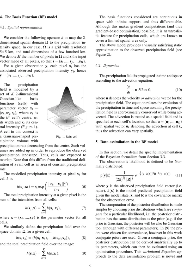
Fig. 1. Rain cell The precipitation
field is modelled by a set of K 2-dimensional Gaussian-like basis functions (cells) with parameter vector xk =
(ck,wk,rk), where ck is the kth cell’s centre, wk its width and rk its cen-tral intensity (Figure 1). A cell in this context is a Gaussian-shaped pre-cipitation volume with
precipitation rate decreasing from the centre. Such vol-umes are added up in order to reproduce the observed precipitation landscape. Thus, cells are expected to overlap. Note that this differs from the traditional defi-nition of a rain cell as an area of constant precipitation rate.
The modelled precipitation intensity at pixel sj for cell k is: h(sj,xk) =rkexp kc k−xjk2 2wk (6) The total precipitation intensity at a given pixel is the sum of the intensities from all cells:
h(sj,x) = K
∑
k=1
h(sj,xk), (7) where x= (x1, ...,xK) is the parameter vector for all cells.
We similarly define the precipitation field over the space domainΩfor a given cell:
h(s,xk) = (h(s1,xk), ...,h(sM,xk)), (8) and the total precipitation field over the image:
h(s,x) =
K
∑
k=1
h(s,xk). (9)
The basis functions considered are continuous in space with infinite support, and thus differentiable. Although this makes gradient computations (and thus gradient-based optimisation) possible, it is an unrealis-tic feature for precipitation cells, which are known to cover a limited spatial area only.
The above model provides a visually satisfying static approximation to the observed precipitation field (see Figure 2).
4.2. Dynamics
The precipitation field is propagated in time and space according to the advection equation:
∂h
∂t +u.∇h≈0, (10)
where u denotes the velocity or advection vector for the precipitation field. The equation relates the evolution of the precipitation in time and space assuming the precip-itation field is approximately conserved while being ad-vected. The advection is treated as a spatial field and is specified at each cell’s location, so that u= (u1, ...,uK) with spatial vector uk denoting the advection at cell k; thus the advection can vary spatially.
5. Data assimilation in the BF model
In this section, we detail the specific implementation of the Bayesian formalism from Section 3.3.
The observation’s likelihood is defined to be Nor-mally distributed: p(y|x) = 1 (2π)M2 |R| 1 2 e−12(y−h(x))TR−1(y−h(x)) (11)
where y is the observed precipitation field vector (i.e. radar), h(x) is the model predicted precipitation field given the model state, x, and R is the covariance matrix for the observation error.
The computation of the posterior distribution is made simpler by choosing prior distributions which are
conju-gate for a particular likelihood, i.e. the posterior
distri-bution has the same distridistri-bution as the prior (e.g. if the prior is Gaussian, the posterior will be also be Gaussian too, although with different parameters). In [9] the pri-ors were chosen for convenience, however in this work conjugate priors are used. Given a conjugate prior, the posterior distribution can be derived analytically up to its parameters, which can then be evaluated using an optimisation procedure. This variational Bayesian ap-proach to the data assimilation problem is novel and
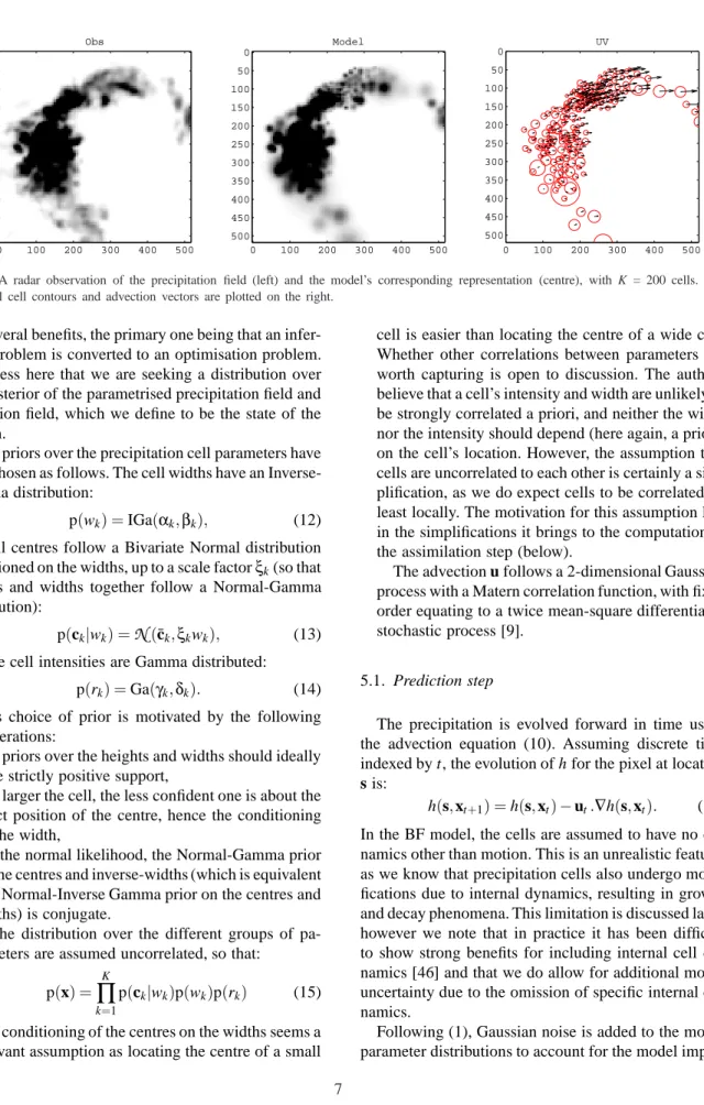
Obs t 0 100 200 300 400 500 0 50 100 150 200 250 300 350 400 450 500 Model 0 100 200 300 400 500 0 50 100 150 200 250 300 350 400 450 500 0 100 200 300 400 500 0 50 100 150 200 250 300 350 400 450 500 UV
Fig. 2. A radar observation of the precipitation field (left) and the model’s corresponding representation (centre), with K = 200 cells. The principal cell contours and advection vectors are plotted on the right.
has several benefits, the primary one being that an infer-ence problem is converted to an optimisation problem. We stress here that we are seeking a distribution over the posterior of the parametrised precipitation field and advection field, which we define to be the state of the system.
The priors over the precipitation cell parameters have been chosen as follows. The cell widths have an Inverse-Gamma distribution:
p(wk) =IGa(αk,βk), (12) the cell centres follow a Bivariate Normal distribution conditioned on the widths, up to a scale factorξk(so that centres and widths together follow a Normal-Gamma distribution):
p(ck|wk) =
N
(¯ck,ξkwk), (13) and the cell intensities are Gamma distributed:p(rk) =Ga(γk,δk). (14) This choice of prior is motivated by the following considerations:
– The priors over the heights and widths should ideally have strictly positive support,
– The larger the cell, the less confident one is about the exact position of the centre, hence the conditioning on the width,
– For the normal likelihood, the Normal-Gamma prior on the centres and inverse-widths (which is equivalent to a Normal-Inverse Gamma prior on the centres and widths) is conjugate.
The distribution over the different groups of pa-rameters are assumed uncorrelated, so that:
p(x) =
K
∏
k=1
p(ck|wk)p(wk)p(rk) (15) The conditioning of the centres on the widths seems a relevant assumption as locating the centre of a small
cell is easier than locating the centre of a wide cell. Whether other correlations between parameters are worth capturing is open to discussion. The authors believe that a cell’s intensity and width are unlikely to be strongly correlated a priori, and neither the width nor the intensity should depend (here again, a priori) on the cell’s location. However, the assumption that cells are uncorrelated to each other is certainly a sim-plification, as we do expect cells to be correlated, at least locally. The motivation for this assumption lies in the simplifications it brings to the computation in the assimilation step (below).
The advection u follows a 2-dimensional Gaussian process with a Matern correlation function, with fixed order equating to a twice mean-square differentiable stochastic process [9].
5.1. Prediction step
The precipitation is evolved forward in time using the advection equation (10). Assuming discrete time indexed by t, the evolution of h for the pixel at location s is:
h(s,xt+1) =h(s,xt)−ut.∇h(s,xt). (16) In the BF model, the cells are assumed to have no dy-namics other than motion. This is an unrealistic feature, as we know that precipitation cells also undergo modi-fications due to internal dynamics, resulting in growth and decay phenomena. This limitation is discussed later, however we note that in practice it has been difficult to show strong benefits for including internal cell dy-namics [46] and that we do allow for additional model uncertainty due to the omission of specific internal dy-namics.
Following (1), Gaussian noise is added to the model parameter distributions to account for the model
imper-fections. The cell heights and widths are left unchanged in mean but their covariances increase. The centres are modified according to the following:
p(ct+1|wt+1) =
N
(¯ct+1,Σct+1) (17)whereΣct+1 is the full diagonal covariance matrix for
the centres, i.e.Σct+1(k,k) =ξk,t+1wk,t+1, and
¯ct+1=¯ct+∆tut (18)
Σct+1 =Σct+ (∆t)
2Σ
ut+Qt (19)
Similarly to the widths and heights, the advection ut is assumed constant during the prediction. This is a realistic assumption at the time scales considered, where the evolution of the precipitation field is faster than that of the advection field. Again, a small amount of system error is added to reflect the inaccuracies in the model’s dynamics.
5.2. Assimilation step
The model described thus far is able to model a pre-cipitation field and propagate it through time in a gener-ative manner that can be used for simulation purposes. For it to work in a forecasting context, it needs to be tied to the underlying real process via real-time ob-servations. Section 3 described the general concepts of Bayesian data assimilation, and the need for some nu-merical method in order to evaluate the posterior distri-bution of the variable of interest. The initial model de-veloped by [9] used a maximum a posteriori method to determine the optimal state x∗, and a Laplace approx-imation about x∗to estimate the posterior uncertainty via the covariance matrix.
The maximum a posteriori method consists of find-ing the value x∗ of x which maximises the posterior probability (or, as is usually done in practice, the neg-ative logarithm of the posterior probability). The priors on the centres, widths and heights were chosen to be convenient to compute and the posterior up to a normal-ising constant was computed analytically; the optimum was determined using the scaled conjugate gradient op-timisation method [42].
The Laplace approximation (see for example [36]) uses the fact that at its maximum, the log-posterior can be expanded using Taylor expansion as follow:
ln p(x)≈ln p(x∗)−1
2(x−x
∗)TH(x−x∗) (20) where H is the Hessian of ln p at point x∗. Then, if we denote Z the, typically unknown, normalising constant, p can be approximated at point x∗by the Gaussian dis-tribution: q(x) = 1 Z exp −1 2(x−x ∗)TH(x−x∗) . (21)
The Laplace assumption is only valid about the maxi-mum in the posterior, it is important for accurate results to ensure x∗is as close as possible to this maximum. As the number of cells considered increases, reaching the required accuracy becomes computationally expensive, and slows down the model considerably. The approx-imation is also a local one, and is likely to underesti-mate the posterior variance, especially if the posterior distribution is multi-modal, although we have not found strong evidence for multi-modal posteriors in this prob-lem.
In order to improve the assimilation of radar data, a new approach is presented here which relies on Varia-tional Bayesian techniques. VariaVaria-tional Bayes was in-troduced by [27] in a paper which showed that the true posterior distribution can be approximated by a Gaus-sian distribution using a deterministic algorithm. The method can be applied to other types of distributions, and involves minimising the Kullback-Leibler (KL) di-vergence between the true posterior and some simpler, parametric, approximating distribution, for which pa-rameters are estimated. The KL divergence, or relative entropy, between the posterior p and the approximating distribution q, is defined as follows:
KL(qkp) =− Z q(xt|Yt) ln p(xt|Yt) q(xt|Yt) dx (22) Given the conjugate nature of the priors chosen, the q distribution has the same structure as the prior. Given the prior (eq. 15) and the likelihood (eq. 11), the ex-pression for p(xt|Yt)can be obtained, up to a constant, by applying Bayes’ rule (Eq. 4), leading to:
KL(qkp)∝− Z q(xt|Yt) ln p(yt|xt)p(xt|Yt−1) q(xt|Yt) dx (23) Expanding this yields:
KL(pkq)∝− ln p(yt|xt) q(xt|Yt) − lnp(xt|Yt−1) q(xt|Yt) q(xt|Yt) (24)
where the cross-entropy of p with respect to q is defined as: ln p(x) q(x) =− Z q(x) ln p(x) dx (25) The likelihood term arising from the new radar im-age being assimilated expands, after computation, and omitting the time index for readability, to:
− ln p(y|x) q(x|Y) = 1 2σ2 M
∑
j=1 N∑
k=1 Ek,j−yj !2 − N∑
k=1 Ek,j 2 + N∑
k=1 Fk,j (26) with Ek,j= γk δk(1+ξk) 1+(¯ck−sj) T(¯c k−sj) 2βk(1+ξk) −αk (27) and Fk,j= γk(γk+1) δ2 k(1+2ξk) 1+(¯ck−sj) T(¯ck−s j) βk(1+2ξk) −αk (28) Further computation leads to the following results for the prior term:− lnp(x|Y) q(x|Y) q(x|Y) = N
∑
k=1 γklnδk−γ′klnδ′k−ln Γ(γk) Γ(γ′ k) + (γk−γ′k) [Ψ(γk)−lnδk]−γk 1−δ ′ k δk +αklnβk−α′klnβ′k−ln Γ(αk) Γ(α′ k) + (αk−α′k) [Ψ(αk)−lnβk]−αk 1−β ′ k βk +lnξ ′ k ξk +ξξk′ k + 1 2ξ′k αk βk (¯ck−¯c′k)T(¯ck−¯c′k) −N 2 (29)in which the prime is used to distinguish the prior pa-rameters from the equivalent papa-rameters in the posterior. TheΓandΨoperators are the standard Gamma func-tion and its first derivative (Digamma) . We omit the full derivation of these results which requires a series of non-trivial integrals. These will be made available in a future report. The main point to note is that the use of the variational Bayes framework allows us to repose the estimation of the posterior distribution by a minimisa-tion of Equaminimisa-tion 24. The minimisaminimisa-tion is achieved using a scaled conjugate gradient algorithm [3; 42]. Since the q distribution is an approximation to the posterior dis-tribution we are able to take relatively few optimisation steps and still have reasonable estimates of the poste-rior uncertainty about the locations of the precipitation cells in particular, which is crucial in obtaining realistic estimates of the advection field, and our uncertainty in this.
5.3. Forecast
The predicted distribution at a given lag L is given by:
p(xt+L|Yt) = Z
p(xt+L|xt)p(xt|Yt)dxt. (30) Since the model is assumed Markov, the predicted dis-tribution in the integral factorises as the product of all intermediate predicted estimates, giving:
p(xt+L|Yt) = Z .. Z p(xt+L|xt+L−1). . .p(xt+1|xt) p(xt|Yt)dxL−1. . .dxt. (31) Although this formulation allows for the full distribu-tion of the state to be forecast forward in time according to Equation (1), it relies heavily on a good specification of the model error. Because this model error has been chosen Gaussian, which we know is unrealistic, an alter-native approach based on Monte Carlo approximation is preferred. A number of realisations are sampled from the state’s distribution p(xt|Yt)and propagated to time t+L using the model. The forecast distribution is then approximated by the ensemble of forecasts, from which statistics can be estimated. This method is expected to better capture the variability introduced by the model and compensate for the crude error model chosen.
The forecast is obtained by propagating the cells lin-early given their initial advection estimate. This is a very simple advection model, and it is expected to give rea-sonable forecasts at short times only (up to 1h), where the linear approximation holds. At longer lead times, a better forecasting scheme would have the cells propa-gated according to the estimated advection at their pre-dicted location, rather than at their initial location. This has not been been implemented in the current work, but will be the primary focus of upcoming developments. 5.4. Extensions to the model
In order to apply the model to real data, a number of additional extensions to the model in [9] were required. It is beyond the scope of this paper to discuss these in detail, but it is worth mentioning them:
– Support for the deletion of “dead” cells (cells that have collapsed or moved out of the observable area). – Support for the detection of new cells (cells that have appeared as a result of in situ convective development or that have been advected into the observable area). – Localisation of each cell’s precipitating area: by de-sign, the cells have infinite support. It is thus im-portant to limit their effect to a certain radius from
the centre. A cut-off of 0.8 mm.h−1 is applied, be-yond which the effect of the cell is ignored. This also speeds up the computation considerably.
These extensions make is possible to run the model on large radar images, over long time periods.
6. Preliminary results
As a sanity check, we first test the ability of the model to correctly locate a single precipitation cell, on simu-lated data. The data is generated by propagating a single precipitation cell with constant, horizontal advection of 6 m.s−1. The cell is 42 km wide and its central inten-sity is 33 mm.h−1. Observations are taken every 900 s and corrupted with Gaussian white noise with variance 4.0 mm2.h−2. The noise is applied locally, i.e. only to those pixels where the precipitation rate exceeds some threshold (0.8 mm.h−1). This is believed to be a real-istic noise model for simulated radar-like data, since it is empirically observed that radar is usually well able to identify geographical regions without precipitation, with the errors occurring mainly in the regions where precipitation is detected [39]. Other noise models were tested (global additive noise and multiplicative noise), but they did not lead to any significant differences in the results.
Fig. 3. Single precipitation cell: movement in time – The top row shows the predicted precipitation cell (top), the observed precipita-tion cell (middle) and the assimilated precipitaprecipita-tion cell (bottom) at 3 different times: initial guess (left), assimilation (centre) and end of forecast (right).
The cell parameters are estimated over 180 time steps (equating to 45 hours), and then forecast over 12 steps (3 hours). The initial variances over the centres, widths and heights are set to 10.0, representing weak knowledge
of the initial state at the start of the assimilation. The propagation error variance (also known as the model error component) is set to 25 km2.h−1for the centres, 0.1 mm2.h−1for the central intensity, 0.1 km2.h−1for the cell widths and 1.6 m2.s−2.h−1 for the advection field. These priors are chosen to be characteristic of the typical model errors we might expect for real data, and have been derived by analysis of radar image sequences. Figure 3 shows the predicted, observed and assimi-lated cells from the idealised model at 3 different times. At the end of the assimilation period, the cell is prop-agated forward in time using the last estimate of the parameters. There is no noticeable difference between the cell’s characteristics at the end of the forecast and the observed cell, which confirms the model managed to track the “true” cell on this very simple validation example.
7. Results on real data
In order to test the model on real data, the model is run against radar observations from a convective pre-cipitation event in the summer of 2006 and to contrast on a frontal precipitation event in the winter of 2005. Both experiments use NIMROD radar data provided by the UK Met Office, accessed through the British Atmo-spheric Data Centre [54].
The observations were pre-processed using a Gaus-sian filter with radius 10 km to improve the estimation of the model precipitation field. The spatial domain was restricted to 500×500 km (100×100 pixels) and the model was run with a limited number of 250 cells, in or-der to keep computation times sufficiently low (less than 5 minutes per observation processed). Furthermore, the optimisation of the KL divergence was limited to 200 iterations, which proved sufficient in practice to achieve a good fit of the posterior distribution while remaining computationally efficient.
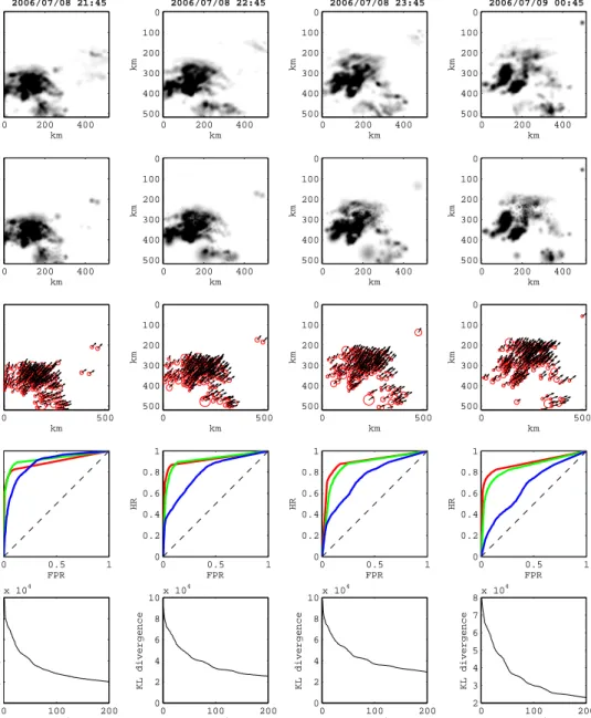
The assimilation was carried out over a sequence of 672 observations, taken every 15 minutes, which amounts to a weeks worth of data (168 hours). Figure 5 show the state of the model for the convective event, af-ter about 67 hours of data (270 observations) have been assimilated. 4 hourly estimates are shown. This corre-sponds to a peak in the complexity of the precipitation field, and thus to a peak in the Root Mean Square Er-ror (RMSE) with respect to the mean of the posterior distribution, as shown in Figure 8. Reading from top to bottom Figure 5 shows: the radar observations of pre-cipitation, the corresponding estimated precipitation af-ter assimilation of the observed radar, the cell contours
2006/07/08 21:45 km km 0 200 400 0 100 200 300 400 500 km km 0 200 400 0 100 200 300 400 500 0 500 0 100 200 300 400 500 km km 0 0.5 1 0 0.2 0.4 0.6 0.8 1 FPR HR 0 100 200 0 2 4 6 8 10x 10 4 KL divergence Iteration 2006/07/08 22:45 km km 0 200 400 0 100 200 300 400 500 km km 0 200 400 0 100 200 300 400 500 0 500 0 100 200 300 400 500 km km 0 0.5 1 0 0.2 0.4 0.6 0.8 1 FPR HR 0 100 200 0 2 4 6 8 10x 10 4 KL divergence Iteration 2006/07/08 23:45 km km 0 200 400 0 100 200 300 400 500 km km 0 200 400 0 100 200 300 400 500 0 500 0 100 200 300 400 500 km km 0 0.5 1 0 0.2 0.4 0.6 0.8 1 FPR HR 0 100 200 0 2 4 6 8 10x 10 4 KL divergence Iteration 2006/07/09 00:45 km km 0 200 400 0 100 200 300 400 500 km km 0 200 400 0 100 200 300 400 500 0 500 0 100 200 300 400 500 km km 0 0.5 1 0 0.2 0.4 0.6 0.8 1 FPR HR 0 100 200 2 3 4 5 6 7 8x 10 4 KL divergence Iteration
Fig. 4. Convective event – This plot shows the evolution of the observed (a) and estimated (b) rainfall over a 4-hour period (from left to right). The main cells and their associated advection are shown on row (c). ROC curves for a fixed threshold of 1 mm.h-1are shown on row
(d) for 3 different forecast lead times: 30 min (top curve), 60 min (middle curve) and 180 min (bottom curve). The dashed line correspond to a non informative forecast (no skill). Row (e) shows the optimisation of the KL divergence over 200 optimisation steps.
along with their advection vectors (only the major cells are displayed for clarity), the ROC curves for a precip-itation threshold Rmin=1 mm.h−1 with 3 curves cor-respond, from the upper one to the lower one, to the forecasts at t+30 min, t+60 min and t+180 min, and, on the bottom row, the KL convergence curves for each of the 4 time steps considered.
The quality of the probabilistic forecasts was assessed based on [2]. At each 15 minute time step, 100 real-isations of the stochastic model were generated from the parameters posterior distribution and then propa-gated forward in time, to provide an Monte Carlo (or large ensemble) estimate of the probability distribution of the precipitation rates over the region at times from t+15min to t+180 min. Given a precipitation threshold
Rmin, the model is considered to detect rain at a given location if at least N forecasts out of the 100 predict rain exceeding Rminat that location. The same threshold is applied to the observed rainfall and the Hit Rate (ratio of correctly detected wet locations) is plotted against the False Prediction Rate (ratio of incorrectly detected dry locations). The ROC curve is generated by having N vary from 0 to 100. Ideally the all forecasts for a given
N will have 100% hit rates, and zero false alarms,
cor-responding to a line along the top of the plot. A random forecast should plot along the diagonal line. Thus a per-fect probabilistic forecast will result in the area between the curve and the diagonal [0,1] being 0.5, whereas an area close to zero indicates poor skill (zero being equiv-alent to a random forecast). The area under the curve is computed as the sum of the “slices” between any two sequential points ak−1and akon the curve, joined by a straight line (trapezoidal Riemann sum). The total area is thus given by:
1 2 N
∑
k=2 [FPR(ak)−FPR(ak−1)]× [HR(ak) +HR(ak−1)] (32)Figure 5 shows that after seeing 67 hours of data the model is able to assimilate the radar data to estimate the precipitation field while also jointly estimate advection vectors for the precipitation field. It can be noticed that the appears somewhat ‘spotty’ in some parts. We be-lieve this relates to the partial optimisation of the KL-divergence; as can be seen from the bottom line of the figure, the KL-divergence has not converged full in the optimisation, much like the 3D VAR cost function is only partially optimised in classical data assimilation. This might also be related to the convective nature of the event, with the birth / death processes of the ‘pre-cipitation cells’ making it very difficult for the model
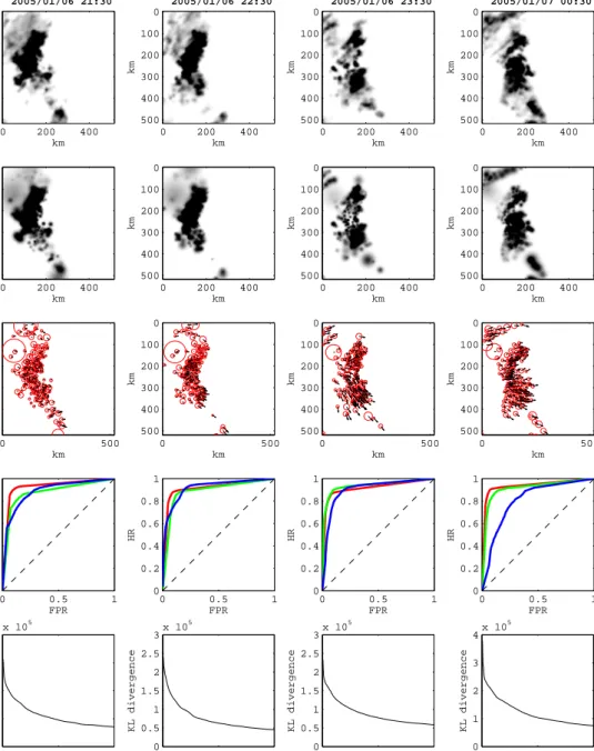
to track specific precipitation features, and resulting in cells being frequently added and removed. The advec-tion vectors show a clear storm moadvec-tion from south-west to north-east, but there are small variations in the advec-tion over space, which are likely to reflect differential development and possibly steering of the precipitation field. The ROC curves (4th line) for the four times show that at moderate lead times t+30 min and t+60 min the probabilistic predictions have considerable skill, how-ever for this convective event at t+180 min the skill is much reduced, but still considerably better than random. Figure 7, shows the same information as Figure 5 but for the January 2005 frontal rainfall event, starting this time after 60 hours of data (240 observations) have been assimilated. We note that the assimilation method quickly converges and thus could be shown after only 2 cycles of assimilation and would show similar results. We again see a good fit the the assimilated precipita-tion field, but again note a problem with some rather ‘spotty’ behaviour in the assimilated estimate of pre-cipitation. This problem appears to be most severe in region with strong dynamic changes to the advected precipitation field. The advection vectors from this ex-ample show rather complex structure. Initially this was felt to be a problem with the model, however it appears that there is strong apparent differential advection in this storm, probably related to embedded precipitation elements within the frontal zone, particularly early in the time window show here. At the later times the ad-vection seems more uniform across the domain consid-ered. In contrast to the convective scenario the the ROC curves show that forecast skill is retained far longer, with quite respectable skill shown even at t+180 min as might be expected in the more strongly dynamically forced, larger scale processes typical in frontal precip-itation. Finally we note that for computational reasons we truncated the optimisation of the KL-divergence at 200 iterations, but it is clear that the system has not fully converged.
8. Discussion
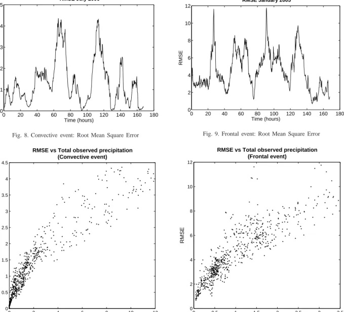
To further evaluate the performance of the model, two statistical validation methods have been applied. The quality of the assimilation was validated using the traditional Root Mean Square Error (RMSE) while the forecasting ability was assessed using ROC curve based verification statistics over the full assimilation window. The RMSE measures the average distance (over the spatial domain) between the model’s estimate and the ‘true’observed precipitation field as measured by the
2005/01/06 21:30 km km 0 200 400 0 100 200 300 400 500 km km 0 200 400 0 100 200 300 400 500 0 500 0 100 200 300 400 500 km km 0 0.5 1 0 0.2 0.4 0.6 0.8 1 FPR HR 0 100 200 0 1 2 3 4 x 10⁵ KL divergence Iteration 2005/01/06 22:30 km km 0 200 400 0 100 200 300 400 500 km km 0 200 400 0 100 200 300 400 500 0 500 0 100 200 300 400 500 km km 0 0.5 1 0 0.2 0.4 0.6 0.8 1 FPR HR 0 100 200 0 0.5 1 1.5 2 2.5 3 x 10⁵ KL divergence Iteration 2005/01/06 23:30 km km 0 200 400 0 100 200 300 400 500 km km 0 200 400 0 100 200 300 400 500 0 500 0 100 200 300 400 500 km km 0 0.5 1 0 0.2 0.4 0.6 0.8 1 FPR HR 0 100 200 0 0.5 1 1.5 2 2.5 3 x 10⁵ KL divergence Iteration 2005/01/07 00:30 km km 0 200 400 0 100 200 300 400 500 km km 0 200 400 0 100 200 300 400 500 0 500 0 100 200 300 400 500 km km 0 0.5 1 0 0.2 0.4 0.6 0.8 1 FPR HR 0 100 200 0 1 2 3 4 x 10⁵ KL divergence Iteration
Fig. 6. Frontal event – This plot shows the evolution of the observed (a) and estimated (b) rainfall over a 4-hour period (from left to right). The main cells and their associated advection are shown on row (c). ROC curves for a fixed threshold of 1 mm.h-1are shown on row (d) for 3 different forecast lead times: 30 min (top curve), 60 min (middle curve) and 180 min (bottom curve). The dashed line correspond to a non informative forecast (no skill). Row (e) shows the optimisation of the KL divergence over 200 optimisation steps.
0 20 40 60 80 100 120 140 160 180 0 1 2 3 4 5 RMSE July 2006 RMSE Time (hours)
Fig. 8. Convective event: Root Mean Square Error
0 20 40 60 80 100 120 140 160 180 0 2 4 6 8 10 12 Time (hours) RMSE RMSE January 2005
Fig. 9. Frontal event: Root Mean Square Error
0 2 4 6 8 10 12 x 104 0 0.5 1 1.5 2 2.5 3 3.5 4 4.5
RMSE vs Total observed precipitation (Convective event)
Total observed precipitation (mm.h−1)
RMSE
Fig. 10. Scatter plot of RMSE vs Total observed precipitation (July 2006) – The Root Mean Square Error between the estimated rainfield and the observation is plotted against the total observed precipitation for each of the 672 observations in the convective experiment.
0 0.5 1 1.5 2 2.5 3 3.5 x 10⁵ 0 2 4 6 8 10 12
RMSE vs Total observed precipitation (Frontal event)
Total observed precipitation (mm.h−1)
RMSE
Fig. 11. Same as Figure 10 for the frontal event (January 2005).
radar. Figures 8 and 9 show the evolution of the RMSE in time over the assimilation period. The assimilation appears to give better results for the convective event (Figure 8) than for the frontal event (Figure 9). This is to be related to the spatial complexity of the precipitation field, which is greater in the winter event, probably due to the higher overall rain rates, and the greater part of the domain covered by precipitation compared to the summer event. Figures 10 and 11 show scatter plots of the RMSE against the total observed precipitation
(summed over the spatial domain) for the convective and frontal cases respectively. This confirms, in both cases, the correlation between the complexity of the precipitation field and the quality of the corresponding estimate.
For both cases the same, limited, number of cells (250) was used which is probably not overly realistic. In practice it would be very desirable to be able to estimate an appropriate complexity for the model, which could adapt to the complexity of the observations. This was
0 50 100 150 200 250 300 350 400 450 500 0 2 4 6 8 10 12 14 16 18 20 Number of cells RMSE 0 50 100 150 200 250 300 350 400 450 5000 10 20 30 40 50 60 70 80 90 100 Time (s)
Effect of number of cells on RMSE/initialisation time
Fig. 12. Trade off between number of cells and initialisation speed. This plot shows the effect of the number of cells used on the quality of the fit and computation time. The dashed curve (left y-axis) is the root mean square error between the observation and the model’s estimated rainfall field. The solid curve (left y-axis) is the initialisation time in seconds.
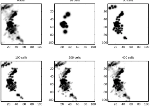
Radar 20 40 60 80 100 20 40 60 80 100 100 cells 20 40 60 80 100 20 40 60 80 100 10 cells 20 40 60 80 100 20 40 60 80 100 200 cells 20 40 60 80 100 20 40 60 80 100 50 cells 20 40 60 80 100 20 40 60 80 100 400 cells 20 40 60 80 100 20 40 60 80 100
Fig. 13. Fit to the data with increasing number of cells. This plot shows the model’s realisation as the number of cells increases. The actual observation is shown in the top left corner.
not implemented in this version of the code but we be-lieve that it might be possible to incorporate a ‘sparsity’ prior in the model, in a similar manner to the treatment of the relevance vector machine [53]. The model is this better able to represent the simple, localised precipita-tion patterns which make up most of the convective data compared to the complex, diffuse precipitation patterns from the winter data. This also explains the consider-able variations in the RMSE for each event, where quiet, dry(er) periods alternate with stormy phases.
The fit to the data can be improved by increasing the number of cells, but this comes at the price of computa-tional time, which needs to be kept below the time incre-ments between two observations. Figure 12 shows how the Root Mean Square Error (dashed line) decreases as more and more cells are allowed into the model. Com-putation time (solid line) increases almost linearly with the number of cells. A limit of 250 cells is sufficient to discard more than 90% of the misfit while keeping computation time below 30 seconds. Figure 13 shows how the fit to the data improves as the number of cells increases. In this work the complexity was chosen to keep the computational time to less than 5 minutes per assimilation cycle on a 1.6 GHz single core desktop PC. It is theoretically possible to parallelise many of the computations in the algorithm to exploit future multi-core machines or dedicated parallel architectures if the method were taken into operational use.
The RMSE results only tell half the story, since this
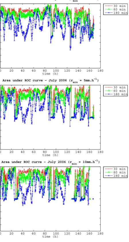
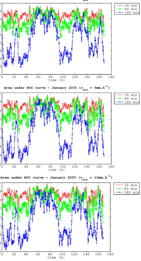
model is designed to be probabilistic. The most widely used diagnostic for probabilistic models in precipitation forecasting is the area under the ROC curve. Figures 14 and 15 show the evolution of the area under the ROC curve as a function of time. Results are plotted, from top to bottom, for the 3 precipitation intensity thresholds (1, 5, and 10 mm.h−1). Each plot shows the evolution of the area for the 3 forecast lead times (t+30 min, t+60 min and t+180 min).
Note that the absence of rain (or heavy rain) during some periods can result in erroneous ROC curves. If no rain is observed, the Hit Rate cannot be computed (di-vision by zero). This results in missing points on the curve as can be seen on the bottom plot around t=130h. In the case where no rain cell is left in the model (as a result from a dry observation being assimilated), all of the model’s realisations will predict a dry forecast, hence all points will coincide with the bottom left cor-ner (HR=FAR=0), resulting in a curve aligned with the diagonal and an area of exactly 0.5. Several such cases can be observed in the two lower plots, where the detection thresholds is higher. These cases should ide-ally be discarded as they don’t give a correct account of the model’s prediction skill.
Figure 15 shows similar information to Figure 14 for the frontal event. It can be observed that the prediction skill varies more smoothly that in the convective case, due to the larger scale and slower nature of the pre-cipitative developments. Two regimes can be identified,
0 20 40 60 80 100 120 140 160 180 0 0.1 0.2 0.3 0.4 0.5 0.6 0.7 0.8 0.9 1 time (h)
Area under ROC curve
Area under ROC curve − July 2006 (r
min = 1mm.h −1 ) 30 min 60 min 180 min 0 20 40 60 80 100 120 140 160 180 0 0.1 0.2 0.3 0.4 0.5 0.6 0.7 0.8 0.9 1 time (h)
Area under ROC curve
Area under ROC curve − July 2006 (r
min = 5mm.h −1 ) 30 min 60 min 180 min 0 20 40 60 80 100 120 140 160 180 0 0.1 0.2 0.3 0.4 0.5 0.6 0.7 0.8 0.9 1 time (h)
Area under ROC curve
Area under ROC curve − July 2006 (r
min = 10mm.h −1 ) 30 min 60 min 180 min
0 20 40 60 80 100 120 140 160 180 0.1 0.2 0.3 0.4 0.5 0.6 0.7 0.8 0.9 1 time (h)
Area under ROC curve
Area under ROC curve − January 2005 (r
min = 1mm.h −1 ) 30 min 60 min 180 min 0 20 40 60 80 100 120 140 160 180 0.2 0.3 0.4 0.5 0.6 0.7 0.8 0.9 1 time (h)
Area under ROC curve
Area under ROC curve − January 2005 (r
min = 5mm.h −1 ) 30 min 60 min 180 min 0 20 40 60 80 100 120 140 160 180 0.2 0.3 0.4 0.5 0.6 0.7 0.8 0.9 1 time (h)
Area under ROC curve
Area under ROC curve − January 2005 (r
min = 10mm.h −1 ) 30 min 60 min 180 min
t = 10h t = 20h t = 30h t = 40h t = 50h t = 60h t = 70h t = 80h
t = 90h t = 100h t = 110h t = 120h t = 130h t = 140h t = 150h t = 160h
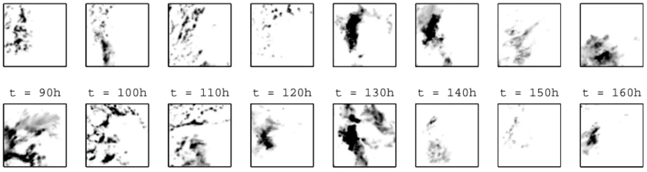
Fig. 16. Evolution of the rainfall field during the frontal event (January 2005, 10h snapshots).
one in which the prediction skill decreases quickly (t=0-40, t=100-120, t=140-160) and one where the predic-tion skill is retained much longer, to the point that even 180min forecasts still show some good skill (t=60-90, t=120-140).
Qualitative analysis has shown that these two regimes can be related to the nature of the observed rainfall field. Figure 16 displays the observed rainfall field at 10h intervals. Heavily clustered fields of high precipi-tation intensity seem to result in good forecasts while sparse, localised precipitation fronts correspond to poor forecasts. This could be due to the linear forecasting scheme, which is likely to perform better when the rain cells are clustered as this ensures their advection field is smooth. Another possible explanation is the assump-tion, in advection-based forecasts, that motion is the primary factor of change, and that internal development (growth/decay) can be neglected. It is clear that dissipa-tion phenomena are less noticeable, in propordissipa-tion, for large areas of intense precipitation than for smaller iso-lated cells.
Figures 17 and 18 summarise the distributions, for the whole experiment, of the areas under the ROC curve. As expected, the model skill decreases on average as the forecast lead time increases, with very little skill in any of the forecasts after 3 hours. This is due partly to the simplicity of the precipitation field representation, and partly to the linear nature of the forecast scheme applied. Each cell is advected linearly given the advec-tion at its centre, an assumpadvec-tion which remains rele-vant only for shorter forecast lead times. A better ad-vection scheme would involve projecting the adad-vection field onto a fixed grid and advecting the cells accord-ing to the advection at their future location rather than at their initial location. At short time scales, particular at t+30 min the model has more skill when forecasting
heavy precipitation (>10 mm.h−1) than light precipita-tion (1 mm.h−1). This is a useful feature, since for most flood forecasting applications the heavy precipitation is the most important to predict well. This is a common feature of many advection models, since the heavier precipitation tends to be more temporally persistent.
Figure 19 shows the variogram [12; 37] and for the observed and assimilated rainfall field (top left) at time t=70 h into the experiment. Variograms for the corre-sponding forecasts from times t-30 min (bottom left), t-60 min (top right) and t-180 min (bottom right) are shown, along with 4 random sample forecast realisa-tions. The predicted rainfall field at +30 min provides a visually satisfying estimate of the observed rainfall field, with sufficient detail. The +60 min forecast still captures the overall precipitation structure, although in-accurately predicts rain in the south-eastern part of the domain, most certainly due to previous observed pre-cipitation which has since then dissipated. The +180 min forecast is rather poor, due to the linear advection scheme which does not maintain, at longer lead times, the cohesion of the field (as observed from the “spotty” nature of the forecast). However, the variograms show that the model is able to retain the overall structure at short scales (<100 km), but quickly diverges at larger scales in that example.
9. Conclusions
This paper presents a new probabilistic data assim-ilation algorithm which can be applied to nowcasting using a simple advection based precipitation forecast-ing model. The algorithm has several desirable features, in particular the ability to estimate the posterior distri-bution of the model state using optimisation methods, which provides control over the computational
com-1 5 10 −0.5 −0.4 −0.3 −0.2 −0.1 0 0.1 0.2 0.3 0.4 0.5 ROC area Detection threshold (mm.h−1 ) 30 min forecast 1 5 10 −0.5 −0.4 −0.3 −0.2 −0.1 0 0.1 0.2 0.3 0.4 0.5 ROC area Detection threshold (mm.h−1 ) 60 min forecast 1 5 10 −0.5 −0.4 −0.3 −0.2 −0.1 0 0.1 0.2 0.3 0.4 0.5 ROC area Detection threshold (mm.h−1 ) 180 min forecast
Fig. 17. Convective event: ROC areas
1 5 10 −0.5 −0.4 −0.3 −0.2 −0.1 0 0.1 0.2 0.3 0.4 0.5 ROC area Detection threshold (mm.h−1 ) 30 min forecast 1 5 10 −0.5 −0.4 −0.3 −0.2 −0.1 0 0.1 0.2 0.3 0.4 0.5 ROC area Detection threshold (mm.h−1 ) 60 min forecast 1 5 10 −0.5 −0.4 −0.3 −0.2 −0.1 0 0.1 0.2 0.3 0.4 0.5 ROC area Detection threshold (mm.h−1 ) 180 min forecast
Fig. 18. Frontal event: ROC areas
plexity. While the intial derivation is quite mathemati-cally demanding, the implementation can be employed within any optimisation framework, which forms the basis for most traditional variational assimilation meth-ods.
The new method is tested on two large events char-acterised by convective and frontal dominated rainfall. The results show the model is numerically robust, al-though further testing is necessary to assess its appli-cability to operational nowcasting . The ROC curves show probabilistic skill at all forecast horizons, but it is clear that skill is lost rapidly, which is typical of such advection / extrapolation based systems. Future work should ideally compare the results of the variational Bayes methods with other approaches. This would be greatly facilitated by a suit of standard test cases and diagnostics that could be agreed up by the nowcasting community to allow model and method comparison.
There are several areas in which the algorithm could be improved. Parallelisation would allow the algorithm to be optimised for more cycles resulting in an optimal KL-divergence based fit, and the number of cells used in the approximation to the precipitation field could also be increased. The inclusion of an automatic method to select the complexity of the model, using methods sim-ilar to those used in the relevance vector machine [53] would further improve the robustness and scaleability of the algorithm. The advection process representation is also rather crude and could be improved with a better representation of the advection field based on a fixed grid and non-linear forecasting methods. It must also be stated that the model, or propagation, error parameters have been set with reference to other studies and tuning on short data sequences and these are almost certainly not optimised. It would be possible to use the marginal
likelihood approximation, derived from the variational Bayes analysis to optimise these parameters as part of the data assimilation method, indeed these could be made adaptive since it is likely that the model error will be state dependent in this application.
More speculatively it would be interesting to attempt to include satellite imagery to track the evolution of the cloud field to better estimate the advection field where precipitation has yet to begin, but where clouds are present. Assimilation of other observation types, includ-ing doppler lidar and other more direct measurements of advection would further improve the estimation in the model. Further work could consider a hybrid approach that combines the knowledge of the physical system em-bodied in high resolution numerical models [15] but is sufficiently simple to be run on the short assimilation cy-cles required for short range forecasts. Since the model formulation is probabilistic and the uncertainty repre-sents the model uncertainty reasonably well, Bayesian model averaging could be applied to merge smoothly into a more physics based forecast at longer lead times, so long as the uncertainty on both were well charac-terised. It is the belief of the authors that more effort should be placed on accurately quantifying uncertainty than is currently the case in many forecasting activities. This paper provides a new mechanism for attempting to achieve this in the nowcasting context.
10. Acknowledgements
The authors would like to thank the UK Met Office for providing radar data free of charge via the British Atmospheric Data Centre [54], allowing this work to be carried out on real data. Some parts of this work
0 50 100 150 200 0 50 100 150 200 250 300 350 400 Lag (km) 2 γ Variograms Observed
Model (assimilated, mean)
Observation Model 0 50 100 150 200 0 50 100 150 200 250 300 350 400 Lag (km) 2 γ Variograms Sample 1 Sample 2 Sample 3 Sample 4 Sample 1 Sample 2 Sample 3 Sample 4 0 50 100 150 200 0 50 100 150 200 250 300 350 400 Lag (km) 2 γ Variograms Sample 1 Sample 2 Sample 3 Sample 4 Sample 1 Sample 2 Sample 3 Sample 4 0 50 100 150 200 0 50 100 150 200 250 300 350 400 Lag (km) 2 γ Variograms Sample 1 Sample 2 Sample 3 Sample 4 Sample 1 Sample 2 Sample 3 Sample 4
Fig. 19. Variograms of the observed and forecast precipitation fields (July 2006, t=70h). Variograms and rainfall fields correspond to observed and assimilated (top left), 30 min (bottom left), 60 min (top right) and 180 min (bottom right) forecasts. Four forecast realisations are plotted.
were funded by the EPSRC supported VISDEM project (EP/C005848/1).
References
[1] P. Alberoni, V. Ducrocq, G. Gregoric, G. Haase, I. Holleman, M. Lindskog, B. Macpherson, M. Nuret, A. Rossa, Quality and assimilation of radar data for NWP - a review, Tech. rep., COST-717 (2003).
[2] F. Atger, Verification of intense precipitation forecasts from single models and ensemble prediction systems, Nonlinear Processes in Geophysics 8 (2001) 401–417.
[3] C. Bishop, Neural Networks for Pattern Recognition, Oxford University Press, 1996.
[4] D. Bocchiola, R. Rosso, The use of scale recursive estimation for short term quantitative precipitation forecast, Physics and Chemistry of the Earth 31 (18) (2006) 1228–1239.
[5] N. Bowler, C. Pierce, A. Seed, STEPS: a probabilistic precipi-tation forecasting scheme which merges an extrapolation now-cast with downscaled NWP, Quarterly Journal of the Royal Meteorological Society 132 (2006) 2127–2155.
[6] K. Browning, A. Blyth, P. Clark, U. Corsmeier, C. Morcrette, J. Agnew, S. Ballard, D. Bamber, C. Barthlott, L. Bennett, et al., The Convective Storm Initiation Project, Bulletin of the American Meteorological Society 88 (12) (2007) 1939–1955. [7] A. Burton, P. O’Connell, Model based algorithms for short lead time nowcasting, Tech. Rep. 5.3, MUSIC project report (2003).
[8] V. Collinge, The development of weather radar in the UK, Wiley, 1987.
[9] D. Cornford, A Bayesian state space modelling approach to
probabilistic quantitative prediction forecasting, Journal of Hy-drology 288 (1-2) (2004) 92–104.
[10] P. Cowpertwait, P. O’Connell, A. Metcalfe, J. Mawdsley, Stochastic point process modelling of rainfall. I. Single-site fitting and validation, Journal of Hydrology 175 (1-4) (1996) 17–46.
[11] D. Cox, V. Isham, A simple spatial-temporal model of rainfall, Proceedings of the Royal Society of London A415 (1988) 317–328.
[12] N. Cressie, Statistics for Spatial Data, Wiley and Sons, 1993. [13] R. Deidda, Rainfall downscaling in a space-time multifractal framework, Water Resources Research 36 (7) (2000) 1779– 1794.
[14] M. Dixon, G. Wiener, Titan: Thunderstorm identification, tracking, analysis, and nowcasting - a radar-based methodol-ogy, Journal of Atmospheric and Oceanic Technology 10 (6) (1993) 785–797.
[15] J. M. Done, P. A. Clark, G. C. Craig, M. E. B. Gray, S. L. Gray, Mesoscale simulations of organised convection: Impor-tance of convective-equilibrium, Quarterly Journal of the Royal Meteorological Society 132 (2006) 737–756.
[16] A. Favre, A. Musy, S. Morgenthaler, Unbiased parameter es-timation of the Neyman–Scott model for rainfall simulation with related confidence interval, Journal of Hydrology 286 (1-4) (200(1-4) 168–178.
[17] U. Germann, I. Zawadzki, Scale-Dependence of the Pre-dictability of Precipitation from Continental Radar Images. Part I: Description of the Methodology, Monthly Weather Re-view 130 (12) (2002) 2859–2873.
[18] U. Germann, I. Zawadzki, Scale Dependence of the Predictabil-ity of Precipitation from Continental Radar Images. Part II: Probability Forecasts, Journal of Applied Meteorology 43 (1) (2004) 74–89.