Spatiotemporal Processes and Other Complex
Models
by Joon Ha Park
A dissertation submitted in partial fulfillment of the requirements for the degree of
Doctor of Philosophy (Statistics)
in the University of Michigan 2018
Doctoral Committee:
Professor Edward L. Ionides, Chair Associate Professor Yves A. Atchad´e Professor Aaron A. King
First and foremost, I would like to thank my advisor Professor Edward Ionides for his guidance and support throughout my PhD study. This work would not have been possible without the countless pieces of advice he offered. Whenever I inquired him about anything, he provided me with helpful feedback I very much needed. He has always guided my research with patience and careful attention, which enabled me to focus on the research topics I found most interesting. His general advice on research and teaching activities has been crucial to developing and broadening my perspectives on academia. As a statistician and professor, he has shown me a best example. I am also very grateful for the funding he provided when I needed to intensely focus on research.
I would also like to thank Professor Aaron King for his advice and support he provided numerous times. His intellectual vigor and passion for scientific inquiry have been inspiring. I learned many lessons on applying mathematical thinking to science and developing research tools for scientific research communities.
I thank Professor Yves Atchad´e for his guidance on my research project. His advice allowed me to develop the research in better directions and improve the manuscript. I greatly appreciate that he has provided me with a further research opportunity on the topics I find most interesting. I am looking forward to learning a lot under his supervision.
I am also grateful for Professor Stilian Stoev for his teaching and support. He was
I would like to thank all committee members for careful review of my dissertation and valuable feedback. I appreciate the faculty, staff, and fellow graduate students at the Statistics Department for making the Department an excellent place for learning and professional growth and a friendly community I enjoyed to be a part of.
My deep gratitude goes to my parents, who made all this possible. I would also like to thank my sister Yoonjee for always being a caring sister. I would like to thank the University of Michigan hospitals and GradCare for providing wonderful medical services, which were crucial in bringing my two loved girls, Freya and Diane, to this world. It would not have been possible to finish this thesis without my wife Jimin’s incredible amount of understanding and support. I would like to thank her for being the love of my life.
ACKNOWLEDGEMENTS . . . ii
LIST OF FIGURES . . . vi
LIST OF TABLES . . . vii
LIST OF ALGORITHMS . . . viii
ABSTRACT . . . ix
CHAPTER I. Introduction . . . 1
1.1 Computational challenges . . . 2
1.2 Overview . . . 4
1.2.1 Inference algorithms for coupled Markov processes with partial ob-servations . . . 4
1.2.2 Flexible, numerically efficient sampling from complex distribution using Markov chain Monte Carlo . . . 6
1.3 Organization of the thesis. . . 7
II. A guided intermediate resampling particle filter for inference on high dimensional systems . . . 9
2.1 Introduction . . . 9
2.2 Previous approaches to high dimensional filtering . . . 14
2.3 Method . . . 16
2.3.1 A POMP model and Sequential Monte Carlo . . . 16
2.3.2 Guided intermediate resampling filter. . . 18
2.3.3 Choice of the guide functions . . . 21
2.4 Theoretical results . . . 28
2.5 Parameter estimation with iterated filtering . . . 35
2.6 Implementation . . . 38
2.6.1 Correlated Brownian motion. . . 38
2.7 Discussion . . . 42
2.8 Appendix for chapter II . . . 45
2.A Proof of Theorem II.1 . . . 45
2.B A heuristic argument for the stability of the likelihood estimate obtained by a GIRF . . . 46
2.C Proof of Theorem II.2 . . . 48
2.D The constantC2in Assumption 2 can be O(1) ind.. . . 53
3.1 Coupled spatiotemporal measles transmission model . . . 59
3.2 The implementation of the GIRF . . . 63
3.3 Monte Carlo adjusted profile confidence intervals. . . 67
3.4 Analysis of artificially generated data from the model . . . 69
3.5 Data analysis: Measles cases in England and Wales in year 1949–1964 . . . . 71
3.6 Post-hoc analysis of inference results . . . 73
3.7 Remarks . . . 75
IV. Multiple proposal Markov chain Monte Carlo . . . 78
4.1 Introduction . . . 78
4.2 Multiple proposal Metropolis-Hastings algorithms . . . 80
4.2.1 Algorithm description . . . 80
4.2.2 Detailed balance of the multiple proposal scheme . . . 83
4.2.3 Multiple proposal Metropolis adjusted Langevin algorithms . . . . 85
4.3 Multiple proposal piecewise deterministic MCMC algorithms . . . 86
4.3.1 Algorithm description . . . 86
4.4 Connection to Hamiltonian Monte Carlo methods . . . 89
4.4.1 Issues of tuning in the original HMC . . . 92
4.4.2 Flexible tuning of HMC using multiple proposal scheme . . . 95
4.4.3 Numerical example . . . 99
4.4.4 Extension to discrete spaces . . . 102
4.4.5 Extension to hybrid spaces. . . 105
4.5 Connection to the bouncy particle sampler . . . 106
4.5.1 Numerical example . . . 110
4.6 Appendix for chapter IV . . . 114
4.A Equivalence between multiple proposal Metropolis-Hastings algo-rithms and the delayed rejection method . . . 114
4.B Acceptance probabilities in multiple proposal MALA . . . 117
4.C Proof of Lemma IV.3 . . . 120
4.D Proof of invariance of target distribution for Algorithm 4. . . 120
4.E Pseudocode for multiple proposal discrete bouncy particle sampler 122 V. Conclusion . . . 124
BIBLIOGRAPHY. . . 131
Figure
2.1 A schematic diagram of a GIRF algorithm . . . 12
2.2 The first two coordinates of the filtered particles in the GIRF algorithm for a linear Gaussian toy model. . . 23
2.3 The MSE of the estimates of the filtering mean on a correlated linear Gaussian model with varying dimensions . . . 40
2.4 The MSE of the estimates of the filtering mean on a correlated linear Gaussian model with varying degrees of correlation . . . 40
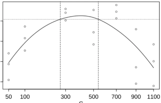
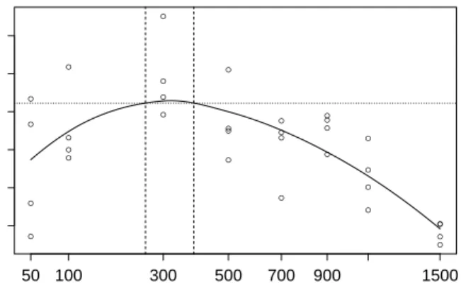
3.1 Estimated profile likelihood forGfrom artificially generated data and the approx-imate 95% confidence interval.. . . 70
3.2 Estimated profile likelihood for G from real case data and the approximate 95% confidence interval. . . 73
3.3 The filter estimates for the SEIR compartment sizes for artificially generated data 76
3.4 Simulated data sequences at various values of Gand the estimated Monte Carlo MLE from real case data . . . 77
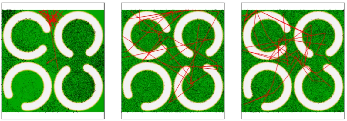
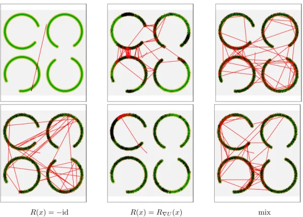
4.1 The first 30,000 sample points from the BPS with varying values ofN for the model with four “C”s . . . 110
4.2 The first 30,000 sample points from the BPS with varying values of N for the inverted four “C” model . . . 111
4.3 The first 30,000 sample points from the BPS with varyingprefand reflection oper-ators for the four “C” model . . . 112
Table
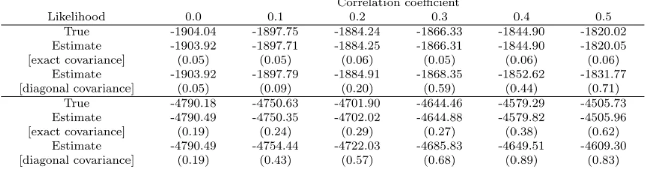
2.1 Log likelihood estimates on a correlated linear Gaussian model with varying di-mensions . . . 40
2.2 Log likelihood estimates on a correlated linar Gaussian model with varying degrees of correlation . . . 40
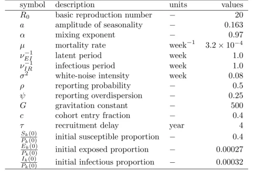
3.1 Model parameters and the values used to generate artificial data . . . 63
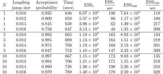
4.1 Acceptance probabilities and effective sample sizes for an ill-conditioned high di-mensional Gaussian model with varying values ofN and leapfrog step size . . . 101
Algorithm
1 A guided intermediate resampling filter (GIRF) . . . 19
2 An iterated guided intermediate resampling filter for parameter estimation . . . 36
3 Multiple proposal Metropolis Hasting algorithm . . . 81
4 Multiple proposal piecewise deterministic MCMC . . . 88
5 Multiple proposal discretized bouncy particle sampler . . . 123
Data analysis can be carried out based on a stochastic model that reflects the analyst’s understanding of how the system in question behaves. The stochastic model describes where in the system randomness is present and how the randomness plays a role in generating data. The likelihood of the data defined by the model summarizes the evidence provided by observations of the system. Drawing inference from the likelihood of the data, however, can be far from being simple or straightforward, especially in modern statistical data analyses. Complex probability models and big data call for new computational methods to translate the likelihood of data into inference results. In this thesis, I present two innovations in computational inference for complex stochastic models.
The first innovation lies in the development of a method that enables inference on coupled dynamic systems that are partially observed. The high dimensionality of the model that defines the joint distribution of the coupled dynamic processes makes computational inference a challenge. I focus on the case where the probability model is not analytically tractable, which makes the computational inference even more challenging. A mechanistic model of a dynamic process that is defined via a simu-lation algorithm can lead to analytically intractable models. I show that algorithms that utilize the Markov structure and the mixing property of stochastic dynamic systems can enable fully likelihood based inference for these high dimensional ana-lytically intractable models. I demonstrate theoretically that these algorithms can substantially reduce the computational cost for inference, and the reduction may be
are inferred from data collected at linked geographic locations, as an illustration that this algorithm can offer an advance in scientific inference.
The second innovation involves a generalization of the framework in which sam-ples from a probability distribution with unnormalized density are drawn using Markov chain Monte Carlo algorithms. The new framework generalizes the widely used Metropolis-Hastings acceptance or rejection strategy. The resulting method is straightforward to implement in a broad range of MCMC algorithms, including the most frequently used ones such as random walk Metropolis, Metropolis adjusted Langevin, Hamiltonian Monte Carlo, or the bouncy particle sampler. Numerical studies show that this new framework enables flexible tuning of parameters and fa-cilitates faster mixing of the Markov chain, especially when the target probability density has complex structure.
Introduction
Inference from the observations of the real world can be made using a stochastic model, which accounts for the randomness in data. The complexity of stochastic models varies with factors such as the complexity of the system in question, the amount of prior knowledge about the system to be incorporated, or the level of flexibility that we require in the model. Given a stochastic model, the information contained in the data is summarized in the likelihood function of the data.
Drawing inference from the likelihood function of the data may not be straight-forward. The more complex the model becomes, the harder it becomes to extract information from this. Unless the likelihood function and the resulting estimators are analytically tractable, the inference will need to rely on computational techniques, through which the aspects of the random system that we are interested in are revealed and understood. Typically the computational tasks involved are the optimization of an objective function, which may be the likelihood function or an approximate ver-sion of it, or sampling from a target distribution, such as the posterior distribution of the parameters. The goal of these tasks is to numerically compute quantities that are useful in drawing inference.
The numerical computational methods may involve either deterministic or
tic operations. The deterministic approach aims to compute certain feature of the target function or distribution using some analytical knowledge about the problem. The stochastic approach constructs artificial random processes that can be used to represent some features of interest of the target statistical object, such as likelihood functions or posterior distributions. The procedure of constructing artificial random processes in a computer is called Monte Carlo simulation. Despite the randomness in the representation, stochastic approaches can be more desirable in certain cases because they can be applied where no deterministic methods are available or can be more computationally efficient than deterministic alternatives.
1.1 Computational challenges
In this thesis, I focus on Monte Carlo approaches to numerical computation of the target statistical quantity. Monte Carlo numerical computation is a vast topic that is studied in diverse fields with different approaches. The methods for Monte Carlo numerical computation are constantly and rapidly evolving to address new challenges imposed by modern data analysis problems. This thesis concerns the following issues that lead to computational challenges.
Analytically intractable likelihood function The likelihood function may not have an analytically tractable form. The likelihood might be expressed as a high di-mensional integral over a number of latent variables, which makes it impossible to evaluate it pointwise with analytical means. Models may also be implicitly defined by data-generating simulation algorithms. These models may not possess analyti-cally tractable densities. Implicit models defined by simulation algorithms can arise frequently when we take a mechanistic approach to set up a stochastic model. Mech-anistic models are based on principled understanding of the system in question, and
the resulting model may only be readily represented via simulation algorithms.
High dimensionality of the model It can be very difficult to computationally rep-resent high dimensional distributions. Monte Carlo approaches to computational inference generate samples from a target distribution, where the empirical distri-bution of the random sample is taken as a stochastic approximation to the target distribution. However, the number of possible states to be represented increases proportionally with the volume of the space, that is, exponentially with the dimen-sionality of the space. The computational cost needed for this representation can also increase exponentially. The steep increase in computational cost is closely tied to the amount of information to be represented.
Complex structure of the target function The target function may have complex structure. The level sets of the target function may have complicated geometric shapes or consist of disjoint connected sets. A target distribution may be constrained in the sense that the probability mass is concentrated in a narrow neighborhood around a lower dimensional hyperplane or manifold. Constrained distributions may arise if the variability in some directions is much smaller than that in other directions, or if random variables constituting the distribution are strongly correlated with each other. Understanding the numerical characteristics of these kinds of target function may require special measures. It can be difficult to find a sampling method that may resolve all difficulties in sampling for various types of complex distributions. In this thesis, I seek to develop a methodological framework with some degree of general applicability that can be useful for a range of sampling problems.
1.2 Overview
In this thesis, I propose two methodological innovations in computational in-ference for complex stochastic models. Relevant background information for each development is provided below, as well as summaries of my contributions.
1.2.1 Inference algorithms for coupled Markov processes with partial observations
Some probability models have certain structure that can be exploited to sub-stantially enhance the efficiency in numerical computations. One instance is where the probability distribution has certain conditional independence structure. Condi-tional independence can be represented by graphical models. A frequently arising conditional independence structure observed in real world examples is the Markov property in temporal contexts. In a Markov process, the past and the future are independent given the present state. Due to this conditional independence structure that is linear in graphical representation, it is often a good strategy to numerically represent the distribution in a sequential manner.
In statistical data analysis framework, Markov process models are often used as a basis on which data are obtained as incomplete or partial observations. The data are modeled to be draws from measurement processes, conditional on the state of the underlying Markov process. The Markov process model and the measurement process model are jointly referred to as a partially observed Markov process (POMP) model. For POMP models, inference often requires understanding the posterior distribution of the Markov process given the data. Unless the model has an analytically tractable form on which the inference procedure can be based, the distribution of the latent Markov process is numerically represented using an ensemble of random draws. The numerical representation of the latent state can be sequentially carried out using
the Markov structure. This approach can reduce the dimension of the space to be computationally represented, because it allows us to deal with the state of the process at a single time point rather than the sequence of states over all time points. Thus, the gain in computational efficiency can be huge compared to approaches that do not take into account the temporal structure.
Sequentially updating the representation of the latent distribution of the Markov process given the observations up to a certain time point is often referred to as a filtering procedure. A filtering procedure can be implemented as sequential impor-tance sampling. At each imporimpor-tance sampling step, additional piece of information provided by the newest observation is incorporated into the computational represen-tation.
Challenges arise when the space is high dimensional, since the number of samples needed to represent a distribution on the space can increase steeply. High dimensional observations can also lead to difficulties, because high dimensional measurement den-sities may designate a small volume in the high dimensional space as the only viable candidates for the hidden state. These difficulties may be manifested by unbalanced weights in importance sampling. Consequently, the numerical representation may become highly variable and lacking in internal diversity.
One approach that aims to solve this issue implements a sequence of bridging distributions. If the proposal distribution in importance sampling is very different from the target distribution in the sense that the ratio between the corresponding densities has high variance, multiple intermediate importance sampling steps that se-quentially target the bridging distributions can reduce the gap between the proposal and the target distribution. Numerically efficient choices for bridging distributions can be obtained with relative ease if both the proposal and the target distribution
have analytically tractable densities.
Contributions I propose an inference algorithm for coupled stochastic dynamic sys-tems with partial observations. I focus on situations where the target distribution is high dimensional and does not have analytically tractable density. As discussed in the previous section, analytically intractable distributions can arise when a mech-anistic model is defined using a simulation algorithm. I show that even for high dimensional analytically intractable distributions, stable importance sampling algo-rithms can be developed that enable inference on coupled Markov processes with partial observations. I demonstrate empirically and theoretically that the proposed algorithm scales more favorably than other methods proposed for high dimensional stochastic process models.
1.2.2 Flexible, numerically efficient sampling from complex distribution using Markov chain Monte Carlo
The task of sampling from a target distribution whose density can be evaluated up to a multiplicative constant arises frequently in Bayesian statistics when the normalizing constant of the posterior distribution is not computable. Markov chain Monte Carlo (MCMC) sampling is a very widely used class of methods for this task. MCMC constructs a Markov chain whose ergodic limit equals the target distribution. There are numerous MCMC methods, and different algorithms exhibit strengths in different circumstances. For example, there are methods known to scale better with increasing dimensions than other methods.
The wide use of MCMC methods is partly due to the fact that there exists a simple methodological strategy that allows for the construction of a Markov kernel that has the target distribution as its stationary distribution. For example, the
Metropolis-Hastings algorithm, which either accepts or rejects a proposal drawn from a kernel with certain probability, constructs a reversible Markov chain with respect to the target distribution.
Contributions I propose a generalization of the Metropolis-Hastings strategy that is conceptually simple and algorithmically easy to implement. This generalization allows for multiple proposals to be made for Metropolis-Hastings type acceptance. The multiple proposal framework can be applied not only to algorithms that use stochastic proposal kernels, but also to algorithms that employ deterministic kernels. The new framework increases flexibility in the implementation of various MCMC algorithms. I show that the enhanced flexibility can lead to increased computational efficiency, especially in tasks of sampling from complex distributions.
1.3 Organization of the thesis
In Chapter 2, I propose a new computational inference algorithm for coupled dynamic processes, which I call a guided intermediate resampling filter (GIRF). I describe the algorithm, provide theoretical results showing that the algorithm scales substantially better than standard methods, and explain how the algorithm can be implemented in practice. I illustrate the favorable scaling to high dimension with numerical results on a toy model. I also explain how parameter estimation can be carried out using this algorithm.
In Chapter 3, I apply the GIRF algorithm for a real scientific inference problem. The spatiotemporal transmission dynamics of measles at linked geographic locations in England and Wales in the twentieth century is analyzed using weekly case reports data. The strength of the spatial coupling of transmission dynamics in various loca-tions is inferred using a fully likelihood based method. This result marks an advance
in inference methodology, because inference on joint properties such as coupling using a fully likelihood based method has been considered difficult and avoided in practice. In Chapter 4, I propose a generalization of the Metropolis-Hastings acceptance or rejection strategy in Markov chain Monte Carlo sampling. I introduce the new framework in a general setting, and explain how this framework can be combined with various MCMC algorithms that are frequently used in practice. Theoretical results showing the validity of the new method are provided, and its relationship with other approaches in the literature is explained. Discussions on how this novel framework can be practically used to improve computational efficiency, including the ways of flexibly tuning parameters in Hamiltonian Monte Carlo algorithms, follow. Numerical results show computational gains of using this framework when sampling from complex distributions.
A guided intermediate resampling particle filter for
inference on high dimensional systems
Sequential Monte Carlo (SMC) methods, also known as particle filter methods, are a basic tool for inference on nonlinear partially observed Markov process (POMP) models. However, the performance of standard SMC algorithms quickly deteriorates as the model dimension increases. We present a novel particle filter which we call a guided intermediate resampling filter (GIRF). The GIRF is readily applicable to a broad range of models thanks to its plug-and-play property of requiring only a simulator of the process but not an evaluator of the transition density for inference. Theoretical and experimental results indicate that the GIRF scales much better than the standard particle filter, suggesting that the GIRF opens new possibilities for inference on highly nonlinear, non-Gaussian dynamic systems of moderate dimension.
2.1 Introduction
Partially observed Markov process (POMP) models offer a framework for likeli-hood based analysis of dynamic systems. A POMP model, otherwise known as the state space model, consists of a Markov state process representing the time evolution of the system and a measurement process that provides partial or noisy information about the states. Sequential Monte Carlo (SMC) methods are recursive algorithms
that enable estimation of the likelihood and the posterior state distributions given data from a POMP model [Doucet et al., 2001, Capp´e et al., 2007, Doucet and Jo-hansen,2011]. These approaches, also known as particle filter methods, approximate state distributions with a collection of simulated random variables, which are called particles.
Inference on some dynamic systems require fitting models with high dimensional state space to high dimensional data. Dynamic processes involving many spatial locations appear in the study of ecological, epidemiological and geophysical systems, for example. For these spatiotemporal models, both the state and measurement dimension tend to scale linearly with the number of spatial locations. Ensemble Kalman filter methods have been used to predict atmospheric dynamics for weather forecasts due to their good scalability to high dimensions [Houtekamer and Mitchell,
2001]. However, these methods can be ineffective for highly nonlinear and non-Gaussian systems, because they rely on locally linear and non-Gaussian approximations [Ades and Van Leeuwen,2015,Lei et al.,2010,Miller et al.,1999]. In systems biology, models for networks of reactions often build upon deterministic differential equations or stochastic simulation [Kitano,2002]. The model dimension typically increases with the number of system components, but even the state-of-the-art inference methods are not suitable for application beyond small systems [Owen et al., 2015].
Particle filter methods suffer from rapid deterioration in performance as the model dimension increases. This phenomenon occurs due to the weight degeneracy among particles. When highly unbalanced weights are given to the particles, resampling results in loss of particle diversity and poor approximation to the state distribution. Theoretical results demonstrating this phenomenon were established by Bengtsson et al. [2008] and Snyder et al. [2008]. These authors found out that the number
of particles required for filtering increases exponentially in the variance of the log density of the observation given the state, which is closely tied to the space dimension. Heuristically, these results indicate that the curse of dimensionality (COD) is related to high dimensional measurement density, implying that particle depletion happens because each observation carries too much information. In this sense, the COD in particle filtering may be understood as a curse of too much information.
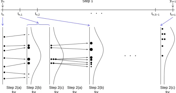
The view that too much information in the observations leads to particle depletion suggests that the difficulty in filtering might be combatted by controlling the rate at which the filtering algorithm introduces new information. We propose such an algorithm, which is shown both in theory and practice to perform well in moderately high dimensions. A high level summary of the algorithm, which we refer to as a guided intermediate resampling filter (GIRF), is as follows.
1. Divide each time interval between observations into sub-intervals, whose number is chosen in accordance with the space dimension of the POMP model.
2. For each sub-interval thus obtained,
(a) Evolve the particles according to the transition kernel of the original state process.
(b) Assess the fitness of each particle to future observations.
(c) Resample the particles with weights reflecting the changes from the previous assessment.
A schematic diagram of this algorithm is provided in Figure 2.1. The assessments at step 2(b) can be made based on the approximations to the predictive likelihoods of a certain number of future observations. This way, the particles with low predictive likelihoods are pruned away, while the particles with higher predictive likelihoods
yn yn+1 tn tn,1 tn,2 tn,S−1 tn+1 ● ● ● Step 1 ● ● ● ● ● ● ● ● ● ● ● ●● ● ● ● ● ● ● ● ● ● ● ● ● ● ● ● ● ● ● ● ● ● ● ● ● ● Step 2(a) for (tn,tn,1) Step 2(b) for (tn,tn,1) Step 2(c) for (tn,tn,1) Step 2(a) for (tn,1,tn,2) Step 2(b) for (tn,1,tn,2) Step 2(c) for (tn,S−1,tn+1)
Figure 2.1: A schematic diagram of a GIRF algorithm
survive and propagate to the subsequent time point. The repeated assessment and resampling steps gradually guide the particles toward the correct posterior state distribution conditional on the data. We will usually set the number of sub-intervals between observations equal to the dimension of the state and measurement space for favorable scaling. This choice is justified in later sections.
In order to simulate the state process over shorter time intervals, we impose a constraint on the model that the transition distribution of the state process is infinitely divisible. Infinite divisibility of the transition distribution is a natural characteristic of all continuous time Markov processes, a widely used class of models across the physical and biological sciences.
We emphasize that a key difference that distinguishes our GIRF from other meth-ods in the literature designed for high dimensional filtering is its practical utility. An inference method that can be implemented with only the simulator of the data gen-erating process is said to have the plug-and-play property [Bret´o et al., 2009, He
et al., 2009]. In the context of SMC, the plug-and-play property means that only a simulator of the state process, but not an evaluator of its transition density, is required for inference. Our GIRF method, possessing the plug-and-play property, facilitates the use of a broad range of models, including mechanistic models defined by simulation algorithms or models defined by stochastic differential equations. Both kinds of models typically have analytically intractable transition densities, but their state processes can be simulated. The sample paths of diffusion processes can be ap-proximately simulated with numerical methods such as the Euler-Maruyama method [Kloeden and Platen,1999]. The plug-and-play property is essential for inference on POMP models whose state processes have intractable transition densities.
Our GIRF algorithm has connections to some well known methods in the particle filtering literature. First, it can be theoretically formulated either as a generaliza-tion or as a special case of the bootstrap filter by Gordon et al. [1993]. The latter interpretation places the algorithm within the general theory of SMC and provides immediate proofs for the unbiasedness of likelihood estimates and other results of convergence for the GIRF. Our method can also be seen as a generalization of the auxiliary particle filter (APF) proposed by Pitt and Shephard [1999]. The APF evolves and weights particles in a way that depends on the next observed data point. This approach often results in improved filtering, although it has been noted that this may not be always the case [Johansen and Doucet,2008]. Our method is similar to the APF in that the particles are guided by oncoming observations. In the GIRF, adapted proposals for the next time step are obtained through a series of propagation and resampling steps at the intermediate time points.
The remainder of the chapter is organized as follows. Section 2.2 reviews several ideas in the literature that are related to high dimensional filtering. Section 2.3
introduces and explains our GIRF method. Section2.4reports some of its theoretical properties, including the main result (Theorem II.2) that establishes a finite sample error bound for the estimates obtained by the GIRF. This result, developed from first principles, offers a novel viewpoint on the filtering error and explains why our GIRF scales better to high dimensions than standard methods. Section 2.5 describes how one can estimate model parameters by combining the GIRF with the iterated filtering scheme of Ionides et al. [2015]. Implementation of our algorithm in Section 2.6
empirically show our algorithm’s favorable scaling and its capability of facilitating spatiotemporal inference that has previously been considered inaccessible due to computational constraints. Section 2.7 concludes with a discussion.
2.2 Previous approaches to high dimensional filtering
Several theoretically motivated algorithms for high dimensional particle filtering have been proposed in the past few years. Rebeschini and Van Handel[2015] consid-ered a filtering method that builds upon the assumption that the interaction between the spatial locations is local. The algorithm partitions the state variables into blocks and approximates the one step transitions of the state process as being independent between the blocks. A theoretical bound for the filtering error was derived, which only depends on the size of the largest block but not on the entire space dimen-sion. Despite this very desirable scaling property, this approach has some practical limitations, because it is not applicable to highly interdependent spatial models and the filter estimates are not reliable near the boundaries of the blocks, which may constitute a substantial fraction of the total number of variables.
Beskos et al.[2014a,b] applied the annealed importance sampling proposed inNeal
annealed importance sampling method introduces a series of bridging distributions between observations, whose densities are set proportional to a fractional power of the desired target density. Between two adjacent importance resampling, the particles are transformed according to a transition kernel whose stationary distribution equals the target bridging distribution. These transition kernels provide mixing that helps maintain the stability of the particle approximations. The authors gave stability results for the case where the original high dimensional state process is composed of many copies of independent and identically distributed (IID) one dimensional processes. In particular, Beskos et al. [2014a] showed that the importance weights are non-degenerate as the dimension goes to infinity even with fixed particle size.
Beskos et al. [2014b] showed that both the L2 error of the filter estimates and the
variance of the likelihood estimates are bounded uniformly in the space dimension. However, the main drawback of this approach, which reduces its practical value, is the absence of the plug-and-play property. Annealed importance sampling requires evaluable analytic expression of the density of the one-step transition in order to build artificial transition kernels between bridging distributions.
Beskos et al. [2017] studied the case where the spatial structure of the model can be hierarchically factorized and investigated the possibility of overcoming the COD. Specifically, they assumed that the one step transition density equals, or can be well approximated by, a product of terms which are functions of the state variables belonging to an increasing sequence of subsets of the dimensions of the space. The theoretical results they obtained by considering a few simple IID cases are promising, because they show that filtering can be stable when the number of particles increases linearly with the space dimension. These results provide useful insights into what might be achieved in more general cases.
Del Moral and Murray [2015] have proposed a particle filtering algorithm for highly informative observations that is almost identical to our method at its core, though our motivation and theoretical analysis differ. The authors were motivated by the study of perfectly observed diffusion processes, which share with high dimen-sional POMPs the difficulty that highly informative observations make computations challenging. In this thesis, I demonstrate the utility of a GIRF in high dimensions, both theoretically and empirically. We show that the GIRF may yield accurate es-timates of the posterior state distributions given the data in high dimensions. In order to further avoid weight degeneracy, our method uses more than one future observations for particle assessment. This potential improvement was less relevant for the precisely measured processes considered by Del Moral and Murray [2015].
2.3 Method
2.3.1 A POMP model and Sequential Monte Carlo
We consider a Markov state process defined in continuous time and denoted by
{Xt;t≥0}, with the random variableXt taking values in a space X. The
measure-ment process yields observations {Yn;n = 1,2, . . . , N} that are incomplete, noisy
measurements of Xt at discrete time points tn >0,n= 1, . . . , N. The measurement
Yn is independent of other observations Ym, m 6=n, and of the state process {Xt},
given the current state Xtn. The observationsYn=yn for n= 1, . . . , N are assumed
to be fixed data. The state process evolves over time according to Markov transition kernels Kt,t0, where 0 ≤ t ≤ t0. That is, the probability distribution of the random
state Xt0 conditioned on Xt =xt is given by
We denote the initial state distribution at time t0 ≥ 0 byµt0. We will occasionally
express the distributions of random variables in terms of their densities. For example, the density of Xtn given Xtm = xtm (m < n) will be denoted by pXtn|Xtm(x|xtm)
with respect to a reference measure on X written as dx. The measurement process forYn conditioned onXtn =xtn is assumed to have density gn(· |xtn). We adopt the
notation n:m ={n, n+ 1, . . . , m}for integersn ≤m. Some quantities of interest in an inference on a POMP model include the likelihood of data
`1:N(y1:N) =E " N Y n=1 gn(yn|Xtn) # ,
where the expectation is taken with respect to the law of {Xt;t ≥ 0}, and the
filtering distribution of Xtn conditioned on the observations y1:n, whose density is
denoted by pXtn|Y1:n(xtn|y1:n).
Particle filter methods operate by recursively approximating the filtering distribu-tions. The approximation at time tn is realized by the sample draws{X
j
tn;j ∈1 :J}
and associated importance weights {w˜j;j ∈1 :J}. The weighted sum of point mea-sures (2.1) J X j=1 ˜ wjδXj tn(dx)
is taken as an approximation to the filtering distribution. Heading to the next time point tn+1, the particle filter first draws samples from the discrete weighted
distribution (2.1). This step is called resampling. Next in the propagation step, the resampled particles are independently transformed according to some transition kernel. A set of importance weights are given to the transformed particles, such that the new weighted sum represents the filtering distribution of Xtn+1 conditioned on
y1:n+1. The choice of the propagation kernel affects the performance of the particle
determines the stability of the resulting estimates.
2.3.2 Guided intermediate resampling filter
In what follows, we assume that the transition kernel of the state process can be simulated but do not require its density to be evaluated. We also assume that the state transition kernels Kt,t0 for the state process {Xt;t ≥0} are infinitely divisible
and can be expressed as
Kt,t0 =Kt,τ1Kτ1,τ2· · ·Kτ
n−1,τnKτn,t0
for any number of intermediate time points t ≤τ1 ≤ · · · ≤τn ≤t0. For
implementa-tion of our GIRF algorithm, we pick S−1 intermediate time pointstn,s,s ∈1 :S−1,
within the observation time interval [tn, tn+1] such that
tn,0 :=tn < tn,1 <· · ·< tn,S−1 < tn,S :=tn+1
for n ∈ 0 :N−1. As a rule of thumb, we will take S = d, the dimension of the measurement space.
The algorithm starts with an initial swarm ofJ particles{Xt0F,j;j ∈1 :J}of equal weights that represent the initial distribution of Xt0. The superscript F stands for
“filtered particles”. The algorithm proceeds recursively. Suppose at some timetn,s−1,
we have a collection of particles, denoted by {XtF,jn,s−1;j ∈ 1 :J}. The particles are transformed according to the transition kernel Ktn,s−1,tn,s and called the proposed
particles, denoted by {XtP,jn,s;j ∈ 1 :J}. These proposed particles at time tn,s are
assessed based on how likely they are to generate the future observations yn+1:n+B
for some B ≥ 1. The assessments are made by what we call the guide function, utn,s: X→ R
+. At the initial time point we require that u
t0(x) ≡ 1 and at the last
Algorithm 1: A guided intermediate resampling filter (GIRF) Input :Simulator for µt0(dx)
Simulator for Ktn,s−1,tn,s(dx;xtn,s) forn∈0 :N−1 ands∈1 :S
Evaluator forgn(yn|xtn) forn∈1 :N
Evaluator forutn,s(xtn,s) forn∈0 :N−1 ands∈1 :S
Data,y1:N
Number of particles,J
Output:Filtered particle swarm, nXtF,j
N ;j∈1 :J o Likelihood estimate, ˆ` Initialize: `ˆ←1,XtF,j 0 ∼µt0(dx) forj∈1 :J, andu j old←1 for j∈1 :J forn←0 :N−1do If n≥1thenujold← u j old gn yn X F,j tn forj∈1 :J fors←1 :S do XtP,jn,s ∼Ktn,s−1,tn,s dx;XtF,jn,s−1forj∈1 :J uj new←utn,s XtP,j n,s forj∈1 :J wj←ujnew/u j old forj∈1 :J ˆ `←`ˆ×PJj=1wjJ Drawaj withP aj=i=wiPJi0=1wi 0 forj∈1 :J
SetXtF,jn,s =XtP,an,sj andujold=uaj
new forj∈1 :J
end
SetXtF,jn+1,0 =XtF,jn,S forj ∈1 :J
end
tn,s, s∈ 1 : S, is determined by the ratio of the assessments at time tn,s and tn,s−1.
The algorithm sets the weight for the j-th particle to be (2.2) wj =wtn,s XtP,jn,s, XtF,jn,s−1:= utn,s XtP,jn,s utn,s−1 XtF,jn,s−1 if tn,s−1 ∈/ t1:N utn,s XtP,jn,s utn,s−1 XtF,jn,s−1 . gn yn X F,j tn,s−1 if tn,s−1 ∈t1:N.
If tn,s−1 ∈ t1:N, the denominator is divided by gn yn
xFt
n
, because at time tn,s =
tn,1 > tn, the past observation yn should no longer be considered in assessing the
fitness. The weights at observation times tn are taken as wtn−1,S(X
P,j
tn−1,S, X
F,j
tn−1,S−1).
The particles are then resampled with normalized weightswj/PJ
as {XtF,jn,s;j ∈ 1 :J}. The pseudocode for our method is shown in Algorithm1. Our
implementation of the GIRF is available at https://github.com/joonhap/GIRF.
git.
The likelihood estimate ˆ` of `1:N(y1:N) is obtained from Algorithm 1. This
quan-tity can be much more stable than the likelihood estimate obtained from the stan-dard bootstrap particle filter in high dimensions. This claim is supported by The-orem II.2 and by the argument given in the appendix section 2.B. Algorithm 1
is equivalent to the bootstrap particle filter if we take S = 1 and utn(xtn) =
gn(yn|xtn). It is equivalent to the auxiliary particle filter if we take S = 1 and
utn(xtn) = gn(yn|xtn)·gn+1 yn+1|µtn+1(xtn)
where µtn+1(xtn) denotes a
determin-istic or stochastic prediction for the state at time tn+1 based on Xtn =xtn.
The particle swarm {XtF,jn,s;j ∈1 :J} at timetn,s targets a density proportional to
(2.3) utn,s xtn,s ·pXtn,s|Y1 :n xtn,s y1 :n .
When utn,s(xtn,s) approximates pYn+1:n+B|Xtn,s(yn+1:n+B|xtn,s), the above expression
(2.3) approximates the conditional density pXtn,s|Y1:n+B(xtn,s|y1:n+B).
The following simple argument shows that (2.2) makes Algorithm 1 a properly weighted filter [Liu,2008, Definition 2.5.1]. For each particleXtF,jn,s, we define a parent particle at time tn,s−1 as follows: if XP,a
j
tn,s for some a
j ∈ 1 :J was called XF,j tn,s after
resampling, then XtF,an,sj−1, which propagated to XtP,an,sj, is the parent particle of XtF,jn,s. By successively tracing the parent particles, one can construct the ancestral lineage of a particle. Take a particle XtF,jN at time tN and call its ancestor at time tn,s as
XF,a
j tn,s
tn,s , where we write a
j
tN = j. It turns out that the product of all importance
density of y1:N given the states X F,ajtn tn : (2.4) N−1 Y n=0 S Y s=1 wtn,s XP,a j tn,s−1 tn,s , X F,ajtn,s− 1 tn,s−1 = "N−1 Y n=1 gn yn XF,a j tn tn # · N−1 Y n=0 S Y s=1 utn,s XF,a j tn,s tn,s utn,s−1 XF,a j tn,s−1 tn,s−1 = "N−1 Y n=1 gn yn XF,a j tn tn # · utN XF,a j tN tN ut0 XF,a j t0 t0 = N Y n=1 gn yn XF,a j tn tn .
The computational cost of Algorithm 1 typically scales as O(J Sd). If we take S =d and use a fixed number of particles, it scales as O(d2). However, the number of particles will generally need to increase with d in order to keep the errors at a constant order of magnitude. In Section 2.4, we show a novel theoretical result on the filter accuracy, namely that for any f with kfk∞ ≤1,
1 J J X j=1 f XtF,jN −Ef(XtN)|Y1:N =y1:N ≤v(S)
with high probability, where the boundv(S) depends on the number of sub-intervals per observationS, the space dimensiond, the number of particlesJ, the choice of the guide functions utn,s, and other attributes of the POMP model. The rate at which
the number of particles is required to increase withdcan be deduced from the bound v(S).
2.3.3 Choice of the guide functions
Although Algorithm 1 is a properly weighted filter for any guide function utn,s :
X → R+, its numerical efficiency depends on the choice of the guide function. We
take utn,s(x) to be an approximation to the predictive likelihood of yn+1:n+B given
Xtn,s =x,
Whenn+B > N, we takeutn,s(x)≈pYn+1:N|Xtn,s(yn+1:N|x) instead. At observation
times tn, n ∈ 1 :N, the guide function utn is defined as utn−1,S. We illustrate how
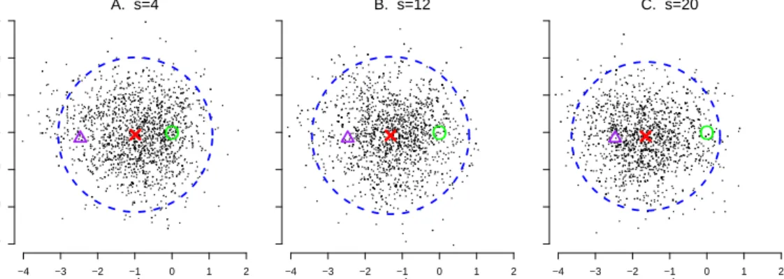
the algorithm works with this guide function using a simple example consisting of a twenty dimensional Brownian motion and a measurement process independent in each dimension. The POMP model is defined on the interval [t0, t1] as
(2.6) Xt0 ∼N(0, I), Xt0 Xt∼N Xt, t0−t t1−t0 I for t ≤t0, Yt1 Xt1 ∼N(Xt1, I).
Here,Idenotes the twenty dimensional identity matrix. The guide function was set to be the exact predictive likelihood withB = 1, namelyut0,s(x) := pY1|Xt0,s(y1|x). The
time interval [t0, t1] was divided intoS= 20 sub-intervals of equal length. Figure2.2
shows the first two coordinates of the filtered particles Xt0F,j,s at three intermediate time points. The mean of the initial distribution is marked by a green ‘O’, and the observation y1 by a purple triangle. At time t0,s, the conditional distribution given
Y1 =y1 equals Xt0,s (Y1 =y1)∼N 1 3 1 + s S y1, 13 1 + Ss 2− s S I . The mean of this conditional distribution for eachs is marked by a red ‘X’, and the 95% coverage region by a blue dashed circle. As time progresses, the red ‘X’ shifts from the origin toward y1, and the coverage region changes in size. The filtered particles almost
exactly follow the conditional distributions at the intermediate steps, showing that they are gradually guided toward pXt1|Y1 as s increases from zero to twenty.
If the guide function is taken as in (2.5) andSis close to the space dimensiond, the GIRF may be rescued from the weight degeneracy. We now give a heuristic argument for this claim. TheoremII.2in Section2.4will provide a rigorous argument. First, we consider the resampling weights for s≥2. Suppose the ancestors of a particleXtF,jn+1 are denoted by XF,a
j tn,s
tn,s ;s ∈ 1 :S , where a
j
−4 −3 −2 −1 0 1 2 x 2 −3 −2 −1 0 1 2 3 x1 A. s=4 O −4 −3 −2 −1 0 1 2 x1 B. s=12 O −4 −3 −2 −1 0 1 2 x1 C. s=20 O
Figure 2.2: The first two coordinates of the filtered particlesXtF,j0,s from a GIRF run at three inter-mediate time steps (A,s=4 ; B,s=12; C,s=20) for twenty dimensional linear Gaussian model given by (2.6). weights wtn,s X P,ajtn,s −1 tn,s , X F,ajtn,s −1 tn,s−1 fors ∈2 :S approximates S Y s=2 wtn,s XP,a j tn,s−1 tn,s , X F,ajtn,s −1 tn,s−1 = utn+1 XtF,jn+1 utn,1 XF,a j tn,1 tn,1 ≈ pYn+1:n+B|Xtn+1 yn+1:n+B X F,j tn+1 pYn+1:n+B|Xtn,1 yn+1:n+B XF,a j tn,1 tn,1 .
The logarithm of the right hand side of the above expression can be expected to be of orderOp(Bd) if the POMP model consists ofdweakly coupled processes, for which
behavior should be similar to the IID case. Thus, if the termswtn,s X
P,ajtn,s− 1 tn,s , X F,ajtn,s− 1 tn,s−1
for s ∈ 2 :S are of roughly the same magnitude, the logarithm of each resampling weight may be on the order of S−11Op(Bd). If we take S = d and B is not too
large, the resampling weights may be Op(1) in d. This reasoning is closely related to
Assumption 2 in Section 2.4.
The resampling weights at s=1 require additional consideration. The resampling weight for XtP,jn,1 is given by
(2.7) utn,1 XtP,jn,1 utn XtF,jn .gn yn X F,j tn ≈ pYn+1:n+B|Xtn,1 yn+1:n+B X P,j tn,1 pYn:n+B−1|Xtn yn:n+B−1 X F,j tn . gn yn X F,j tn = pYn+1:n+B−1|Xtn,1 yn+1:n+B−1 X P,j tn,1 pYn+1:n+B−1|Xtn yn+1:n+B−1 X F,j tn ·pYn+B|Xtn,1,Yn+1:n+B−1 yn+B X P,j tn,1, yn+1:n+B−1 .
The term pYn+1:n+B−1|Xtn,1 yn+1:n+B−1|X P,j tn,1 pYn +1:n+B−1|Xtn yn+1:n+B−1|X F,j tn
may be of Op(1) by the same reasoning
as above. The term pYn+B|Xtn,1,Yn+1:n+B−1(yn+B|X P,j
tn,1, yn+1:n+B−1) is related to the
mixing of the POMP conditional on data. Conditional mixing of a POMP means that a distant future observation provides substantially less information about the current state than the nearest future observation does, provided that all the obser-vations until that distant time point are already known. The additional information about Xtn,s provided by yn+B when yn+1:n+B−1 are known is represented by the
like-lihoodpYn+B|Xtn,s,Yn+1:n+B−1 yn+B
xtn,s, yn+1:n+B−1
.Under conditional mixing, this likelihood yields balanced values when evaluated at the support of the distribution pXtn,s|Y1:n+B−1(xtn,s|y1:n+B−1). Since an approximation to this distribution is targeted
by the particles{XtP,jn,1;j ∈1 :J}, the values ofpYn+B|Xtn,1,Yn+1:n+B−1(yn+B|X P,j
tn,1, yn+1:n+B−1)
for j ∈ 1 :J may be balanced. Thus, the resampling weight at s=1 shown in (2.7) may not suffer from weight degeneracy, if conditional mixing is obtained for B not too large. Assumption 3 in Section 2.4 formalizes the conditional mixing argument in a manner that is relevant to our theoretical investigation.
The state distribution conditioned on several future observations is called the fixed lag smoothing distribution. Its use for stable filtering has been studied in the litera-ture, for example, in Clapp and Godsill[1999], Chen et al.[2000], and Doucet et al.
[2006]. Our contribution is to connect this approach with intermediate resampling algorithms and the COD. Fixed lag smoothing distributions tend to be less affected by outliers in the observed data than filtering distributions [Lin et al., 2013]. Intu-itively, looking ahead to B observations in the future for particle assessment allows the information provided by the observationyn+B to be processed over a longer time
Practical design of the guide functions
In practical situations, finding a good approximation to the predictive likelihood of future observations can be a difficult task. It may be particularly demanding when the transition density of the state process is intractable, which is the situation when plug-and-play methods are particularly desired. Therefore, designing practically ac-cessible guide functions is critical in the application of the GIRF. Here we suggest several ways of making such designs.
1. Semi-analytical approach with moment matching The predictive likelihood of multiple future observations is typically more difficult to estimate than the predictive likelihood of a single observation. Thus after approximating pYn+b|Xtn,s yn+b
xtn,s
and calling the approximation utn,s%tn+b for b∈1 :B, we may set
(2.8) utn,s xtn,s = B Y b=1 utn,s%tn+b xtn,s .
Fors =S and b= 1, we can evaluate the measurement density attn,S =tn+1, so we
set utn,S%tn+1 xtn,S =gn+1 yn+1 xtn,S .
The approximate predictive likelihood utn,s%tn+b may be taken sensibly depending
on the model. We suggest one way as follows. First, we make a projection from the current state Xtn,s = xtn,s to time tn+b with a deterministic process that
ap-proximates the conditional mean of the state process {Xt;t≥tn,s} given xtn,s. The
projected state will be denoted by ˜xtn+b. We also assume that the variability of
Xtn+b given Xtn,s = xtn,s according to the law of the state process can be
approxi-mately characterized by Σ1(xtn,s). We assume that the measurement density of Yn+b
Σ2(˜xtn+b). We make the dependence explicit by writing gn+b
· |x˜tn+b, Σ2(˜xtn+b)
. The combined variability, denoted by Σ1 xtn,s
+ Σ2 x˜tn+b
, is then taken as the scale parameter for the approximate predictive likelihood of Yn+b given the current
state Xtn,s =xtn,s. In other words, we define
(2.9) utn,s%tn+b xtn,s :=gn+b yn+b x˜tn+b,Σ1 xtn,s + Σ2 x˜tn+b .
If the state process distribution and the measurement distribution belong to dif-ferent scale families, utn,s%tn+b may be obtained by approximating an unnormalized
convolution density (see Section3.2 for an example).
2. SMC-type likelihood estimation for models with weakly interacting state variables
For certain POMP models, the correlation between the components of the state process {Xt} may be weak. For example, the state process may be a collection of
coupled dynamic processes corresponding to different geographic locations, where the dynamics at one location is affected by the dynamics at other locations only by a small degree. When the correlations between the components of {Xt} are weak,
we may use the following approximation:
(2.10) pY n+1:n+B|Xtn,sj (y [1:d] n+1:n+B|X j tn,s)≈ d Y i=1 pY[i] n+1:n+B|Xtn,s (y[ni+1:] n+B|Xtjn,s). Here, the superscripts between brackets indicate the component of the observa-tion variable: yn[1:+1:d]n+B denotes the original d-dimensional observation vectors, and y[ni+1:] n+Bdenotes thei-th components of the observation vectors. The approximation (2.10) can be particularly valid and useful in the cases where each observationy[ni]
de-pends only onXt[in], which is not uncommon, and where the measurement distribution has large variance relative to the variability of the state process. This approximation may be understood in connection with variational inference.
Each term in the right hand side of (2.10) can be estimated using a standard SMC algorithm, where only the observations yn[i+1:] n+B are used in filtering. The procedure is described as follows. For each particle Xtjn,s at time t in the GIRF algorithm, we use J0 number of particles, all of which is initialized atXtjn,s. The joint state process
{Xt}is used to simulate the particle forward in time. The standard bootstrap SMC
algorithm is run for the time period from time t to tn+B. The J0 particles in each
time step (saytn+b) are weighted according to the measurement density of onlyyn[i+]b.
Since the measurement density is one dimensional, the weights will be as balanced as in one dimensional filtering problems. Thus pY[i]
n+1:n+B|Xtn,s
(yn[i+1:] n+B|Xtjn,s) may be precisely estimated using only a moderate number of particles J0, and there will be no need to go through intermediate time steps as in the GIRF algorithm. Note that this procedure still takes into account the coupling between the components of
{Xt}, because we use the joint state process {Xt} for particle propagation; only the
observations for other components are ignored for filtering.
The computation of the likelihood estimates ˆp(yn[i+1:] n+B|Xtjn,s) may seem costly. The computation for each particle Xtjn,s scales as O(J0d2). The total computational cost of running the GIRF thus scales asO(J N SJ0d2). When we takeS =d, the cost scales as the cube of the space dimension. However, this seemingly steep cost is much more favorable than the typical exponential increase for standard SMC methods. For weakly coupled POMP models, this method may enable analyses that are otherwise infeasible.
A potential issue in the approximation (2.10) is that the likelihood estimate ˆ
p(yn[i+1:] n+B|Xtjn,s) has Monte Carlo variability. The resampling weights in the main GIRF are given by the ratio of these likelihood estimates between two consec-utive intermediate time points. The ratio can be unstable if the variability in
ˆ
p(yn[i+1:] n+B|Xtjn,s) is high. A moderately large number of J0 will often be able to make the variance in the likelihood estimates sufficiently small. However, a seed fixing strategy may additionally help in stabilizing the ratio between the likelihood estimates. For the estimation of ˆp(yn[i+1:] n+B|Xtjn,s), the same seed may be used for every j ∈ 1 :J at every intermediate time point tn,s. Then, since the computation
of ˆp(y[ni+1:] n+B|Xtjn,s) and ˆp(yn[i+1:] n+B|Xtjn,s+1) use the same sequence of random num-bers, the Monte Carlo variability in both computations will likely cancel each other, making the ratio less variable. Of course, the fixed random seed should be used only for the likelihood estimation, and the random numbers used for all other operations (i.e., those used in the main GIRF algorithm) should not be affected.
3. Artificially increased variances of measurement densities In estimatingpYn+1:n+B|Xtn,s,
artificially increasing the variances of the measurement densities can help make the likelihood estimates more stable. When pYn+1:n+B|Xtn,s is estimated using the SMC
type approach described above, artificially increased measurement densities can make the estimates ofpYn+1:n+B|Xtn,s have less Monte Carlo variability. Svensson et al.[2018]
have recently shown empirical results illustrating the advantages of using artificially increased variance of measurement densities. When using analytical methods for approximating the likelihood, larger measurement variances can yield more balanced values of approximated likelihood estimates among particles. Even when the ap-proximation of the likelihood is inaccurate, balanced estimates can reduce numerical problems in resampling of particles in the GIRF algorithm.
2.4 Theoretical results
We first introduce some notation. For a bounded measurable function f ∈ Bb(X),
respect to a Markov kernel K conditional on the starting state x by Kf(x). The propagation of measure µ by a kernel K is defined as (µK)f := µ(Kf). At the time step tn,s in Algorithm 1, we denote the empirical distributions corresponding
to the proposed particles and the filtered particles by FtPn,s,J = J1 PJ
j=1δXtn,sP,j and
FtFn,s,J = 1JPJ
j=1δXtn,sF,j respectively. The empirical distribution of the J matching
pairs XtP,jn,s, XtF,jn,s−1 on the product space X2 will be denoted by Htn,s,J. The σ
-algebra generated by the set of random draws DtPn,s := {XtF,j
n0,s0;tn0,s0 ≤ tn,s−1, j ∈
1 :J} ∪ {XtP,j
n0,s0 ;tn0,s0 ≤tn,s, j ∈1 :J} is denoted by B
P
tn,s,J, and the σ-algebra
gener-ated byDtPn,s∪ {XtF,jn,s;j ∈1 :J} is denoted byBF
tn,s,J.
Our GIRF can be cast into the framework of the standard particle filters by extending the state space toX2where the new state variable is the pair (Xtn,s−1, Xtn,s).
This extension is necessary because the resampling weights (2.2) depends on both XtP,jn,s andXtF,jn,s−1. The likelihood estimates obtained from the standard particle filters are unbiased [Del Moral and Jacod, 2001]. It follows that the likelihood estimates from the GIRF are also unbiased. The consistency and the asymptotic normality of the filter estimates from the GIRF also follow naturally from the standard particle filter theory [Chopin,2004, Del Moral, 2004].
Theorem II.1. The likelihood estimate `ˆof Algorithm 1 is unbiased for `1:N(y1:N).
Proof. See Section2.A.
Next we show that the particle approximation to the filtering distribution by Algorithm 1 can have significantly smaller error than the standard filters in high dimensions. The GIRF converts a filtering problem with highly informative observa-tions into one that deals with a slower rate of incoming information at the expense of operating on a refined time scale. Thus mixing of processes happens over greater
number of time steps in this stretched time scale. For this reason, results in the literature which imply that the number of particles needs to increase exponentially in the number of time steps needed for conditional mixing, such as Theorem 3.1 of Del Moral and Guionnet [2001], is not very useful in this case. When we take S = d, a bound increasing exponentially in S is no better than a bound increasing exponentially in d. A new type of error bound will be given below that increases linearly in the number of time steps.
We introduce some more notation. For any t, t0 such that t0 ≤ t ≤ t0 ≤ tN, we
define (2.11) Qt,t0(f)(Xt) :=E f(Xt0) Y t≤tn<t0 gn(yn|Xtn) Xt ,
for any bounded measurable function f. Note that, if no observation was made in [t, t0), we have
(2.12) Qt,t0(f) = Kt,t0f,
and if a single observation tn was made in this interval,
(2.13) Qt,t0(f) = Kt,t
n{(Ktn,t0f)·gn(yn| ·)}.
The collection {Qt,t0;t ≤t0} forms a semigroup, in the sense that Qt,τQτ,t0(f) =
Qt,t0(f) for t≤ τ ≤ t0 [Del Moral,2004]. We denote the set of all intermediate time
points in Algorithm 1 by T = {tn,s;n ∈ 0 :N−1, s ∈ 1 :S}. Given that one has
filtered particles {XtF,j;j ∈1 :J} at time t∈T, we define for t0 ∈T∩[t, tN]
(2.14) bt,t0(f) :=
Z Q
t,t0(ut0 ·f)
ut
dFt,JF
for all bounded measurable functions f on X. Note that this definition implies bt,t(f) =
R
f dFF
t− =tn,s−1. If t= tm for some m ∈ 0 :N, we will write n(t) = m. Since resampling
weights at time t are proportional to wt(XtP,j, X F,j t− ), we have (2.15) E Z f(xt)dFt,JF (xt) Bt,JP = Z f(xt)·wt(xt, xt−)dHt,J(xt, xt−) Z wt(xt, xt−)dHt,J(xt, xt−) .
The conditional expectation of the numerator in the above expression with respect to BF t−,J equals E Z f(xt)·wt(xt, xt−)dHt,J(xt, xt−) BF t−,J = Z K t−,t(ut·f) ut− dFtF−,J if t−∈/ t1:N Z K t−,t(ut·f) ut− ·gn(t−)dFtF−,J if t−∈t1:N = Z Q t−,t(ut·f) ut− dFtF−,J =bt−,t(f), (2.16)
by (2.2), (2.12), (2.13), and (2.14). Note that here we implicitly assumed that gn(t−)
is a function of Xt−, such that gn(t−)(Xt−) := gn(t−)(yn(t−)|Xt−). At time tN, we are
interested in knowing how accurate the quantitybtN,tN(f) =
1 J PJ j=1f(X F,j tN ) is as an
approximation to E[f(XtN)|Y1:N = y1:N]. We establish a bound on the error in this
approximation under a set of assumptions.
Our first assumption concerns how close the guide function ut is to the predictive
likelihood of B future observations. In what follows, if t = tm,s for some s ∈ 1 :S,
we will write t→ := t(m+B)∧N, where we write a∧b = min(a, b). The expression
Qt,t→(gn(t→))(x) denotes the predictive likelihood of Ym+1:n(t→) = ym+1:n(t→) given
Xt=x, see (2.11).
Assumption 1. There exists a constant C1 ≥1 such that for all t ∈T,
(2.17) Qt,t → gn(t→) ut (x)≤C1 Qt,t→ gn(t→) ut (x0),
for all x, x0 ∈X. In particular, if t∈(tN−B, tN]∩T, Qt,tN(gN) ut (x)≤C1 Qt,tN(gN) ut (x0), for all x, x0 ∈X.
Uniform bounds across Xas in (2.17) typically follows as a result of the compact-ness of the spaceX and the continuity of the functions being bounded. However, we do not expect that the compactness condition is critical in real applications of the algorithm.
Our second assumption says that the predictive likelihood of future observations experiences a bounded change between two consecutive intermediate points t− and t. Specifically, we assume that conditioned on Xt−, the predictive likelihood given
Xt has bounded variance relative to the square of its mean.
Assumption 2. There exists C2 ≥1 such that for all t∈T and for all x∈X, Kt−,tQt,t→ gn(t→) 2 Kt−,tQt,t→ gn(t→) 2 (x)≤C 2 2.
Assumption 2 is related to a key reason that a GIRF operates on a refined time scale. If the time interval was not divided, the constant C2 would typically
in-crease exponentially as the space dimension d increases. To see this, if we consider a POMP consisting of d IID one-dimensional processes, the predictive likelihood Qt,t→(gn(t→))(Xt) will be expressed as a product ofd independent random variables.
Thus both its mean and variance will be exponential in d. In a GIRF, however, the constant C2 can be of constant order in d, if we divide the time interval into d
sub-intervals. Examples are given in the online supplementary text 2.D to illustrate this point.
We lastly assume that the POMP has a reasonable amount of conditional mix-ing. We note that, when tm < t ≤ tm+1, the likelihood of Ym+B+1:N = ym+B+1:N
conditioned on Ym+1:m+B =ym+1:m+B and the current state Xt is given by pYm+B+1:N|Xt,Ym+1:m+B (ym+B+1:N|x, ym+1:m+B) = pYm+1:N|Xt(ym+1:N|x) pYm+1:m+B|Xt(ym+1:m+B|x) = Qt,tN(gN) Qt,t→ gn(t→) (x).
Also, for any bounded measurable function f on Xwe have
E[f(XtN)|Xt=x, Ym+1:N =ym+1:N] =
Qt,tN(gN ·f)
Qt,tN(gN)
(x).
Assumption 3. There exist constants C3 ≥1 such that for all t∈T,
(2.18) Qt,tN(gN) Qt,t→ gn(t→) (x)≤C3 Qt,tN(gN) Qt,t→ gn(t→) (x0)
for all x, x0 ∈ X. Also, there exists n∗ ∈ 1 :N−1 and C4 ∈ (0,1) such that for any
measurable function f with kfk∞≤1,
(2.19) Qtn∗,tN(gN ·f) Qtn∗,tN(gN) (x)− Qtn∗,tN(gN ·f) Qtn∗,tN(gN) (x0) ≤C4 for all x, x0 ∈X.
The first inequality (2.18) states that, conditioned on the observationsym+1:(m+B)∧N,
the probability of having the later observations y(m+B+1)∧N:N has bounded
depen-dence on the current state Xt. One can makeC3 smaller by takingB larger, because
more conditional mixing will happen in the longer interval [t, tm+B+1]. The second
inequality (2.19) says that the state at time tn∗ has bounded influence on the state
at tN, conditional on the observations made after time tn∗. One can similarly make
C4 smaller by taking n∗ more distant from N.
We also assume that multinomial resampling is used in Algorithm 1. The indices aj are drawn independently of each other given {wj;j ∈1 :J} under multinomial resampling.