An Efficient Load Balancing Algorithm for P2P Systems

An Efficient Load Balancing Algorithm for P2P

Systems

Khaled Ragab

Computer Science Dept., College of Computer Science and Information Technology, Hofuf, Saudi Arabia

[email protected]

Abstract—Peer-to-Peer (P2P) networks are considered to be the most important development for content distribution and sharing infrastructures. The quality of services provided by the majority of the P2P systems is questioned. Load balancing among peers is critical and a key challenge. This paper proposes a load balancing algorithm based on stochastic analysis. It addresses the out-of-date problem as a result of node’s state changes during loads movement among nodes.

Index Terms— Peer-to-Peer, Overlay Networks, load balancing.

I. INTRODUCTION

In recent years the development of distributed systems especially the internet has been influenced heavily by the

Peer-to-Peer (P2P) paradigm. P2P is a class of

applications that takes advantage of resources e.g., storage, cycles, content, human presence, available at the edges of the Internet [1]. P2P systems offer an alternative to such traditional client-server systems for several application domains. They have emerged as an interesting solution for content distribution, sharing and locating resources over the Internet. In P2P systems, every node (peer) of the system acts as both client and server (servant) and provides part of the overall

resources/information available from the system. Each node often has different resource capabilities (e.g. processor, storage, and bandwidth) [2]. Thus, it is required that each node has a load proportional to its resources capabilities. On account of the dynamism natures of the P2P systems, it is difficult to ensure that the load is uniformly distributed across the system. In particular, this paper considers a P2P system of M nodes in which nodes join/leave, and data entity inserted/deleted continuously. Similarly to [3], [4], [5] this paper assumes node and data entity have been assigned identifiers that chosen randomly. Thus, there is a Θ(log M) imbalance factor in the number of data entities stored at a node. Additionally, the imbalance factor becomes more worse if the P2P applications associate semantics with data entity IDs since IDs will

not be uniformly distributed. Consequently, it is important to design mechanisms that balance the system load. There are two distinct strategies to distribute the system workload [6]. First, load balancing algorithms that strive to equalize the workload among nodes. Second, load sharing algorithms which simply attempt to assure that no node is idle while jobs at other nodes are waiting for service.

Load balancing techniques in P2P systems should be scalable and cope with its large size. They should place or re-place shared data entities optimally among nodes while maintaining an efficient overlay routing tables to redirect queries to the right node.

The communication delays among peers significantly alter the expected performance of the load balancing schemes. Due to such delay, the information that a particular peer has about other peers at any time is dated and may not accurately represent the current state of the other peers. For the same reason, a load sent to a recipient peer arrives at a delayed instant. In the mean time, however, the load state of the recipient peer may have considerably changed from what was known to the transmitting peer at the time of load transfer. This paper proposes a stochastic dynamic load balancing algorithm that tackles the out-of-date problem.

The remainder of this paper is organized as follows. Section two introduces a survey for the load balancing algorithms. Section three exposes the proposed stochastic load balancing model and algorithm. Evaluation of the proposed has been discussed in section four. Section five draws a conclusion of this paper.

II.LOAD BALANCING SURVEY

Load balancing is the problem of mapping and remapping workload in the distributed system.

A. Load Balancing Design

Load balancing design determines how nodes communicate and migrate loads for the purpose of load balancing. It moves workload from heavily loaded nodes (senders) to lightly loaded nodes (receivers) to improve the system overall performance [15]. Load balancing design includes four components that can be classified as follows [16] [17].

• Transfer policy: It decides whether a node is in a suitable state to participate in a load transfer; either Manuscript received February 15, 2011; revised May 15, 2011;

accepted July 15, 2011.

The author is on leave holiday from Ain Shams University, Cairo, Egypt.

receiver or sender.

• Location policy: Once the transfer policy decides that a node is a receiver or sender. The location policy takes the responsibility to find a suitable sender or receiver.

• Selection policy: Once the transfer policy decides that a node is a sender, the selection policy specifies which load should be transferred. It should take into account several factors such as load transfer cost, and life time of the process that should be larger than load transfer time.

• Information policy: It decides when and how to collect system state information.

Load balancing designs are categorized into static and dynamic. With a static load balancing scheme, loads are scattered from sender to receiver through deterministic splits. Static schemes are simple to implement and easy to achieve with slight overhead [13]. They perform perfectly in homogenous systems, where all nodes are almost the same, and all loads are same as well. On the other hand, the dynamic load balancing schemes make decisions based on the current status information [15]. Accordingly, the transfer policy at certain node decides to be a sender or receiver, the selection policy selects the load to be transferred. The dynamic load balancing schemes perform efficiently when its nodes have heterogeneous loads, and resources. The typical architectures of dynamic load balancing schemes can be classified into centralized, distributed, and topological. In a centralized scheme, a central server “coordinator” receives load report from the other nodes, while overloaded nodes request the coordinator to find underloaded nodes [17]. In distributed architecture, each node has a global or partial view of the system status. Consequently, the transfer policy at each node can locally decide to transfer a load either out from it (sender-initiated) or into it (receiver-initiated) [18]. Then, the location policy at each node probes a limited number of nodes to find a suitable receiver or sender. P. Kruger [19], proposed symmetrically-initiated adaptive location policy that uses information gathered during its previous searches in order to keep track of the recent state of each node in the system. It finds a suitable receiver when a heavily-loaded node wishes to send a load out, and finds a suitable sender when a lightly-loaded node wishes to receive a load. Finally, in a system with large number of nodes, a topological scheme should be used [20]. It partitions nodes into groups. The load balance is performed in each group first, then, a global load balance among groups will be performed. However nodes in the hierarchical architecture [21] are organized into a tree. Inner nodes gather the status information of its sub-trees. Then, load balancing is performed the leaves to the roots of the tree. B. P2P Load Balancing

Load balancing is a critical issue for the efficient operation of the P2P systems. Recently, it attracted much

attention in the research community especially in the distributed hashed table (DHT) based P2P systems. Namespace balancing is struggling to balance the load across nodes by ensuring that each node is responsible for a balanced namespace. This is valid only under the assumption of uniform workload and uniform node capacity. Otherwise, there is a Θ(log M) imbalance factor in the number of objects stored at a node. To mitigate this imbalance two categories, node placement and object-placement load balancing techniques were proposed.In the node placement technique, nodes can be placed or replaced in locations with heavy loads. For example, a node in the Mercury load balancing mechanisms [7] is able to detect a lightly loaded range, and move there if it is overloaded. In object placement technique, objects are placed at lightly loaded nodes either when they are inserted into the system [11] or through dynamic load balancing schemes based on the virtual servers (VSs) concept [8], whose explicit definition and use for load balance was proposed by

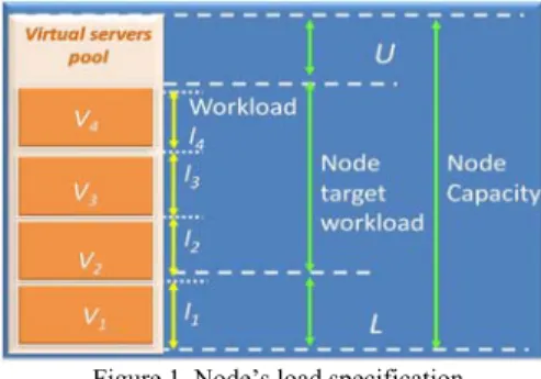
Godfrey et. al. [9] and Rao et. al. [11]. In [8], a virtual server represents a peer in the DHT; that is the storage of data items. In addition, routing takes place at the virtual server level rather than at the physical node level. Each physical node has a pool of VSs as seen in figure 1. Load balancing could be achieved by migrating VSs from heavily loaded physical node to lightly loaded physical node. One main advantage of using VSs for balancing the load is that approach does not require any changes to the underlying DHT. In fact, the transfer of a virtual server can be implemented simply as a peer leaving and peer joining the system. In [11], Rao et. al. proposed three simple and static load balancing schemes: “ one-to-one”, “one-to-many” and “many-to-many”. Godfrey et. al. combines both “one-to-many” and “many-to-many” schemes and uses them in different scenarios [9]. Clustered VSs scheme is presented in [12] that optimized the basic VS framework to reduce the overhead involved in the VS framework. However, VSs cannot be moved, and therefore, the scheme cannot respond to dynamic changes in network conditions. This paper focuses on the design and analysis of P2P load balancing algorithm based on stochastic analysis [23, 24] and based on the VSs concept [8].

C. Challenges: P2P Load Balancing

Load balancing techniques in P2P systems are facing challenges coming from the characteristics of these systems. First, the size of the P2P system is large that means a scalable load balancing technique is required. Second, dissimilar to the traditional systems, nodes of a P2P system are not replicas and requests cannot be executed in any node. If nodes have dated, inaccurate information about the state of other nodes, due to random communication delays between nodes, then this could result in unnecessary periodic exchange of loads among them. For example, an overloaded node removes

some of its virtual servers. However, such simple deletion will cause the problem of “load thrashing1_{”, for}

the removed virtual servers may make other nodes overloaded. Consequently, this paper proposes a stochastic P2P load balancing algorithm that approximately determines the minimum amount of time to change the node’s state from overloaded to underloaded and vice-versa. Comparing that time with the required time to migrate virtual servers enable us to come to a careful decision. Accordingly, the proposed algorithm undoubtedly avoids the load thrashing. To the best of the author’s knowledge, there is no any load balancing algorithm for the P2P system based upon the following stochastic analysis.

III.LOADSHARINGALGORITHM A. Model

This paper considers a P2P system consisting of M physical nodes (peers), denoted by Pi,

1

≤

i

≤

M

. Each

peer can be modeled as a queuing system, such as M/M/1, M/D/1, etc. Each physical node Pi has a capacity

Ci that corresponds to the maximum amount of load that

it can process per unit of time. Nodes create virtual servers (VSs), which join the P2P network. Therefore, it can own multiple noncontiguous portions of the DHT’s identifier space. Each virtual server participates in the DHT as a single entry (e..g routing table). Moreover, each virtual server stores data items whose IDs fall into its responsible region of the DHT’s identifier space. As seen in fig. 1, a node Pi might have n VSs v1, v2, …, vn;

where n= VSset.size. Each vj has load lj; (for j=1, ..n).

The load of peer Pi in a unit of time is Li = l1+l2 + ...+ln.

The utilization of a node’s Pi is Li/Ci. From the

perspective of load balancing, a virtual server represents certain amount of load (e.g. the load generated by serving the requests of the data items whose IDs fall into its responsible region) [25]. To avoid fluctuations in workload nodes should operate below their capacity. If a node finds itself receiving more load Li than the upper

target load U (i.e. (Li/Ci)>U), it considers itself

overloaded. A node Pi also has load Li less than L is

considered to be underloaded. An overloaded node is not able to store objects given to it route packets, or carry out computation, depending on the application.

Definition 1.

A node Pi is in one of the following state as follows

⎪ ⎩ ⎪ ⎨ ⎧ < ≤ ≤ < = i i i i Q U if Overloaded U Q L if Normal L Q if d Underloade S

Clearly the state space Qi consists of non-negative integers sub-divided into three disjoint regions [0, L), [L,U] , and (U,

∞

) corresponding to underloaded, normal, and overloaded state respectively.

1_{Load thrashing is a condition when the load balancing algorithm is}

engaged in moving virtual servers back and forth between nodes.

Figure 1. Node’s load specification

A P2P system is defined to be balanced if the sum of the load Li of a physical node Pi is smaller than or equal to

the target load of the node for every node Pi,

1

≤

i

≤

M

in the system. When the system is imbalanced, the goal of a load balancing algorithm is to move VSs from overloaded node to underloaded one with minimum load transfer overheads.

The amount of overload to be transferred from the overloaded node Pi;

1

≤

i

≤

M

is a random variable

denoted by A is given by ⎩ ⎨ ⎧ − > = − = Otherwise U Q if U Q U Q p A i i i i 0 } , 0 max( ) (

Similarly, the amount of underload that can be accepted at the underloaded peer Pi;

1

≤

i

≤

M

is a random

variable denoted by B is given by

⎩ ⎨ ⎧ − < = − = Otherwise L Q if Q L Q L p B i i i i 0 } , 0 max( ) ( Definition 2.

Let {Q(t) ; t≥0} be a stationary2 _{stochastic process with}

state space consisting of non-negative integers. Let Si

and Sj be two distinct non-negative numbers. The First

Passage Time (FPT) between states Si and Sjis denoted

by FPT(Si,Sj ), is given by ⎩ ⎨ ⎧ = ≠ = = = S S if S S if S Q S t Q t S S FPT i j i i j j i 0 )} ) 0 ( , ) ( ; { inf ) , (

It is a random variable which measures the minimum amount of time needed to reach state Sj from state Si. We

note that because the same stochastic process Q(t) is stationary, translating the above events by a fixed amount of time has no effect upon the probability distribution of FPT(Si,Sj ). In fact, a first passage time

from state Si to state Sj can be divided into two parts,

namely the first transition out of state Si (say Sk )

followed by the first passage from Sk to Sj.

Assume that, i<j; since changes of state have unit magnitude in a birth and death of load, then

FPTij = FPTik + FPT kj i<k <j ; k=i+1, i+2 , …, j-1thus

∑

− = + < = 1 , 1 j i k k k ij FPT i j FPT (1) Similarly, if i>j

∑

− = + > = 1 1, i j k k k ij FPT i j FPT (2) 2_A

stationary stochastic process has the property that the joint

distribution don not depend on the time origin. The stochastic process

{Q(t); t∈ℑ} is called stationary if ti∈ℑ and ti+s ∈ℑ, i=1, 2, …, k (k is

any positive integer), then {Q(t1), …, Q(tk)} and {Q(t1+s), …, Q(tk+s)}

Let Hij(t)= P{FPTij ≤ t} and considering that the

summands in both equation (1) and (2) are independent. Thus, if we apply Laplace transformer

) ( ~ 1 1 , ~ s H H j i k k k ij

∏

− = +

= for Hij(t), then we can show that:

) ( ; ) 1 , , ( ~ ) ( ~ 1 Upward j i k k s H s H j i k ij =

∏

+ < − = (3) ) ( ; ) , 1 , ( ~ ) ( ~ 1 Downward j i k k s H s H i j k ij =

∏

+ > − = (4) Clearly the distribution of the first passage time of unit downward is independent of starting state while the distribution of the first passage time of unit upward depends upon starting state.

B. Load Sharing Edge

The aim of this section is to study the FPT of the transition from normal state to overloaded, overloaded to normal, underloaded to normal, etc. For each transfer pair, FPT will be computed to predicate the future behavior of the transfer pair before the load transfer (i.e. virtual server migration) decision is taken.

Definition 3.

Let [Q(t), R(t)] be a transfer pair with Q(t)=X and R(t)=Y, where X>U and Y<L.The Load Sharing Edge LSE between Q and R is a random variable E(X,Y) which is defined as follows:

E(X,Y) = min {FPT(X,U), FPT(Y,L)}

Where, FPT(X,U) is the first passage time to move from state X to state U and FPT(Y,L) is the first passage time to move from state Y to state L.

LSE is the period of time within which the overloaded node must complete transferring load to the underloaded node before the overloaded node identifies that is unnecessary to transfer load or the underloaded node becomes ineligible to receive a transferred load. Assume the load transfer time is denoted by ∆. It is the time needed to package and send the load (i.e. the least loaded virtual server that will release overload) to sink R. Thus, the load transfer must be initiated only if LSE >∆. Since LSE is a random variable we need to formulate the transfer criterion in terms of probabilities. Assume the probability that LSE exceeds ∆ is P{E(X,Y) >∆}. Therefore, the load transfer must be initiated if P{E(X,Y) >∆} is large. These considerations led to the formulation of a class of rules so called Quantile rules. The quantile of a probability distribution function is defined as follows:

Definition 4.

Let F(t), t≥0 be the probability distribution function of a non-negative random variable X. Let 0<β<1. The β -quantile of F is a non-negative real number q_βsatisfying

. } { , ) ( 1−F qβ = β P X ≥qβ =β

From definition 4, the β-quantile rule for load transfer was introduced.

Definition 5.

Given a transfer pair [Q(t), R(t)] and a load transfer time is ∆. Also, for 0<β<1, let q_βbe the β-quantile of the probability distribution of the LSE between Q(t) and R(t). Then the load transfer is initiated only if q_β>∆. The proposed algorithm in this paper uses a β-quantile rule before transferring load and ensures that 1≥P{E(X,Y) ≥∆} ≥β. In general β can be taken 0.90 or large.

The probability distribution of the random value LSE is given as follows . 0 } ) , ( { ) , ; (t X Y = P E X Y ≤t for t≥ Pe

Thus, the probability distribution function of the load sharing edge LSE between pair Q(t) and R(t) is given by

)]. , ; ( 1 [ )] , ; ( 1 [ 1 ) , ; (t X Y F t X U G t Y L Pe = − − × −

Where F(t; X,U) and G(t; Y,L) are the probability distribution of the first passage time from X to U and from Y to L in the queues {Q(t)}, {R(t)}, respectively. Each node is modeled as M/M/1 queue, in which processes arrive according to a Poisson process with mean arrival rate λ, then processed with exponential service time [23, 24] and with mean service rate µ. Lemma 1.

Assume constant birth rates λ = λ0=λ1=… and death

rates µ=µ0=µ1=…, then the probability distribution

function is

Hk+1,k( . ) = H1,0( . ) k=0,1,…

Proof:

FPTk+1,k is the time that elapses before the cumulative

number of deaths first exceeds the cumulative number of births when X(0)=k+1. Also, the value of Hk+1,k( . ) do

not depend on X(0), [23, 24]. Lemma 2.

The Laplace-Stieljes transform of the probability distribution function of the first passage time from state k to state 0 in an M/M/1 queue is

(

)

k k s s s H ⎥ ⎥ ⎦ ⎤ ⎢ ⎢ ⎣ ⎡ _{+ + − + + −} = λ λµ µ λ µ λ 2 4 ) ( ~ 2 0 , (5) Proof:

Assume that, the first passage time FPTij can be

expressed as ⎪⎩ ⎪ ⎨ ⎧ − = + = + = − + 1 ) ( 1 ) ( 1 , 1 1 , 1 1 _{FPT if X s i} i s X if FPT S FPT j i j i ij

Where S1 is the time of the first transition. Assume that

Hij(t)= P{FPTij ≤ t}, as well FPTij can be upward or

downward after the first transition S1. Using theorem

4-7, [23, 24], Hij(t) can be expressed as follows

∫

∫

− + − + − + − + − = t x j i i t _x j i i ij t H t xe dx H t xe dx H i i i i 0 ) ( , 1 0 ) ( , 1 ( ) ( ) ) ( λ λ µ µ λ µ (i)

Taking Laplace-Stieljes transform on both side of equation (i) and use the convolution property, then the following equation can be obtained:

j j j i i j i i j i s s H s H s H µ λ µ λ + + + = + − ( ) ~ ) ( ~ ) ( ~ 1, 1, , (ii) Thus,

Set i=1, and j=0 0 0 0 , 0 0 0 , 2 0 0 , 1 ) ( ~ ) ( ~ ) ( ~ µ λ µ λ + + + = s s H s H s H (iii)

From lemma 1, λ = λ0, µ=µ0and from equation (4)

j i s H s H i j k k k j i =

∏

> − = + ; ) ( ~ ) ( ~ 1 , 1 , . Thus,

(

)

2 0 , 1 1 , 2 0 , 1 0 , 2 ( ) ~ ) ( ~ ) ( ~ ) ( ~ _{s H s H s H s}

H = × = from equation (iii),

we obtain the following quadratic equation

[

~ ( )

]

( ) ~1,0( ) 0 2 0 , 1 − + λ + µ + µ = λ H s s H s (iv)

Equation (iv) has two solutions, we consider the solution which satisfies that ~ _{( ) 1}

0 , 1 s ≤ H

(

)

1 ) ( ~ ; 2 4 ) ( ~ 0 , 1 2 0 , 1 ≤ ⎥ ⎥ ⎦ ⎤ ⎢ ⎢ ⎣ ⎡ _{+ + − + + −} = s s H s s H λ λµ µ λ µ λ , for real. Hence,

_[

_]

K ( ) k k s s s H s H ⎥ ⎥ ⎦ ⎤ ⎢ ⎢ ⎣ ⎡ _{+ + − + + −} = = λ λµ µ λ µ λ 2 4 ) ( ~ ) ( ~ 2 0 , 1 0 , Corollary 1.

The density function of the first passage time from state k to state 0 in an M/M/1 queue is

(

)

(

)

t t I ke t h k k t o k 2 / ) ( , / 2 ) ( ₌ −λ+µ λµ µ λ (6) For t > 0 m; where Ik is the Modified Bessel function of

order k. Proof:

If equation (5) is bona fide Laplace transform, it is the Laplace transform of h(t), [23, and 24]. From Laplace transform, ) ( )} ( {ectf t ₌f s₊c ℘ − _{; set (c=λ+µ) and w=(s+λ+µ);}

So we can write equation (5) as

⎥ ⎥ ⎦ ⎤ ⎢ ⎢ ⎣ ⎡ _{− −} = λ λµ 2 4 ) ( ~ 2 0 , 1 w w w H , [23, 24].

While the Laplace transformation

a a s s t at I 2 2 1( )/} { = + +

℘ , [23] then we can say that the

numerator is the Laplace transform of

( )

I(2t

( )

)/t 2 1/2 1 2 / 1 _λµ

λµ ; thus, H_1,0 =(s) is the Laplace transform of equation (5). So we have

(

)

( ) t t I ke t h t o λ µ λµ µ λ ₂ / ) ( ( ) 1 , 1 + − = . Hence,

₍

₎

( ) t t I ke t h k k t o k 2 / ) ( , / 2 ) ( ₌ −λ +µ λµ µ λ ; t > 0. Lemma 3. (Downward)

The probability distribution of the first passage time form state k to state 0 in an M/M/1 queue is:

( ) ( ) ∑∞ = + + Γ + − = 0 2 ) , 2 ( 0 . 1 ) 0 , ; ( n n k n k _{n k x} k k x H µ λ λµ µ (7)

Where Γ( )is the incomplete Gama function.

Proof:

Assume that the modified Bessel function of order k is

(

)

∑

∞ = ≥ + ⎟ ⎠ ⎞ ⎜ ⎝ ⎛ = 0 2 0 ; )! ( ! 4 / 2 ) ( n n k k x k n n x x x I Set _x = _{2t λµ} . Thus,

₍

₎

∑∞ = ≥ + ⎟ ⎟ ⎠ ⎞ ⎜ ⎜ ⎝ ⎛ = 0 2 0 ; )! ( ! 2 2 ) 2 ( n n k k x k n n t t t I λµ λµ λµ By substitute

into equation (6), we can compute the density function ) ( , t hko as follows: ( )

∑

∞ = − + + − _≥ + = 0 1 2 ) ( , ; 0 )! ( ! ) ( n n k n t o k t k n n t e k t h µ λ µ λµ

From the definition of the probability distribution function, we have

∫

= x k k x h t dt H 0 0 , 0 ,( ) () and

∫

∞ − = x k k x h t dt H ,0( ) 1 ,0() . Thus, ( )

∫

∑

∞ ∞ = − + + − + − = x n n k n t k k _{n n k} dt t e k x H 0 1 2 ) ( 0 ,( ) 1 _{!( )!} λµ µ λ µ .

If we exchange the infinite sum and the integral we get

( )

_∫

_∫

∑

∞ ∞ − + + − ∞ − − = = Γ + − = x i t x n k t n n k x _{n n k} e t dt i x e t dt H ; (, ) . )! ( ! 1 ) ( ( ) 2 1 1 0 0 , λ µ λµ Hence, ( ) ( ) ∑∞ = + + Γ + − = 0 2 ) , 2 ( 0 . 1 ) 0 , ; ( n n k n k _{n k x} k k x H µ λ λµ µ . Lemma 4.

The probability density function of the first passage time of the M/M/1 queue from state 0 to state 1 is

t e t h _{( )=} λ −λ 1 , 0 . Proof: Let j j j i i j i i j i s s h s h s h µ λ µ λ + + + = + − ( ) ~ ) ( ~ ) ( ~ 1, 1, ,

set i =0, j=1 (i.e. there is no service µ₀=0 ) and 0 , 1 , 1 0 01 ) ( ~ ) ( ~ λ λ + = s s h s h j . For

simplicity set λ0=λ. Hence h~0,1(s)= _s+λ;h~1,1=1

λ since

FPT11=0. By computing the inverse of the Laplace

transformation we get: t e t h _{( ) = λ} −λ 1 , 0 . Lemma 5. (Upward)

The probability distribution function of the first passage time of the M/M/1 queue from state i to state j; i < j is

( )

∑

= − − + = j k t r k i j j i t C e k H 1 , ( ) 1 λ (8)

where r_k;1≤ k ≤ j , are j distinct roots of the polynomial of degree j defined recursively as:

2 ); 2 , ( ) 1 , ( ) ( ) , ( ) 1 , ( ; 1 ) 0 , ( , 0 ) 1 ( ≥ − − − + + = + = = = − j j s D j s D s j s D s s D s D s D λµ µ λ λ also, for

₍

₎

k r s k k _{sD s i} i s D r s C j k − = + = ≤ ≤ ) , ( ) , ( , 1 . Proof:

In lemma 4, we have prove

λ λ + = s s h~0,1( ) that is the

Laplace transformation of the probability distribution of the first passage time of FPT01. Assume that

j j j i i j i i j i _s s h s h s h µ λ µ λ + + + = + − ( ) ~ ) ( ~ ) ( ~ 1, 1, , . Set i=k,j=k+1, µ µ µ λ λ λk = k+1= , k = k+1=

µ λ µ λ + + + = + + − + + s s h s h s h k k k k k k ) ( ~ ) ( ~ ) ( ~ 1, 1 1, 1 1 , (i), But, h~k+1,k+1(s)=1 since FPTk+1, K+1=0, ) ( ~ ) ( ~ ) ( ~ 1 , , 1 1 , 1 s h s h s hk− k+ = k−k kk+ . Hence, µ λ µ λ + + + = − + + s s h s h s h k k kk k k ) ( ~ ) ( ~ ) ( ~ 1, , 1 1 , ( )

(

)

[

h s

]

s s h k k k k , 1 1 , ~ 1 ) ( ~ − + − + + = µ λ λ (ii), Using mathematical induction, we can prove that equation (ii) is satisfied for allk ≥ 0. It can be rewritten

as the ratio of two functions N(s,k) and D(s,k) . These functions can be defined as follows:

(

)

1 ) ( 2 , ) ( , ) 1 ( ≥ = ≥ + − = − = k k M k k L L λµ µ λ λ Thus,

[

( )

]

( , 1) ( ) ( , 2); 1 ) , ( 1 ) 0 , ( ; 1 ), 1 , ( ) , ( ≥ − × − − × − = = > − = k k s D k M k s D k L s k s D s D k k s D k s N λ

Where D(s,k) is a polynomial of degree k;k ≥ j. Thus, equation (ii) can be rewritten as follows:

2 , ) 2 , ( ) 1 , ( ) 1 , ( ) , ( ) , ( ) ( ~ , 1 _{+ + − − −} ≥ − = = − k k s D k s D s k s D k s D k s N s hk k _{λ µ λµ} λ

But for general transitions from state i to state j:

j i ≤ ≤ 0 , is ) , ( ) 1 , ( ) 1 , ( ) 2 , ( ... ) 2 , ( ) 1 , ( ) 1 , ( ) , ( ) ( ~ , j s D j s D j s D j s D i s D i s D i s D i s D s hij − × − − × × + + × + = λ λ λ λ

Thus, we can obtain the Laplace transform of the density of the upward transition from state i to state j,

) , ( ) , ( ) ( ~ , _{sD s j} i s D s h i j j i −

=λ by canceling the common terms from

the denominator and the numerator from the above equation.

From the definition

, ) ]( [ ) ( ) ( 0 s s h LT s dt t h LT x = ⎥ ⎦ ⎤ ⎢ ⎣ ⎡

∫

thus ) , ( ) , ( ) ( ~ , j s sD i s D s H i j j i − =λ

It is a relation function in which the numerator polynomial has degree I while the denominator polynomial has degree (j+1) and (i <j). Thus, we can expand H~i,j(s) into a finite sum of partial fractions as

follows: If _D(0,j)=λj_{for all j≥1andλ>0then zero} cannot be a root of D(s,j);j≥1and it can be written in the following form:

) )...( )( ( ) , (s j s r1 s r2 s rj

D = + + + where rk for all k =1 to j are roots of D(s, j)

.

Hence, it can be written as

follows: ⎟⎟⎠ ⎞ ⎜⎜ ⎝ ⎛ + + =

∑

= − j k k k i j j i r s C s C s H 1 0 , ) ( ) ( ~ _λ Where k r s k k j s sD i s D r s C − = − + = ) , ( ) 1 , ( ) ( ;

1

≤

j

≤

k

and j i j i j D i D C _{= = =λ}− λ λ ) , 0 ( ) , 0 ( 0

∑

= − + + = j k k k i j j i _{s r} C s s H 1 , _{( )} 1 ) ( ~ _λ

Accordingly, we can invert the Laplace Transform of the above equation. But, each term in the right hand side is in the form β α β α _, ) (s+

Where α,β are constants. Each term has inverse Laplace transformation

α

e

βt. Hence, ( )

∑

= − − + = j k t r k i j j i t C e k H 1 , ( ) 1 λ Theorem

Let [Q(t), R(t)] be a transfer pair that consists of M/M/1 queues. Let m be the amount of overload and n the amount of underload. Then the probability distribution function of the Load Sharing Edge (LSE)is

( )

(

)

(

)⎥

⎦ ⎤ ⎢ ⎣ ⎡ + Γ + × ⎥ ⎦ ⎤ ⎢ ⎣ ⎡ − =

∑

∑

∞ = + = − 0 2 1 , 2 1 ) , ; ( k k m k L k t r k m n e tmn m Ce n mx P k µ λ λµ µ λ

where, rk,1≤k≤L ; are the roots of the polynomial

defined recursively as L k L L s D L s D s L s D s s D s D s D ≤ ≤ ≥ − − − + + = + = = = − 1 ; 2 ); 2 , ( ) 1 , ( ) ( ) , ( ) 1 , ( ; 1 ) 0 , ( ; 0 ) 1 , ( λµ µ λ λ Also, for

(

)

k r s k k L s sD n L s D r s C L k − = − + = ≤ ≤ ) , ( ) , ( 1 . Proof:

The transfer pair has the probability distribution function

) , ; (ti j

P_e of the LSE; i>U,j<Lwhich is defined by

[1 (;, )]] [*1 (; , )] 1 ) , ; (t i j F tiU G t j L Pe = − − − where m is the

amount of overload (m =i-U), and n is the amount of underload (n =L-j) then [1 (; ,0)]] [*1 (; , )] 1 ) , ; (t mn F t m G t L n L P_e = − − − − for an M/M/1

queue case F(t,m,0) and G(t, L-n, L) have been derived from 3 and 5 respectively. Hence,

( )

(

)

(

)

⎥⎦ ⎤ ⎢ ⎣ ⎡ + Γ + × ⎥ ⎦ ⎤ ⎢ ⎣ ⎡ − =

∑

∑

∞ = + = − 0 2 1 , 2 1 ) , ; ( k k m k L k t r k m n e tmn m Ce n mx P k µ λ λµ µ λ .

Due to the infinite number of terms in the probability distribution Pe(t;m,n)of the LSE in M/M/1, the following lemma will drive a formula for LSE as finite number of terms as follows.

Lemma 6

For a transfer pair [Q(t), R(t)] with an amount of overload m and an amount of underload n, the Mean Load Sharing Edge MLSE(m, n)is

∑

= ⎟⎟⎠ ⎞ ⎜⎜ ⎝ ⎛ − − = L k k k k n _{F r m} r C n m MLSE 1 ) 0 , , ( ~ 1 ) , ( λ

where r₁,r₂,...,r_k,C_kare constants defined in the previous theorem. Also,

(

)

m m s s s F ⎥ ⎥ ⎦ ⎤ ⎢ ⎢ ⎣ ⎡ _{+ + − + + −} = λ λµ µ λ µ λ 2 4 ) ( ~ 2 0 , Proof: Since P_e(t;m,n)=1−

[

1−F(t;m,0)]

] [

×1−G(t;L−n,L)

]

we obtain,

[

F t m

] [

G t L n L

]

dt dt n m t P n m MLSE e

∫

∫

∞ ∞ − − × − = = 0 0 ) , ; ( 1 )] 0 , ; ( 1 ) , ; ( ) , (

From lemma 5, we get

[

F t m

]

dt e C n m MLSE L k t r k n k

∫

∑

∞ = − _{× −} ⎥ ⎦ ⎤ ⎢ ⎣ ⎡ − = 0 1 ) 0 , ; ( 1 ) , ( λ

But the Laplace transform _{LT q s q t dt}

S

∫

∞ = = 0 0 ( ) ) ]( [ and ) ]( [ ) ]( [ 0 α α _{= +} = − _{q s LT q s} e LT s t . Set r then k, = α

∑

= ⎟⎟⎠ ⎞ ⎜⎜ ⎝ ⎛ − − = L k k k k n _{F r m} r C n m MLSE 1 ) 0 , , ( ~ 1 ) , ( λ .

Consequently, it has been observed that for queuing models in which job arrival and processing rates are independent of queue size, such as M/M/1 queues. The distribution of LSE depends only on the amounts of underload and overload. The following algorithm will use the numeric value of the given mean load sharing edge formula that is based upon the following parameters

(

m,n,

λ

i,

µ

i,

λ

j,

µ

j,L,q_β

)

.

C. Algorithm

This section introduces the proposed load balancing algorithm based upon the above analysis. Periodically every T seconds, each overloaded peer transfers the exceeds load to the underlaoded peers (i.e. sender-initiated algorithm). This algorithm imposes a β-quantile rule for transferring load. For each pair (λ, µ) a corresponding β-quantile should be determined while β

must be taken 0.90 or large. The algorithm is shown in the following scenario:

1. The overloaded node Si creates a suitable domain

(group) Di from neighbor nodes to the peer Si. Each

node blongs to Di satisfies Di = {Sj; P(FPTi >tij)

≥0.90 and i≠j}. Where tij is the required

communication delay to send a message form node Si

to Sj plus the required time to reply with load transfer

of certain virtual server from Si to Sj. Also, FPTi is

the first passage time of node Si to tranfer from

overloaded state to normal or underloaded state. Di is

an ordered set with respect to the communication tij.

It is implemented as an order linked list.

2. Thus, Si sends a broadcast messages to all nodes

belonging to the doamin Di. Node Si must receive a

reply from all nodes belonging to Di within the FPTi

time.

3. Node Si selects an underlaoded node Sj∈Di where the

mean load sharing edge MLSE between Si and Sj. if β

q >∆ then transfers load (virtual server) from Si to Sj.

Where pair λ and µ are given, ∆ is the time needed to transfer load less than or equal to A(Sj), β is 0.90 or

large.

4. Repeate step 3 for each underloaded node Sj

belonging to Di whenver FPTi period doesn’t run out

yet.

IV. EVALUATION

This paper implements an event-based simulation to evaluate the proposed load balancing algorithm. It uses several parameters as follows: default number of virtual servers per node (12), number of nodes (4096), system utilization (0.8), Object arrival rate (Poisson with mean arrival time 0.01 sec), average number of objects (1 million), and periodic load balancing period (T=60 seconds). This simulation evaluates the following metric. Load Movement Ratio (LMR), defined as the total movement cost incurred due to load balancing divided by the total cost of moving all objects in the system at once. In case the value of the LMR is 0.1, it infers that the balancer consumes about 10% of its bandwidth to insert objects. The node arrival rate is modeled by a Poisson process, and the lifetime of a node is drawn from an exponential distribution. This simulation ran with two inter-arrival times 10 and 60 seconds, it fixes the steady-state number of nodes in the system to 4096 nodes.

Fig. 2 plots the LMR metric as a function of system utilization, to study the load moved by the proposed load balancing algorithm as a fraction of the load moved by the underlying DHT due to node arrivals and departures. Fig. 2 demonstrates that the load moved by the proposed load balancing algorithm is significantly smaller than the load moved by the underlying DHT especially for small system utilization. In addition, fig. 2 shows that the LMR with node inter-arrival time 10 sec is larger than with node inter-arrival time 60 sec. Fig. 3 verifies the perception that increasing the number of virtual servers decreases considerably the fraction of load moved by the underlying DHT. Fig. 4 demonstrates that increasing

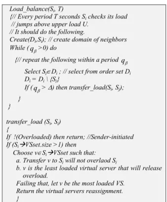
Load_balance(Si, T)

{// Every period T seconds Si checks its load // jumps above upper load U.

// It should do the following.

Create(Di,Si); // create domain of neighbors While (q_β>0) do

{// repeat the following within a period q_β Select Sj∈Di ; // select from order set Di

Di = Di \ {Sj} If (q_β> ∆) then transfer_load(Si, Sj); } } transfer_load (Si, Sj) {

If !(Overloaded) then return; //Sender-initiated If (SiÆVSset.size >1) then

Choose v∈SiÆVSset such that: a.Transfer v to Sj will not overlaod Sj

b.v is the least loaded virtual server that will release overload.

Failing that, let v be the most loaded VS. Return the virtual servers reassignment. }

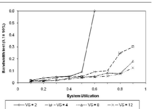
number of virtual servers per node assists load balance at high system utilizations and grants efficient load movements due to low bandwidth lost. Fig. 5 plots the 90-quantile of the load sharing edge (LSE) with system utilization when overload is 5 at source node and underload is 2 at the destination node. It demonstrates that the 90-quantile of the LSE tends to be smaller as system utilization increases. As seen from fig. 5, the 90-quantile of the LSE is 9.94ms thus load can be transferred only if ∆<9.94ms. In addition, increasing the number of virtual servers reduces significantly the 90-quantile that helps in avoiding load thrashing.

V. CONCLUSION

Load balancing among peers is critical and a key challenge in peer-to-peer systems. This paper exhibits a stochastic analysis that avoids the load thrashing and tackles the out-of-date problems due to peer’s state changes during load movement (virtual servers migration). Then, it proposes a load balancing algorithm based on that stochastic analysis. An efficient simulation has been carried out that demonstrates the effectiveness of the proposed load balancing algorithm.

Figure 2. LMR vs. system utilization with two node arrival times.

Figure 3. LMR vs. number of virtual servers with two node arrival times.

Figure 4. Bandwidth lost vs. system utilization with different number of virtual servers per node.

Figure 5. 90-quantile of the LSE vs. system utilization with different number of virtual server per node.

REFERENCES

[1] Shirky C., “Modern P2P Definition,” http://www.

openp2p.com/pub/a/p2p/2000/11/24/shirky1-whatisp2p.html, 2000.

[2] S. Saroiu, et. al., “A Measurement study of Peer-to-Peer

sharing systems,” Proc. Multimedia Computing and Networking Conf. (MMCN, 2002.

[3] I. Sotica, et. al., “Chord: A scalable peer-to-peer lookup

service for Internet Applications,” ACM SIGCOMM’01, August 2001, pp. 149-160.

[4] Antony Rowstron and Peter Druschel, “Pastry: Scalable

distributed object location and routing for large-scale Peer-to-Peer systems ,” in Proc. Middleware, 2001.

[5] S. Ratnasamy, et al. “A Scalable Content- Addressable

Network,” in Proc. ACM SIGCOMM’01, California,

USA

[6] Derk I., et al. “Adaptive load sharing in homogenous

distributed systems,” IEEE Trans. on Soft. Eng., Vol. 12 No 5, Sept. 1986.

[7] A. R. Bharambe, et. al., “Mercury: supporting scalable

multi-attribute range queries,” In Proc. of the Conf. on Applications, Technologies, Architectures, and Protocols For Computer Communication, ACM, New York,2004.

[8] Frank Dabek , et. al. , “Wide-area cooperative storage

with CFS,” Proc. 18th ACM Symp. Operating Systems Principles (SOSP’01), pp. 2020-215, Oct. 2001

[9] Godfrey et. al., “Load balancing in dynamic structured

P2P systems,” Proc. IEEE INFOCOM, 2004.

[10]J. Byers, “Simple load balancing for distributed hash

table,” Proc. Of the 2nd Int. Workshop on Peer-to-peer systems (IPTPS’03), Feb. 2003.

[11]A. Rao et. al., “Load balancing in structured P2P systems,” Proc. Of the 2nd Int. Workshop on Peer-to-peer systems (IPTPS’03), Feb. 2003.

[12]P.B.Godfrey and I. Stoica, “Heterogeneity and Load

balance in distributed hash table,” Proc. IEEE INFOCOM, 2005.

[13] Jie Li, Hisao Kameda, “A decomposition algorithm for optimal static load balancing in Tree hierarchy network configurations,” IEEE Trans. On Parallel and Distributed Systems, Vol. 5, No.5, 1994.

[14]T.L. Casavant, and J.G. Kuhl, “A taxonomy of scheduling

in general-purpose distributed computing systems,” IEEE Trans. on Software Engineering, vol. 14, no. 2, pp. 141-154, Feb., 1988.

[15]N. G. Shivaratri, et. al. , “Load distributing for locally

distributed systems,” Computer, vol.25, no.12, pp.33-44, Dec 1992

[16]Goscinski, A., “Distributed Operating System: The logical

design,” Addison-Wesly, 1991.

[17]S. Zhou, “A Trace-Driven Simulation Study of Dynamic

Load Balancing,” IEEE Transactions on Software Engineering, vol. 14, no. 9, pp. 1327-1341, Sept., 1988.

[18]D. L. Eager, et.al., “A comparison of receiver-initiated

and sender-initiated adaptive load sharing,” SIGMETRICS Performance Evaluation Review 13, 2, Aug. 1985.

[19]P. Kruger, and N. G. Shivaratri, “Adaptive location

policies for global schedule,” IEEE Soft. Eng., Vol 20, 432-443, June 1994.

[20]S. Zhou, et.al., “Utopia: a load sharing facility for large,

heterogeneous distributed computer systems,” Software-Practice and Experience. Dec. 1993, pp. 1305-1336.

[21]S. P. Dandamudi, and K. C. Lo, “A Hierarchical Load

Sharing Policy for Distributed Systems,” in Proc. of the 5th Int. Workshop on Modeling, Analysis, and Simulation

of Computer and Telecommunications Systems, MASCOTS. IEEE CS, Washington, DC, 1997.

[22]Heyman, Daniel P., “Stochastic models in operation

research,” vol. I, MxGraw-Hill Inc. 1982.

[23] Hisashi kobayshi, “Modeling and Analysis: An

Introduction to system performance evaluation methodology,” Addison-Wedley, 1978.

[24]Hisashi kobayshi , et. al., “System modeling and analysis:

foundations of system performance evaluation,” Prentice Hall 2009.

[25]Zhu Y. and Hu Y.,”Efficient, Proximity-aware Load

Balancing for DHT-based P2P Systems,” IEEE Trans. On Parallel and Distributed Systems, Vol. 16, No. 4, 2005

Khaled Ragab is an assistant professor at

Department of Computer Science, College of Computer and Information Technology, King Faisal University, Saudi Arabia. Moreover, he is on leave assistant professor of Computer Science at Department of Mathematic, Computer Science division, Ain Shams University. He joined Department of Computer Science, Tokyo University in 2005 as postdoctoral position. He was born in 1968 and received his B.Sc., M.Sc. degrees in Computer Science from Ain Shams University, Cairo, Egypt in 1990, 1999, respectively and Ph.D. degree in Computer Science from Tokyo Institute of Technology in 2004. He has worked in Ain Shams University, Cairo Egypt in 1990-1999 as assistant lecturer. He has worked as research scientist in Computer Science Dept., Technical University of Chemnitz, Germany in 1999-2001. His research interests include autonomous decentralized systems, Peer-to-Peer Systems, Overlay Networks, Load Balancing, Web-services and application-level