Robust TV Stream Labelling with Conditional Random
Fields
Abir Ncibi, Emmanuelle Martienne, Vincent Claveau, Guillaume Gravier,
Patrick Gros
To cite this version:
Abir Ncibi, Emmanuelle Martienne, Vincent Claveau, Guillaume Gravier, Patrick Gros.
Robust TV Stream Labelling with Conditional Random Fields.
MMEDIA - 5th
In-ternational Conference on Advances in Multimedia, Apr 2013, Venise, Italy.
pp.88-95, 2013,
<
http://www.thinkmind.org/download.php?articleid=mmedia 2013 4 40 40094
>
.
<
hal-00844640
>
HAL Id: hal-00844640
https://hal.inria.fr/hal-00844640
Submitted on 20 Oct 2016
HAL
is a multi-disciplinary open access
archive for the deposit and dissemination of
sci-entific research documents, whether they are
pub-lished or not.
The documents may come from
teaching and research institutions in France or
abroad, or from public or private research centers.
L’archive ouverte pluridisciplinaire
HAL
, est
destin´
ee au d´
epˆ
ot et `
a la diffusion de documents
scientifiques de niveau recherche, publi´
es ou non,
´
emanant des ´
etablissements d’enseignement et de
recherche fran¸
cais ou ´
etrangers, des laboratoires
publics ou priv´
es.
Distributed under a Creative Commons Attribution - NonCommercial - NoDerivatives 4.0
International License
Robust TV stream labelling with Conditional Random Fields
Abir Ncibi∗, Emmanuelle Martienne†, Vincent Claveau‡, Guillaume Gravier‡ and Patrick Gros∗
∗INRIA †IRISA-Univ. of Rennes 2‡IRISA-CNRS
Campus de Beaulieu, F-35042 Rennes, France Email: [email protected]
Abstract—Multi-label video annotation is a challenging task and a necessary first step for further processing. In this paper, we investigate the task of labelling TV stream segments into programs or several types of breaks through machine learning. Our contribution is twofold: 1) we propose to use simple yet efficient descriptors for this labelling task, 2) we show that Conditional Random Fields (CRF) are especially suited for this task. In particular, through several experiments, we show that CRF out-perform other machine learning techniques, while requiring few training data thanks to its ability to handle the different types of sequential information lying in our data.
Keywords-Conditional Random Fields, video-stream la-belling, TV segmentation, robust descriptors, sequentiality.
I. INTRODUCTION
Many digital TV channels have emerged in the recent years, making large amounts of video streams available. Yet, any new service based on these streams, such as video retrieval, information extraction, repurposing, requires, as a first step, to be able to structure the video flow into meaning-ful elementary units. In practice, the process of video stream structuring requires two main tasks: (1) a segmentation task that consists in detecting program boundaries, and (2), a labelling task that consists in giving each program a label describing its type or content.
Several studies [1]–[4] have already dealt with this issue. However, their main drawback is that their labelling pro-cesses chiefly rely on program information provided by the channels, on some reference databases, or on TV program guides. They all have underlined the limits of using such an external knowledge which is sometimes inaccurate or in-complete. In particular, TV guides don’t contain information for small programs like commercials. Moreover, such TV guides are not always available. In this paper, to avoid this pitfall, we explore a different approach based on supervised machine learning. Of course, such an approach also requires some expert knowledge to build a training set, but we assume that this supervision is more easily available that a complete program information. More precisely, our goal is to investigate the use of a specific machine learning technique for the labelling task, namely the conditional random fields (CRF), which are known to be suited to handle sequences. In that respect, our objective is manifold; We show that: 1 – CRF are efficient to induce programs labels, and out-perform other standard machine learning techniques;
2 – these good results can be obtained with few data and simple but robust descriptors;
3 – this good performance can be theoretically explained by the CRF’s capability to use contextual relationships among a sequence of programs.
The remainder of this paper is organized as follows: Next section is an overview of related work. In Section III, basic information about conditional random fields and their learning algorithms are presented. Then, in Section IV, we detail our experimental setting, including the datasets used, the features and the evaluation measures. Sections V, VI and VII report the experiments we performed. Finally, we conclude in Section VIII.
II. RELATED WORK
To our knowledge, [1] are the first who proposed a complete solution for the video stream structuring problem. Their approach requires a reference database containing different kinds of breaks that are manually annotated. Breaks that repeat in the video stream are detected by matching the video stream with the breaks included into the reference database. If the video stream contains a new break that is not in the database, this new break is added to the database to update it. The main drawback of this method is its dependency to the reference database. Indeed, the latter has to be created for each channel and updated periodically to take into account all the breaks broadcasted by this channel. Another approach is proposed by [3] and consists in modelling program schedules by contextual hidden Markov models, that are able to predict all the possible schedules for a particular day. This approach gives good results in terms of precision of the prediction, but requires many annotated learning data. Another method developed by [4] uses an inductive logic programming tool to identify two classes of broadcasts: Programs and breaks. The drawbacks of this approach are twofold: (1) it requires at least seven days of manually annotated programs and (2) it is not able to identify different kinds of breaks.
In this paper, we focus mainly on the labelling task. We suppose that the video stream has been divided, manually or automatically, into sequences of video segments. We propose a robust approach that uses CRF to label all the resulting video segments. The highlights of our method are: (1) each
segment is described with robust descriptors that are very easy to compute, and (2) the use of CRF allows for building an efficient model that predicts the types of the segments by taking into account the sequentiality of the data and the relationships between neighbouring segments.
CRF have been successfully applied to text processing, such as part-of-speech tagging [5], [6] or shallow text parsing [7]. They have also been used in video processing for detecting semantic events [8], [9] or identifying players in sports videos [10]. For all these tasks, CRF proved high efficiency and over-classed other probabilistic models, espe-cially generative models like hidden Markov models (HMM) [11], [12] and other discriminant models like maximum entropy Markov model (MEMM) [13].
III. CONDITIONALRANDOMFIELDS:BASIC CONCEPTS AND RELEVANT ALGORITHMS
A. Basic concepts
Conditional random fields [13] are undirected graphical models which aim at model a probability distribution of annotations y conditioned on known observations x
based on labelled examples. CRF are defined as follows: We assume G(V, E) an undirected graph (graph of independence) whereV are vertices of the graph andEare edges of the graph. X and Y are two random fields over respectively the set of observations and the associated set of labels. For each vertex v ∈V, it exists a random variable
Yv in Y. (X,Y) is called a conditional random field when
each random variable Yv depends only on observations X
and its neighbours in the graphG. Based on this condition and according to the fundamental theorem of random fields (Hammersley and Clifford, 1971), the conditional probability of an annotation y given an observation x is written in terms of potential functions ψc over all cliques
of the graphG: p(y|x) = 1 Z(x) Y c∈C ψc(yc, x) where:
• C is the set of all cliques of the graph G(completely connected subgraphs).
• yc are configurations of random variables over vertices
of the cliquec.
• Z(x)is a normalization factor. B. Linear-chain CRF
The main use of CRF in the literature, mainly in natural language processing, is labelling sequences. In this case, the graph of independenceGis a first-order linear chain (as the one shown on Figure 1).
In this graph:
• cliques are adjacent edges and vertices of the graph.
Figure 1. Graphical representation of a sequential CRF
• each label depends only on the previous and the next labels and the entire observations sequencex.
For linear CRF, [13] the potential function ψc can be
written as an exponential of weighted functions over the two types of cliques of the graphGas follows:
P(y|x) = 1 Z(x)exp k1 X k=1 n X i λkfk(yi, x) + k2 X k=1 n X i µkgk(yi−1, yi, x) ! (1) where:
• Z(x)is the normalization factor:
Z(x) =X y exp k1 X k=1 n X i λkfk(yi, x) + k2 X k=1 X i µkgk(yi−1, yi, x) ! (2)
• f andg are called features functions. The f functions characterize local relations in terms of labels and links the current label at position i to the sequence of observations x; The g functions describe transitions between the graph vertices (states) and are defined for each pair of labels (or states) at position i and i−1
and the sequence of observations.
• k1,k2,n are respectively: number of features functions f,number of features functions g and the size of the sequence of labels to be predicted.
Functions inf andgare generally binary functions which show the occurrences of particular combinations of label(s) and observation(s). These functions are fixed by the user, they reflect the knowledge of the user on the application field. Each function is applied to all the positions of the sequence. For instance, let’s definef(xi, yi) which relates
the current observation xi to its current label yi. If we
apply this function to all couples of labels and observa-tions in the sequence, it will generate |x| × |y| functions features. Let’s consider the sequence of observations x = (15s,10m,10s,1h), where each observation is the duration of the corresponding program, and its associated sequence of labelsy = (commercial, trailer, commercial, program). We also suppose that we fix two functions f(xi, yi) and
g(yi, yi−1). At position i = 3, the following feature func-tions are generated:
f(xi, yi) = 1 if xi= 10sandyi=commercial 0 else g(yi, yi−1) =
1 ifyi=commercialandyi−1=trailer
0 else
Features functions are associated with weightsλk andµk
that estimate the importance of information given by each feature function.
The conditional nature of CRF allows for relaxing the as-sumption of observations conditional independence fixed in the HMM, and allows for neighbourhood interactions among the observed data. CRF also avoid the label bias problem met with the HMM (or extensions like MEMM). This prob-lem is caused by the fact that the probability mass received byyt−1 must betransmitted to yt(at time t) regardless the
corresponding observation xt (for the interested reader, a
good illustration of the label bias problem is presented by [13]). CRF are not impacted by such considerations since the way adjacent pairs yt and yt−1 influence each other is not directed and is determined by input featuresx.
C. Learning and inference with CRF
Learning CRF models consists in estimating the vector of parameters θ = (λ1, λ2, ...., λk1, µ1, µ2, ..., µk2) given a training set D = (x(i), y(i))i=N
i=1 which maximizes the log-likelihood of the model:
Lθ= N
X
i=1
log(pθ(y(i)|x(i)))
This function is concave, guaranteeing convergence to the global maximum. This optimization can be resolved by traditional iterative scaling learning algorithms such as the improved iterative scaling (IIS) algorithm [14] but it has been proved that the Limited memory BFGS (L-BFGS) quasi-Newton method [15] converges much faster to estimate the parametersθ. The advantage of L-BFGS is that it avoids the explicit estimation of the Hessian matrix of the log-likelihood by building up an approximation of it, using successive evaluations of the gradient.
After this step of training, applying the CRF consists in finding the most probable sequence of labels y∗ given an unseen sequence of observationsx:
y∗= arg max
y
pθ(y|x)
As for other stochastic methods, y∗ is generally obtained with a Viterbi algorithm, which calculates the marginal probability of states at each position of the sequence, using a dynamic programming procedure.
IV. EXPERIMENTAL SETTING
In this section, we present the data we used for the experi-ments that were conducted to evaluate CRF, as well as other machine learning algorithms, on video stream labelling.
A. Data
In our experiments, we used a TV stream containing three weeks of broadcasts. Within this stream, each segment was manually identified and given a label corresponding to its type: Program or break. Four additional types have also been used to distinguish between different kinds of breaks: trailer, commercial, sponsorships and jingle. Two datasets were produced from this stream, each dataset resulting from the application of a particular segmentation method:
• A manual segmentation method which identifies pre-cisely the beginning and the end of each broadcast. This segmentation will be useful for evaluating the relevance of CRF on the labelling of a perfectly segmented video stream. In this case, a video segment is equivalent to a program (movie, TV serie, talk-show, etc) or a break (commercial, trailer...). 7,591 video segments were extracted using this manual segmentation method. • An automatic segmentation method that aims at evaluat-ing CRF for the labellevaluat-ing in a more realistic settevaluat-ing. The automatic segmentation method we used is based on the detection of repeated segments [16]. Applied to TV streams, this method tends to over-segment the stream: 48,544 video segments were detected. By examining the result of the segmentation, we observe that each broadcast (corresponding to a unique segment with the manual segmentation method) is divided into several segments, each segment having a short duration. The distribution of the segments over the different types, inside both datasets, is shown on Table I.
Label Manual segmentation Automatic segmentation Program 1,506 22,557 Trailer 1,290 4,075 Commercial 1,050 18,089 Sponsorship 1,714 2,201 Jingle 2,031 1,622 Total 7,591 48,544 Table I
DISTRIBUTION OF THE SEGMENTS OVER THE DIFFERENT TYPES
B. Descriptors
Within both datasets, each video segment is described by three descriptors:
• its duration: we distinguish between ten possible values, each value being an interval:[0-15s[, [15s-30s[, [30s-45s[, [45s-1min[, [1m-15m[, [15m-30m[, [30m-1h[, [1h-2h[, [2h-4h[;
• the moment in the week it was broadcasted: business day, off-day or weekend;
• the period in the day it was broadcasted: morning, noon, afternoon, evening, night.
These features are robust since they are very easy to compute, and they do not depend on the quality of image
or sound signal of the stream. Some examples of segments with these features and their labels are shown in Table II.
Segment Moment in Period in Duration Label (class) the week the day
Seg15 Business day morning [10s,15s[ commercial
Seg16 Business day morning [0s,10s[ trailer
Seg17 Business day morning [0s,10s[ jingle
Seg18 Business day afternoon [15min,30min[ program
Seg19 Business day afternoon [10s,15s[ commercial
Table II
EXAMPLES OF SEGMENTS WITHIN THE DATASETS,WITH THEIR
FEATURES AND LABELS
C. Labelling tasks and evaluation measures
For all the experiments, the first two weeks of a dataset were used to train and construct the labelling model, and the last third week to test and evaluate this model. Two kinds of labelling tasks have been considered:
• a binary labelling task in which a segment is either a program or a break (i.e.there is no distinction between different kinds of breaks);
• a multiple labelling task in which a distinction is made between different kinds of breaks. Consequently, five labels are used: Program, commercial, sponsorship, trailer or jingle.
In the experiments reported in the next sections, the performance is evaluated on the test sequences by comparing the labels produced by the technique with those from the ground-truth. Different evaluation measures are used. As a global measure, we compute the accuracy rate, that is, the proportion of correctly labelled segments in the test streams. For each label, we also evaluate the recall, precision and f-score, and we then compute a weighted average over the labels (weighted according to the amount of segments of each class). Note that the weighted average recall is equivalent to the accuracy rate that we use as a global measure.
D. Video stream labelling with CRFs
To use efficiently CRF, we consider that a sequence groups together all the segments of a day of broadcasting. We have 15 sequences (i.e.the first two weeks) for learning the labelling model and 8 sequences (i.e.the last third week) for testing the model. In a sequence, observations are the vectors of features and labels are the types of the segments. To learn the labelling model, appropriate features func-tions must be chosen to express the dependencies that may exist in a sequence between observations or labels. In our experiments, we used the tool CRF++1. In this tool, feature functions are defined in atemplate filewhere:
1http://crfpp.googlecode.com/svn/trunk/doc/index.html
• feature functionsf are equivalent tounigram templates that describe relationships between the current label and the observations in the sequence (see Section III-A); • feature functionsg are equivalent tobigram templates
that describe only the relationships between two suc-cessive labels (see Section III-A).
In Section VII, we presents some results obtained with different templates.
Each experiment was performed on both datasets. To highlight the efficiency of CRFs in sequential data labelling, we compare the results obtained by CRFs with the results obtained by different non sequential classification methods (SVM, Naive bayes, Random Forest) for the same labelling task. For each method, two settings are presented. The first one use a naive description in which only the current observation is considered (noted as simple hereafter). The second one (notedcontextual) takes into account the context of the observations by adding the features of the surrounding observations in the description of the current segment. Different size of context have been tested; here, we report the ones yielding the best results, that is when considering the 2 previous and two next segments. We also compare CRFs to HMMs to study the impact of the label context that is also taken in account by CRFs. To the contrary of CRF, HMM only take into account the current observation of the segment to be labelled. To complete this comparison, we also indicate the results of two baselines:
• Baseline1 where only the most frequent label is pre-dicted;
• Baseline2 which uses a features function which con-siders only the duration of the current segment to be labelled. We choose this baseline because duration is the most discriminant feature.
Again, the experiments are performed on both manually and automatically segmented datasets.
V. RESULTS ON THE MANUAL DATASET
This section is dedicated to the results obtained with the manually segmented stream. In the first part, we summarize the results obtained by CRF and other classification methods. In the second part, we focus on the detailed results obtained by CRF on binary and multiple labelling.
A. Global results on the manual dataset
Results are presented on Tables III and IV. The best results for SVM, reported hereafter, were obtained with a RBF kernel andγset to 0.1. For the results, we attribute to each label a weight that is proportional to its frequency in the learning dataset. Then, we calculate weighted averages of recalls, precisions and F-scores for each predicted label. From these results, several points are noteworthy. First, the task of binary labelling seems easy enough to yield high score with the baseline techniques. Secondly, the difference between the simple and contextual settings of the usual
Accuracy - Precision F-score Recall (%) (%) (%) CRF 95.66 95.63 95.63 HMM 88.79 90.2 89.2 SVM simple 86.3 85.4 85.2 N.Bayes simple 86.6 87 86.8 R.Forest simple 87.1 88.3 87.5 SVM contextual 94.9 94.8 94.8 N.Bayes contextual 89.4 91.0 89.9 R.Forest contextual 94.9 94.8 94.8 Baseline1 79.48 63.16 70.39 Baseline2 87.37 86.66 86.53 Table III
PERFORMANCE FOR THE BINARY LABELLING TASK WITH THE MANUAL
DATASET,USINGCRFAND VARIOUS CLASSIFICATION METHODS
machine learning algorithms underlines the importance of taking the context of the current observation into account as it is naturally done with CRF. Thirdly, the label context, naturally taken into account by HMM and CRF, seems also beneficial for the performance.
Accuracy - Precision F-score Recall (%) (%) (%) CRF 84.08 85.13 84.54 HMM 74.52 53.82 49.22 SVM 59.5 64.6 56.5 N.Bayes 59.6 62.8 56.5 R.Forest 58.7 61.3 55 SVM contextual 76.1 76.8 75.8 N.Bayes contextual 68.6 69.6 68.8 R.Forest contextual 74.9 75.8 74.6 Baseline1 27.36 7.49 11.76 Baseline2 64.3 66.2 64.8 Table IV
PERFORMANCE FOR THE MULTIPLE LABELLING TASK WITH THE
MANUAL DATASET,USINGCRFAND VARIOUS CLASSIFICATION
METHODS
The multiple labelling task is more difficult, resulting in lower performance. Here again, the importance of taking the context of the current observation into account appears clearly. As it is suggested by the HMM results, the context of the label is not enough to cope with these more complex data. Yet, the CRF model, which takes both contexts into account yields the better results and over-performs any other technique.
Finally, these results highlight the two following interest-ing points:
• using features functions, CRF are the most competitive method for the task of video sequence labelling. • robust descriptors are discriminant enough to label the
manual dataset.
B. CRF results on the manual dataset
In order to analyse the errors, we report detailed results for the CRF in Tables V and VI. CRF have interesting results in
Number of Recall Precision F-score segments (%) (%) (%) Inter-Program 1.184 97.52 97.03 97.27
Program 564 88.47 90.23 89.34 Weighted average 95.66 95.63 95.65
Table V
DETAILED PERFORMANCE FOR THE BINARY LABELLING TASK WITH
THE MANUAL DATASET USINGCRF
binary labelling: both programs and breaks are identified by the learned model. Breaks are better identified than programs because they are more numerous in the learning dataset and are characterized by their short duration.
Number of Recall Precision F-score segments (%) (%) (%) Program 564 88 92.31 90.10 Trailer 381 88.47 90.23 89.34 Jingle 752 85.37 81.87 83.53 Commercial 309 87.37 82.56 84.9 Sponsorship 742 76.17 81.43 78.71 Weighted average 84.08 85.13 84.54 Table VI
DETAILED PERFORMANCE FOR THE MULTIPLE LABELLING TASK WITH
THE MANUAL DATASET USINGCRF
In multiple labelling, CRF are still able to predict labels with a F-score equal to 84.54%. Programs are the best predicted class with 92.31% precision and 90.10% F-score.
VI. RESULTS ON THE AUTOMATIC DATASET
The automatic segmentation technique used to produce what we refer as the automatic dataset tends to over-segment the stream, as a sequence the programs or breaks are generally divided into several segments. For the labelling task, these multiple segments belonging to one broadcast, have to get the same label. This section follows the same structure than the previous one: we start by presenting the global results of the different machine learning methods, before giving more detailed results about the CRF. For all these experiments, the best results with SVM were obtained with a linear kernel.
A. Global results on the automatic dataset
Results are shown in Tables VII and VIII. For all these experiments, the best results with SVM were obtained with a linear kernel.
Several facts are worth noting. First, in the binary la-belling task as in the multiple lala-belling one, CRF still provide the best performance (in terms of Accuracy and F-scores) compared to other methods. One other interesting point is that all the methods yield lower results than for the manual dataset, with about a 30% F-score loss. This unsur-prising result can be explained by the over-segmentation that resulted from the use of an automatic segmentation tool.
Accuracy - Precision F-score Recall (%) (%) (%) CRF 69.54 72.94 67.9 HMM 62.7 73.37 56.8 SVM simple 57.9 57.8 57.7 N. Bayes simple 57.7 57.7 57.7 R. Forest simple 58.7 58.7 58.7 SVM contextual 64.7 68.4 61.3 N. Bayes contextual 63.9 65.4 61.7 R. Forest contextual 63.4 65.7 61.7 Baseline 1 52.19 27.24 35.79 Baseline 2 54.29 55.16 53.77 Table VII
PERFORMANCE FOR THE BINARY LABELLING TASK WITH THE
AUTOMATIC DATASET,USINGCRFAND VARIOUS CLASSIFICATION
METHODS
Accuracy - Precision F-score Recall (%) (%) (%) CRF 57 51.25 52.45 HMM 37.65 55.4 37.32 SVM simple 46.4 36.9 40.2 N. Bayes simple 46.7 39.5 41.7 R. Forest simple 47.5 40.8 42.5 SVM contextual 50.6 45.6 45.9 N. Bayes contextual 51.0 46.3 48.2 R. Forest contextual 51.7 47.8 47.8 Baseline 1 47.8 22.85 30.92 Baseline 2 47.32 38 41.26 Table VIII
PERFORMANCE FOR THE MULTIPLE LABELLING TASK WITH THE
AUTOMATIC DATASET,USINGCRFAND WITH VARIOUS
CLASSIFICATION METHODS
B. CRF detailed results on the automatic dataset
Number of Precision Recall F-score segments (%) (%) (%) Break 9,198 90.34 64.97 75.58 Program 8,426 46.83 81.63 59.52 Weighted average 69.54 72.94 67.9
Table IX
DETAILED PERFORMANCE ON THE BINARY LABELLING TASK WITH THE
AUTOMATIC DATASET USINGCRF
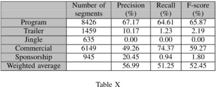
As fot the manual dataset, we provide detailed results of the CRF performance in Tables IX, X and XI. In multiple labelling of the automatic dataset, CRF provide the highest F-score in average (52.45%), even if there is a high confu-sion between labels as shown on the confuconfu-sion matrix (see Table X). Commercials and programs are the best recognized by CRFs. Other labels are difficult to be correctly labelled, especially jingles and sponsorships.
We note a high confusion between the following la-bels(see Table XI):
• jingle and commercial: More than 50% of jingles are labelled as commercials and the remainder as programs;
Number of Precision Recall F-score segments (%) (%) (%) Program 8426 67.17 64.61 65.87 Trailer 1459 10.17 1.23 2.19 Jingle 635 0.00 0.00 0.00 Commercial 6149 49.26 74.37 59.27 Sponsorship 945 20.45 0.94 1.80 Weighted average 56.99 51.25 52.45 Table X
DETAILED PERFORMANCE ON THE MULTIPLE LABELLING WITH THE
AUTOMATIC DATASET USINGCRF
Program Trailer Jingle Commercial Sponsorship Program 5444 115 8 2836 23 Trailer 562 18 0 876 4 Jingle 204 4 0 426 2 Commercial 1529 38 4 4573 6 Sponsorship 370 2 1 573 9 Table XI
MULTIPLE LABELLING OF THE AUTOMATIC DATASET USINGCRF
-CONFUSION MATRIX
• trailer and commercial: More than 50% of trailers are labelled as commercials and the remainder as programs; • sponsorship and commercial: More than 50% of spon-sorships are labelled as commercials and the remainder as programs;
• commercial and program: Almost 25% of commercials are labelled as programs and almost 30% of programs are labelled as commercials.
These results highlight the fact that the descriptors used to describe the segments are not discriminant enough to separate many successive segments.
VII. EXPLORING THE EFFICIENCY OFCRF Results obtained in the previous experiments show that CRFs are better suited to our labelling tasks than other usual machine learning techniques. In this section, two (related) issues regarding this good performance are explored. We first shed light on the importance of taking into account the sequential nature of our data, and how this is done, at different levels in CRFs. As the supervision task is tedious and costly, we then examine how CRF deal with different training set sizes, compared with the other machine learning techniques.
A. About sequentiality in CRF
Four experiments were conducted in order to shed light on the ability of CRF to take into account the sequential nature of the data. This is simply done by using different template files defining the model. Here are the different settings used for this experiment:
• CRF-all: this template indicates that the CRF uses a) information about the current observation as well as
the four before and the four next ones (corresponding to features function f(yi, xi−4, ..., xi, ..., xi+4)), and b) information about the neighbouring label, called bigram template, corresponding to feature functions
g(yi, yi−1). So, the exact formulation is:
P(y|x) = 1 Z(x)exp k1 X k=1 X i λkfk(yi, xi−4, ..., xi+4) + k2 X k=1 X i µkgk(yi−1, yi) ! (3)
• CRF-CO: here, we use a) an unigram template which considers only the current observation and its associated label (corresponding to features functionf(yi, xi)) and
b) a bigram template; so finally:
P(y|x) = 1 Z(x)exp k1 X k=1 X i λkfk(yi, xi) + k2 X k=1 X i µkgk(yi−1, yi) ! (4)
In terms of information taken into account, this formu-lation can be compared to the HMM one.
• CRF-nonB: this template is similar to CRF-all, without the bigram template.
P(y|x) = 1 Z(x)exp k1 X k=1 X i λkfk(yi, xi−4, ..., xi+4) ! (5) This formulation can be compared to the contextual setting of the standard machine learning algorithms. • CRF-CO-nonB: this last template only includes a
un-igram template which considers the current observa-tion (corresponding to features funcobserva-tion f(yi, xi)); so
finally: P(y|x) = 1 Z(x)exp k1 X k=1 X i λkfk(yi, xi) ! (6)
This formulation can be compared to thesimplesetting of the standard machine learning algorithms.
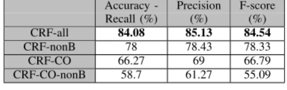
These different CRF versions are tested on the manual dataset on the multiple label task. Table XII presents the results they obtain (report to Table IV for other methods’ performance). From these experiments, one can assess the importance of the two types of sequential information taken into account in CRF. Indeed, both the label dependency and the neighbouring observations help to yield the best results. On this particular task, the latter has a greater impact
Accuracy - Precision F-score Recall (%) (%) (%) CRF-all 84.08 85.13 84.54 CRF-nonB 78 78.43 78.33 CRF-CO 66.27 69 66.79 CRF-CO-nonB 58.7 61.27 55.09 Table XII
PERFORMANCE FOR THE MULTIPLE LABELLING TASK WITH THE
MANUAL DATASET,USINGCRFAND VARIOUS CLASSIFICATION
METHODS
than the former. It is interesting to compare the results of the CRF-CO and HMM since they both exploit the same information. Yet, the CRF clearly outperforms HMM thanks to its undirected representation of the label dependency preventing any label bias problem (cf. section III-B). As expected, the CRF-nonB results yields similar results to those of thecontextualsetting of the SVM, Naive Bayes or Random Forests. Similarly, the CRF-CO-nonB, whose pre-diction only relies on the current observation, is comparable to standard machine learning techniques such as SVM, or Random Forests with the simple setting and thus also obtains similar results.
B. Training set size
As it has been said before, due to the cost of supervision, it is interesting to examine how the performance of the la-belling techniques are dependent on the training set size. For this experiment, we adopt the most difficult setting: Multiple labelling with the automatic dataset. At every learning step, we add a new sequence of segments broadcasted on the same day to the training set, learn the CRF parameters, and apply this CRF on the test set. To prevent any bias, the sequences are randomly selected, and the results are averaged over several runs. The results are shown in Figure 2.
Figure 2. Results of CRF on multiple labelling of the automatic dataset, using different sizes of the learning dataset
We note that even with a small number of sequences (3 sequences), CRF have a F-score near of its optimum. This result is interesting when compared with existing methods requiring extensive annotated data such as [4].
VIII. CONCLUSION AND FURTHER WORK
In this paper, we applied conditional random fields to the labelling of a segmented TV stream where video segments are described with robust descriptors. The TV stream was segmented with two different segmentation processes, each process leading to a specific dataset: manual and auto-matic. Our goal was to identify five kinds of broadcasts in each dataset. We obtained interesting results on the manual dataset where the precision and the recall were up to 90%. Results are lower on the automatic dataset, especially in multiple labelling where we noticed many confusions between labels. Nevertheless, CRF’s results exceed those of other classification methods such as Hidden Markov Models, which is also a probabilistic graphical model. Indeed, the CRF’s capability to handle the sequential context between video segments makes it possible to separate different kinds of programs and breaks, even when they are described with very simple features. Of course, this approach chiefly relies on the quality of the stream pre-processing steps. Dealing with the automatically segmented data is thus more challenging, especially for the multiple labelling task, which leads to high confusion between certain labels (commercial vs. jingle, commercial vs. and sponsorship...). This weakness can be explained by the over-segmentation of the automatic dataset: broadcasts are divided into many consecutive seg-ments that features are not informative enough to discrimi-nate.
Different perspectives are foreseen for this work. To im-prove our results on the multiple labelling task, especially for the automatically segmented dataset, we plan to investigate the use of content-based features, namely audio features that are specific to some kinds of breaks (for instance, there is no music and no speech into jingles). Another challenge is also to reduce the need for already labelled data in the building of the model. To achieve this goal, we plan to introduce unlabelled data and to explore the use active learning strategies to induce Conditional Random Fields.
REFERENCES
[1] X. Naturel, G. Gravier, and P. Gros, “Fast structuring of large television streams using program guides,” in4th International Workshop on Adaptive Multimedia Retrieval, AMR’06, 2006. [2] X. Naturel and P. Gros, “Detecting repeats for video structur-ing,”Multimedia Tools and Applications, vol. 38, no. 2, pp. 233–252, 2008.
[3] J.-P. Poli, “An automatic television stream structuring system for television archives holders,”Multimedia systems, vol. 38, no. 2, pp. 255–275, November 2008.
[4] G. Manson and S.-A. Berrani, “An inductive logic programming-based approach for TV stream segment clas-sification,” inIEEE International Symposium on Multimedia, ISM’08, Berkeley, Californie, USA, December 2008.
[5] A. Pranjal, R. Delip, and R. Balaraman, “Part of speech tagging and chunking with hmm and crf,” inProceedings of NLP Association of India (NLPAI) Machine Learning Contest, 2006.
[6] M. Constant, I. Tellier, D. Duchier, Y. Dupont, A. Sigogne, and S. Billot, “Int´egrer des connaissances liguistiques dans un CRF : Application `a l’apprentissage d’un segmenteur-´etiqueteur du franc¸ais,” in Traitement Automatique du Lan-gage Naturel (TALN’11), 2011.
[7] F. Sha and F. Pereira, “Shallow parsing with conditional random fields,” in Proceedings of the 2003 Conference of the North American Chapter of the Association for Computa-tional Linguistics on Human Language Technology - Volume 1, ser. NAACL ’03, 2003.
[8] T. Wang, J. Li, Q. Diao, Y. Z. Wei Hu, and C. Dulong, “Semantic event detection using conditional random fields,” inIEEE Conference on Computer Vision and Pattern Recog-nition Workshop (CVPRW ’06), 2006.
[9] N. Zhang, L.-Y. Duan, Q. Huang, L. Li, W. Gao, and L. Guan, “Automatic video genre categorization and event detection techniques on large-scale sports data,” in Conference of the Center for Advanced Studies on Collaborative Research (CASCON’10), 2010.
[10] W.-L. Lu, J.-A. Ting, K. P. Murphy, and J. J. Little, “Iden-tifying players in broadcast sports videos using conditional random fields,” inIEEE Conference on Computer Vision and Pattern Recognition (CVPR ’11), 2011.
[11] L. R. Rabiner and B. H. Juang, “An introduction to hidden Markov models,” inIEEE ASSP Magazine, 1986.
[12] L. R. Rabiner, “A tutorial on Hidden Markov Models and selected applications in speech recognition,” inProceedings of the IEEE, 1989, pp. 257–286.
[13] J. Lafferty, A. McCallum, and F. Pereira, “Conditional ran-dom fields: Probabilistic models for segmenting and labeling sequence data,” in International Conference on Machine Learning (ICML), 2001.
[14] S. Della Pietra, V. Della Pietra, and J. Lafferty, “Inducing features of random fields,” IEEE Transactions on Pattern Analysis and Machine Intelligence, vol. 19, no. 4, pp. 380– 393, 1997.
[15] N. N. Schraudolph, J. Yu, and S. G¨unter, “A stochastic quasi-Newton method for online convex optimization,” in Proceedings of 11th International Conference on Artificial Intelligence and Statistics, ser. Workshop and Conference Proceedings, vol. 2, San Juan, Puerto Rico, 2007, pp. 436– 443.
[16] Z. A. A. Ibrahim and P. Gros, “TV stream structuring,”ISRN Journal on Signal Processing, vol. 2011, no. 1, April 2011.