UC Riverside Previously Published Works
Title
FreePSI: an alignment-free approach to estimating exon-inclusion ratios without a reference
transcriptome.
Permalink
https://escholarship.org/uc/item/3r6456j6
Journal
Nucleic acids research, 46(2)
ISSN
0305-1048
Authors
Zhou, Jianyu
Ma, Shining
Wang, Dongfang
et al.
Publication Date
2018
DOI
10.1093/nar/gkx1059
Peer reviewed
eScholarship.org
Powered by the California Digital Library
FreePSI: an alignment-free approach to estimating
exon-inclusion ratios without a reference
transcriptome
Jianyu Zhou
1,2, Shining Ma
3, Dongfang Wang
1, Jianyang Zeng
4and Tao Jiang
1,2,5,*1MOE Key Laboratory of Bioinformatics; Bioinformatics Division and Center for Synthetic & Systems Biology, TNLIST,
Tsinghua University, Beijing 100084, China,2Department of Computer Science and Technology, Tsinghua University, Beijing 100084, China,3Department of Statistics, Stanford University, Stanford, CA 94305, USA,4Institute for
Interdisciplinary Information Sciences, Tsinghua University, Beijing 100084, China and5Department of Computer Science and Engineering, University of California, Riverside, CA 92521, USA
Received May 17, 2017; Revised October 11, 2017; Editorial Decision October 16, 2017; Accepted October 19, 2017
ABSTRACT
Alternative splicing plays an important role in many cellular processes of eukaryotic organisms. The exon-inclusion ratio, also known as percent spliced in, is often regarded as one of the most effective measures of alternative splicing events. The exist-ing methods for estimatexist-ing exon-inclusion ratios at the genome scale all require the existence of a ref-erence transcriptome. In this paper, we propose an alignment-free method, FreePSI, to perform genome-wide estimation of exon-inclusion ratios from RNA-Seq data without relying on the guidance of a ref-erence transcriptome. It uses a novel probabilistic generative model based on k-mer profiles to quan-tify the exon-inclusion ratios at the genome scale and an efficient expectation-maximization algorithm based on a divide-and-conquer strategy and ultra-fast conjugate gradient projection descent method to solve the model. We compare FreePSI with the ex-isting methods on simulated and real RNA-seq data in terms of both accuracy and efficiency and show that it is able to achieve very good performance even though a reference transcriptome is not provided. Our results suggest that FreePSI may have impor-tant applications in performing alternative splicing analysis for organisms that do not have quality refer-ence transcriptomes. FreePSI is implemented inC++
and freely available to the public on GitHub. INTRODUCTION
Alternative splicing plays a crucial role in many cellular pro-cesses of eukaryotic organisms (1). It allows a gene to be transcribed into multiple isoforms (or mRNA transcripts)
and hence increases the phenotypic complexity of an or-ganism without increasing its genetic complexity. The exon-inclusion ratio, also known as percent spliced in (PSI), is a popular statistic for measuring alternative splicing events (2). It is defined as the ratio of the relative abundance of all isoforms containing a certain exon over the relative abun-dance of all isoforms of the gene containing the exon. In other words, the PSI value of an exon tells us how often the exon occurs in all the isoforms of the gene that contains the exon. The PSI values of a gene reflect the intensity of its alternative splicing events and have been widely used in dif-ferential expression analysis that aims at detecting spliced exons (3) as well as in the exploration of biological mecha-nisms of alternative splicing (4–6).
A genome-wide estimation of PSI values remains difficult until the advent of high-throughput RNA-seq technology (7). In recent years, many computational methods have been proposed to analyze RNA-seq data (8), including several for performing genome-wide PSI estimation. The methods for PSI analysis generally fall into two categories: isoform-centric or exon-isoform-centric (9). An isoform-centric PSI analysis (10) begins by estimating the relative abundance of each iso-form by using a quantification tool such as Cufflinks (11), RSEM (12) CEM (13) or eXpress (14) if a reference tran-scriptome is given. Once the relative abundance levels of all isoforms have been quantified, the PSI values of each exon in the genome can be easily derived. If no reference tran-scriptome is available, a trantran-scriptome assembly tool such as Cufflinks, IsoLasso (15), StringTie (16) or TransComb (17) can be used to infer the expressed isoforms as well as their relative abundance from the input RNA-seq data and reference genome.
A common feature of the above quantification/assembly methods is that they all require the input RNA-seq reads to be mapped (or aligned) to the reference genome (or tran-scriptome) as a preprocessing step. This can be achieved by
*To whom correspondence should be addressed. Tel: +1 951 8272991; Fax: +1 951 8274643; Email: [email protected]
C
The Author(s) 2017. Published by Oxford University Press on behalf of Nucleic Acids Research.
This is an Open Access article distributed under the terms of the Creative Commons Attribution License (http://creativecommons.org/licenses/by-nc/4.0/), which permits non-commercial re-use, distribution, and reproduction in any medium, provided the original work is properly cited. For commercial re-use, please contact [email protected]
using alignment tools such as Bowtie (18), TopHat (19,20) and HISAT (21). On the other hand, an alignment-free ap-proach for abundance quantification has been proposed re-cently and implemented in Sailfish (22). The method uses
k-mer counts to construct profiles of both the input RNA-seq reads and reference transcriptome, and a probabilis-tic generative model based on the profiles to estimate the abundance of each isoform. As reported in (22), Sailfish is able to achieve a comparable overall accuracy as Cufflinks while maintaining a much higher efficiency. The high effi-ciency of Sailfish is helped by a light-weight expectation-maximization algorithm for solving the probabilistic model and the parallelizablek-mer counting method evolved from Jellyfish (23). Inspired by the alignment-free approach, some ‘pseudo-alignment’ (or ‘quasi-mapping’) based meth-ods including Kallisto (24) and Salmon (25) have been pro-posed very recently in the literature with further improved performance. These methods do not attempt to map reads to precise locations of the reference genome. Instead, they try to identify all isoforms in the reference transcriptome that may potentially contain each specific read. Note that the alignment-free or pseudo-alignment-based approaches for isoform abundance quantification require the existence of a reference transcriptome and their performance clearly depends on the quality of the reference transcriptome.
Exon-centric methods including MISO (26), MATS (27) and rMATS (28) focus on specific exons instead of an en-tire exome and analyze alternative splicing events such as exon skipping, mutually exclusive exons, intron retention as well as alternative (5 or 3) boundaries based on the PSI values of the exons. In particular, MISO can perform alter-native splicing analysis on a single biological sample or dif-ferential expression analysis on two samples, while MATS and rMATS specialize in the comparison of two samples. These methods all require mapped RNA-seq reads and use Bayesian inference to perform PSI estimation that incurs significant running time. Moreover, the alternative splicing events to be analyzed have to be provided by the user in ad-vance or extracted from a reference transcriptome.
Clearly, the availability of a high quality reference tran-scriptome is critical for both isoform-centric and exon-centric PSI estimation methods. Although transcriptomes can be assembled from RNA-seq data on-the-fly by using assembly tools such as Cufflinks, IsoLasso, StringTie or TransComb, they are likely to contain a high degree of noise (9). Such noise may significantly affect the accuracy of sub-sequent PSI estimation. Moreover, even if a reference tran-scriptome is available, it may not cover all expressed iso-forms in the input RNA-seq data. Such an incomplete ref-erence transcriptome may also misguide subsequent PSI es-timation.
In this paper, we propose a new method for genome-wide PSI estimation, called FreePSI, that requires neither a reference transcriptome (hence, transcriptome-free) nor the mapping of RNA-seq reads (hence, alignment-free). The first freedom allows FreePSI to work effectively when a high quality reference transcriptome is unavailable and the sec-ond freedom not only helps make FreePSI more efficient, it also eliminates the necessity of dealing with multi-reads, which is a challenging problem by itself. Note that this is the first alignment-free method in RNA-seq data analysis
that does not require a reference transcriptome. An outline of the method is given below.
FreePSI takes as the input a reference genome with exon boundary annotation and a set of RNA-seq reads. Since a reference transcriptome is not assumed, it uses a weighted directed bipartite graph (called an abundance flow graph) to represent all possible isoforms of a gene and their ex-pression levels. In such a graph, each vertex represents an exon boundary and each edge represents either an exon or an exon junction. The weight of an edge represents the to-tal relative abundance of all isoforms covering the corre-sponding exon or junction. Obviously, to estimate the PSI value of each exon, it suffices to infer the edge weights in every abundance flow graph. By regarding each edge as a sequence ofk-mers, FreePSI constructs a novel probabilis-tic model for generating all observed k-mers in the input RNA-seq reads based on the abundance flow graphs for all genes. It then employs the expectation-maximization (EM) framework to solve a genome-wide maximum likelihood es-timation (MLE) of the model and a divide-and-conquer strategy to factorize the key optimization problem in the M-step into independent subproblems for each gene, which are then solved by an ultrafast algorithm, conjugate gradi-ent projection descgradi-ent. The above factorization is crucial for the efficiency of FreePSI because unlike Sailfish whose EM algorithm involves an M-step with a closed-form solution due to the given reference transcriptome, the key optimiza-tion problem in the M-step of the EM algorithm of FreePSI does not have a closed-form solution. Finally, it uses a post-processing procedure based on straightforward correlation analysis to “smooth out” the PSI values in each gene.
To evaluate the performance of FreePSI, we compare it with isoform-centric methods including Salmon (the most recent isoform abundance quantification method) and Cuf-flinks (the most popular transcriptome assembly and iso-form quantification method) as well as a representative exon-centric method MISO on both simulated and real data. Our experimental results demonstrate that although FreePSI is unable to match the overall performance of Salmon on simulated data where the correct reference tran-scriptome is provided, it performs better than Cufflinks without assuming a reference transcriptome (denoted as Cufflinks-A) and MISO in terms of both accuracy and ef-ficiency. In particular, for genes that have large proportions of multi-mapped reads, FreePSI achieves significantly bet-ter accuracy than Cufflinks-A. On the other hand, on a real dataset where the true reference transcriptome is un-known, both FreePSI and Cufflinks-A are able to outper-form Salmon significantly in terms of accuracy. These re-sults suggest that FreePSI may have important applications in alternative splicing analysis when a high quality reference transcriptome is unavailable.
MATERIALS AND METHODS
Overview
As outlined in Introduction, FreePSI estimates the PSI values of all annotated exons on the reference genome from RNA-seq reads and is both transcriptome-free and alignment-free. It uses a weighted directed bipartite graph, called an abundance flow graph, to represent all possible
A
B
C D
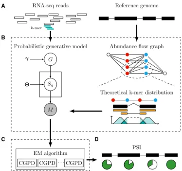
Figure 1. An overview of FreePSI. (A) The input of FreePSI includes a reference genome with exon boundary annotation and a set of RNA-seq reads. (B) The main component of FreePSI is a probabilistic generative model. The abundance flow graph represents all possible isoforms and their abundance levels. For each exon (or junction), the (theoretical) dis-tribution ofk-mers in the exon (or junction, respectively) is derived by as-suming that the reads were uniformly sequenced. (C) An EM algorithm is employed to perform genome-wide inference for the model, and a divided-and-conquer strategy decomposes the key optimization problem in the M-step into independent subproblems for each gene. Each subproblem is solved using a conjugate gradient projection algorithm. (D) The output of FreePSI includes estimated PSI values for all exons.
isoforms of a gene and their abundance levels. The PSI val-ues of all exons in the gene can be easily derived from the weights of the edges in the graph, where each edge repre-sents an exon or junction in all possible isoforms. The edge weights are constrained by linear inequalities and can be estimated via an free approach. The alignment-free estimation formulates (theoretical)k-mer distributions on exons/junctions by assuming that the reads were uni-formly sequenced and uses a novel probabilistic generative model to describe all observed k-mers in the reads. Then it computes a genome-wide MLE of the model by the EM framework, and uses a divided-and-conquer strategy to de-compose the key optimization problem in the M-step into independent constrained nonlinear optimization subprob-lems for each gene. These subprobsubprob-lems are solved in par-allel by using an elaborate implementation of an ultrafast conjugate gradient projection descent algorithm. Figure 1
illustrates a flowchart of FreePSI. The details of FreePSI are given in the following subsections.
Abundance flow graph
Anabundance flow graph(AFG) represents all possible iso-forms of a gene and their relative abundance based on the concept ofsegments. There are two types of segments: exon segments and junction segments. An exon segment is de-fined as an interval on the reference genome sandwiched
between two consecutive exon boundaries. For any pair of exon segmentsiand jthat can potentially be joined by a junction read, a junction segment is defined as the con-catenation of the lengthLread−1 suffix ofiand the length Lread−1 prefix ofj, whereLread represents the read length. Note that exon segments and junction segments are referred to as expressed segments and junctions, respectively, in (15). Letαh denote the relative abundance of isoformhandαij
denote the total relative abundance of all isoforms cover-ing the junction segment formed by exon segmentsiandj. For convenience, we use the notationαiito denote the total
relative abundance of all isoforms covering exon segmenti. The PSI value of exon segmentican be calculated by the following equation: ψi = αi i h αh
Figure2A illustrates an example of segments. Supplemen-tary Section S1.1 gives the formal definitions ofαand PSI as well as a detailed derivation of the above equation.
An AFG is essentially a weighted directed bipartite graph (U,V,E). Here,U={ui|1≤i≤nexon}represents the left
part of the vertices, where ui denotes the starting
bound-ary of exon segment iand nexon the number of exon
seg-ments, andV={vi|1≤i≤nexon}represents the right part,
wherevi denotes the ending boundary of exon segmenti.
The edges are separated into the forward edges and back-ward edges, denoted asE=(E→,E←). The forward edges,
E→={<ui,vi>|1≤i≤nexon}, represent the exon segments
and are weighted asαii. The backward edges,E← ={<vi,
uj>|1≤i<j≤nexon}, represent the junction segments and
are weighted asαij. In addition, two verticessandt
repre-senting dummy (source and sink) exons are introduced in the graph to accommodate isoforms with alternative tran-scription start sites and/or polyadenylation cleavage sites. For each i, an edge <s, ui>is added with weight αsi to
denote the total relative abundance of all isoforms start-ing with exon segmentiand an edge<vi,t>is added with
weightαitto denote the total relative abundance of all
iso-forms ending with exon segmenti. An example AFG for a gene consisting of four exon segments is shown in Fig-ure2B. Note that although an AFG looks very similar to asplicing graphintroduced in (29), its edges represent exon and junction segments rather than exons and introns.
Clearly, every isoform of the gene corresponds to a path in the AFG fromsto t, and vice versa. Hence, the total relative abundance of all isoforms of the gene is equal to the summation of allαsi. Moreover, the edge weights in the
AFG should satisfy the “flow conservation” property. In other words, for each vertex inU∪V, the total weight of all its in-edges is equal to the total weight of all its out-edges. Supplementary Figure S1 provides an example of the flow conservation property. Using this property, the PSI value of an exon segment can be expressed as
ψi = αi i i α i i− i j>iα i j (1)
A
B
D
C
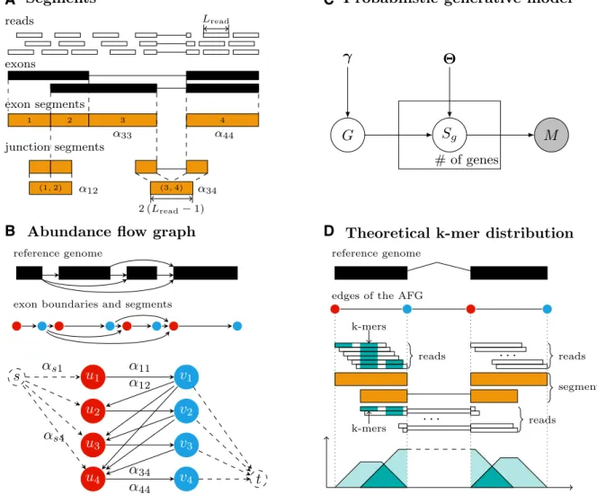
Figure 2. (A) Segments. Every annotated exon (black bar) corresponds to one or more exon segments and has two boundaries. If the annotated exons from different isoforms overlap, they are partitioned into disjoint exon segments. If exon segmentiis joined with exon segmentjin an isoform, a junction segment of length 2(Lread−1) would be formed. For examples, the junction segment (1, 2) is formed by exon segments 1 and 2 and the junction segment (3,
4) by exon segments 3 and 4. The parameterαassociated with each segment represents the total relative abundance of all isoforms covering the segment. (B) Abundance flow graph. The figure shows an example AFG for a gene consisting of four exon segments. The AFG is constructed according to the exon boundary annotation of the reference genome. The red vertices represent the starting boundaries of the exon segments, and the blue vertices represent the ending boundaries of the exon segments. The forward edges from the red vertices to the blue vertices represent the exon segments and the backward edges from the blue vertices to the red vertices represent the junction segments. The parameterαdefined for each segment is assigned as its corresponding edge weight. Two dummy verticessandtare introduced to handle isoforms that begin and/or end with different exon segments. (C) Probabilistic generative model. The graphical structure of the probabilistic generative model is a three-layer Bayesian network. The distributions of the random variablesGandSg
are determined by the parametersγand.Sghas gene number replicates, and the random variableMis observable. (D) Theoreticalk-mer distribution.
The theoretical distribution ofk-mers is derived from the assumption that the reads are uniformly distributed in an isoform. Since each read belongs to one segment, they are also uniformly distributed in a segment. Hence,k-mers near the middle of a segment are usually covered by more reads in the segment thank-mers near the boundaries of the segment. This gives rise to a trapezoid shaped theoretical distribution ofk-mers in a segment. Note that ak-mer may be shared by multiple (exon and junction) segments.
The following inequalities will help us in the estimation of theαvalues: αi i ≥ j<i αj i, αi i ≥ j>i αi j (2)
The detailed derivations of these linear constraints are given in Supplementary Section S1.2.
Probabilistic generative model
Since each read is generated from a segment randomly and each read defines a set ofk-mers, each segment generates a
random set ofk-mers. We construct a three-layer Bayesian network to model the mixture of allk-mers generated by the segments from all genes, as shown in Figure2C. In the following,sdenotes a segment (exon or junction) and ga gene. LetGrepresent a random gene,Sga random segment
of geneg, for eachg, andMa randomk-mer. We use P(G
=g)=γg to represent the probability that a read is
gen-erated from geneg, P(Sg=s|G=g)=θgsto represent the
conditional probability that a read generated from geneg
belongs to segments, and P(M=m) to denote the prob-ability of observingk-merm. Then, the probability of an
observedk-mermcan be expressed as P (M=m)= g γg s∈g θgsP M=m|Sg=s,G=g
where P(M=m|Sg=s,G=g) denotes the (theoretical)
dis-tribution ofk-mers on segmentsin genegassuming that the reads are sampled uniformly. See Supplementary Sec-tion S2.3 for a detailed derivaSec-tion of this probability.
Again assuming that the reads are uniformly distributed on each segment, then the parameters α can be approxi-mated by γ and θ as follows, if the relative abundance is measured by TPM (transcripts per million) :
αgs ≈ Z2 Z1 γgθgs Lgs (3) where αgs denotes the total relative abundance of all
iso-forms covering segmentsin geneg,Z1andZ2are
normal-ization constants, andLgsis the effective length of segment
sin geneg. That is, ifLgs denotes the length of segments
in geneg, thenLgs=Lgs−Lread+1. Hence, the PSI value
defined in Equation1can be estimated fromθand the linear constraints in Equation2can also be applied toθ. The de-tailed derivation of the above approximation can be found in Supplementary Section S2.4.
The theoreticalk-mer distribution over a segment is nec-essary because even if the reads are sampled uniformly, the
k-mers are not distributed uniformly across the segment. See Figure2D for an illustration. Note that the segment de-finesLgsdistinct reads, and each read containsLread−K+1
k-mers. LetFgsmdenote the number of distinct reads
cover-ing ak-mermon segmentsin geneg. Then, the theoretical distribution of allk-mers generated from the segment can be written as PM=m|Sg=s,G=g = Fgsm Lgs(Lread−K+1) (4) From now on, letcgsmdenote P(M=m|Sg=s,G=g). More
details of the above discussion are given in Supplementary Section S2.5.
Therefore, to quantify PSI values, it suffices to perform a MLE of the parametersγandθ.
Expectation-maximization algorithm
The MLE can be formulated as the following nonlinear con-strained optimization problem:
max m nmlog g γg s∈g θgscgsm
s.t. Agθg ≥0, for all genesg
s∈g
θgs=1, for all genesg
g
γg =1, ∀γg ≥0, ∀θgs≥0
wherenmdenotes the number of occurrences ofk-mermin
all input reads,θg the vector formed by allθgs,s∈g, and
Agθgthe matrix form of the linear constraints in Equation
(2) (see Supplementary Equations S2.7–S2.10 for details). See Supplementary Section S3.1 for this formulation. We develop an EM algorithm below to solve the optimization problem iteratively.
Letγdenote the vector formed by allγgandthe matrix
formed by stacking all vectorsθg. Before the iteration starts,
an initial feasible solutionγ(0)and(0)is obtained based on
thek-mer profiles of the input RNA-seq reads, as sketched in Algorithm S1 of Supplementary Section S3.2. In general, the E-step of the EM algorithm is to generate a function for the expected log-likelihood based on the current estima-tion of the parameters. Assuming thattiterations have been completed, the expected log-likelihood is then
Q(γ,)=QI(γ)+ g QII g θg where QI(γ)= m g μ(t) gmlog γg QII g θg = m μ(t) gmlog s∈g θgscgsm μ(t) gm = γ(t) g s∈gθ (t) gscgsm g γ (t) g s∈gθ (t) gscgsm
whereμ(gmt) denotes the posterior probability ofk-merm
be-ing generated from genegbased on the last estimations of
γ(t) and (t). More details of the derivation are given in
Supplementary Section S3.2. The expectation Q(γ,) is decomposed into the summation of two terms,QI(γ) and
gQIIg
θg
, that involve independent parameters and con-straints.
The M-step is to maximize the expected log-likelihood given in the E-step. Given the above decomposition, the maximization problem can be divided into two parts. The first part is
max QI(γ) s.t.
g
γg =1, ∀γg≥0
This part has a closed-form solution (see Supplementary Section S3.2). The second partgQII
g
θg
can be solved by a divide-and-conquer strategy, which leads to an opti-mization subproblem for each geneg:
max QIIg θg s.t. Agθg≥0, s∈g θgs=1, ∀θgs≥0
Unfortunately, these subproblems do not have closed-form solutions due to the presence of linear inequality con-straints. Hence, we use a conjugate gradient projection de-scent algorithm to solve them.
The conjugate gradient projection descent (CGPD) algo-rithm (30) is an efficient algorithm for convex optimization under linear constraints. The detailed CGPD algorithm is given in Algorithm S2 of Supplementary Section S3.3. Its key idea is to perform line search along the conjugate direc-tions in the null space of active constraints. Since the ob-jective functionQII
g
θg
in our problem is a continuous dif-ferentiable convex function and all the constraints are lin-ear, the CGPD algorithm is particularly suitable. Because
∇QII
g
θg
is much easier to compute thanQII
g
θg
(Sup-plementary Section S4.2.1), we choose the secant method for line search in CGPD, which only requires the first-order derivatives of the objective function and has a super linear convergence rate.
Post-processing
The above EM algorithm results in an estimation of the parametersγ and. Since these parameters only provide an approximation of the parametersα (and thus PSI), as shown in equation3, some post-processing could be applied to refine the raw estimation of PSI values. We adopt a post-processing procedure based on two assumptions: for each gene, (i) a small number of isoforms are expressed and (ii) there exists an exon segment included in all expressed iso-form.
The first assumption implies that the PSI values of the exon segments from each gene should fall into a small set of distinct numbers. Hence, we could potentially reduce noise by clustering similar PSI values. An average-linkage hierarchical clustering algorithm with Euclidean distance is adopted here. Once a hierarchical clustering tree is ob-tained, we cut it to result in the least number of clusters such that either the maximum standard deviation of PSI values in each cluster is less than 0.06 or the mean of the standard de-viations of PSI values in all clusters is less than 0.05. Then, the raw estimates of PSI values in each cluster are revised to the mean values of the cluster.
The second assumption implies that there should be at least one exon segment with PSI value equal to 100% PSI. Hence, we rescale the above revised PSI values by dividing each by the maximum PSI value of any exon segment in the same gene.
It turns out that both the linear constraints in Equation
2and the above processing steps are crucial for FreePSI to obtain a good estimation of exon-inclusion ratios.
Implementation
FreePSI is implemented mainly inC++. We utilize the third-part library Eigenfor matrix manipulations. Paralleliza-tion of the program is achieved by usingOpenMP. Some key issues of the implementation are discussed below.
K-mer hash table. As a preprocessing step, Jellyfish is in-voked to countk-mers in the input RNA-seq reads. Then, FreePSI indexes eachk-mer as a 64-bit integer using a linear algorithm that scans the reads and segments only once, as shown in Algorithm S3 of Supplementary Section S4.1. The
k-mer indices are then hashed into aC++11built-in hash ta-ble,unordered map. Each entry of the hash table stores
two pieces of information: one is the count of thek-mer in the reads and the other is a list of segments containing the
k-mer as well as the corresponding coefficientcgsm. During
hashing, allk-mers that share the same segments are com-bined into one representativek-mer, and their counts and the coefficients are also combined. This shrinks the size of the hash table significantly. In our simulation experiments, the shrinkage rates were∼80% on average, which greatly re-duced the computational complexity of subsequent steps. A similar strategy was also adopted in (22).
Implementation of the EM algorithm. The convergence cri-terion of the EM algorithm is that the log-likelihood in-creases by less than 10−6in an iteration. In order to speed
up the computation, sparse matrix and parallelization tech-niques are adopted. In particular, thereductionfunction inOpenMPis employed to allow for concurrent calculation of the summation in the E-step of the algorithm. On the other hand, the M-step, composed of many independent subproblems, can be easily parallelized withOpenMP.
Efficiency improvements for CGPD. The CGPD algorithm used in the M-step is the efficiency bottleneck of FreePSI. Four techniques are implemented to improve its efficiency.
The first one is reordering matrix multiplications, which has also been considered carefully in all implementations of the CGPD algorithm. It is well-known that rearranging the order of matrix multiplications can potentially reduce time complexity drastically. In particular, the matrix multi-plications in CGPD can be reordered so that only matrix-vector multiplications are performed. In our simulation ex-periments, we found that this technique contributed signif-icantly to the efficiency of FreePSI.
The second strategy is the compaction of sparse param-eters. Before calling CGPD, the zero entries inθgas well as
their associatedcgsm’s and optimization constraints are
re-moved. Only the remaining parameters are updated by the CGPD algorithm. The compaction may reduce the number of iterations by lowering the dimensionality of the search space in CGPD.
The third technique is offline computation for a part of
∇QII g θg . The gradient∇QII g θg
is required in every iter-ation of CGPD. We observe that the gradient can be de-composed into the product of an iteration-invariant part and an iteration-variant part, while the iteration-invariant part consumes a large amount of running time (see Sup-plementary Section S4.2.1 for the details). So, computing the iteration-invariant part in advance can surely enhance FreePSI’s efficiency.
The last technique is replacing outer products of vec-tors into in-space column-wise operations. The CGPD al-gorithm computes outer products of vectors during its itera-tions. A direct implementation allocates new memory space for storing the result matrix of each outer product, which is then added to or subtracted from another matrix. However, the storage of intermediate matrices is unnecessary. Hence, we replace an outer product operation by some column-wise operations that can be performed in-space. That is, the col-umn vector is first multiplied with an element of the row vector. The result is then added to or subtracted from the
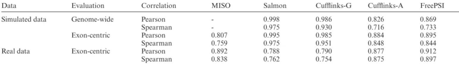
Table 1. Accuracy measured by both Pearson and Spearman correlations of the methods on both simulated and real RNA-seq datasets
Data Evaluation Correlation MISO Salmon Cufflinks-G Cufflinks-A FreePSI
Simulated data Genome-wide Pearson - 0.998 0.986 0.826 0.869
Spearman - 0.975 0.930 0.716 0.733
Exon-centric Pearson 0.807 0.995 0.985 0.884 0.895
Spearman 0.759 0.975 0.951 0.848 0.844
Real data Exon-centric Pearson 0.892 0.788 0.790 0.877 0.912
Spearman 0.838 0.762 0.754 0.875 0.897
corresponding column of another matrix (see Supplemen-tary Section S4.2.2 for more details).
RESULTS
In this section, we evaluate the performance of FreePSI by comparing it with the other state-of-the-art PSI quan-tification methods on both simulated and real RNA-seq data. More specifically, we compare two transcriptome-free methods including FreePSI and Cufflinks (v2.2.1) and three transcriptome-guided methods including Salmon (v0.7.2), Cufflinks (v2.2.1) and MISO (v0.5.3). Here, Cufflinks is considered as both a transcriptome-free method and a transcriptome-guided method. In the former case (denoted as Cufflinks-A), it is used to perform both transcriptome assembly and abundance quantification; but in the latter case (denoted as Cufflinks-G), it is only run to quantify the relative abundance of the annotated isoforms. In addition, HISAT (v2.0.4) is used for mapping reads in the alignment-based methods (Cufflinks and MISO) and Jellyfish (v2.2.6) is used for countingk-mers in FreePSI. All the methods are run on a 64-bit Linux server consisting of two CPUs with 16 cores each and 96 GB memory.
Performance on simulated data
We use Flux Simulator (31) to simulate RNA-seq data. Here, UCSChg38is used as the reference genome and the RefSeq refGene annotation (23,983 genes and 57,822 iso-forms) is used as the reference transcriptome. The expres-sion level of each isoform is assigned according to a power-law distribution, and roughly 100 million strand-specific paired-end reads of length 76bp are simulated with the de-fault sequencing error profile. The overall mapping rate of the simulated reads to the reference genome is 92.2%.
FreePSI requires annotated exon boundaries as a part of its input. Although such information is provided in the reference genome (UCSChg38), in order to be consistent with the simulation, we extract exon boundaries from the reference transcriptome by merging the annotated isoforms (since the reads are simulated from them directly). In partic-ular, overlapping exons from different isoforms are split into disjoint “short exons”, and all short exons of lengths>30 bp are retained in the exon annotation. To avoid dealing with genes with too many short exons, genes with more than 40 short exons are removed from the annotation, which ac-counts for 1.4% of all genes. Finally, the exon annotation is represented as a series of disjoint intervals on the refer-ence genome. The annotation of alternative splicing events required by MISO is extracted from the reference transcrip-tome using a built-in toolkit of MISO. It includes five types
of alternative splicing events: skipped exon, retained intron, mutually exclusive exons and alternative (5and 3) bound-aries.
Thek-mer length is a key parameter in FreePSI. It is set as 27 bp in the experiment. (See Supplementary Section S5.4 for a discussion on the impact of thek-mer length on the performance of FreePSI.) Jellyfish is used to count 27-mers from the simulated RNA-seq reads while filtering out k -mers that contain any base with error probability over 1%. Both Cufflinks-A and Cufflinks-G are run with the “rescue method” for multi-read refinement and the positional bias correction enabled, while MISO and Salmon are run with the default configurations. More details of the running con-figurations are given in Supplementary Section S6.
To obtain the ground truth for evaluation, we transform the simulated expression levels of the annotated isoforms into PSI values of each annotated exon. The accuracy per-formance is evaluated in two ways: genome-wide and exon-centric. The genome-wide evaluation tests the overall accu-racy of estimated PSI values across all exons of all genes. MISO is excluded from this evaluation because it does not provide a genome-wide estimation of PSI values. Totally, 7032 genes with expression levels over 10 TPM are selected for the evaluation. The accuracy is measured by the Pear-son and Spearman correlations between estimated and true PSI values of all annotated exons in the selected genes. The results of the compared methods are listed in Table1(rows 1 and 2).
The exon-centric evaluation is concerned with the accu-racy of estimated PSI values of alternatively spliced exons, which are exons with over 95% of their regions covered by the annotated alternative splicing events extracted above. According to this definition, 10,919 alternatively spliced ex-ons are selected for the evaluation. The Pearson and Spear-man correlation coefficients between estimated and true PSI values of alternatively spliced exons are listed in Table 1
(rows 3 and 4).
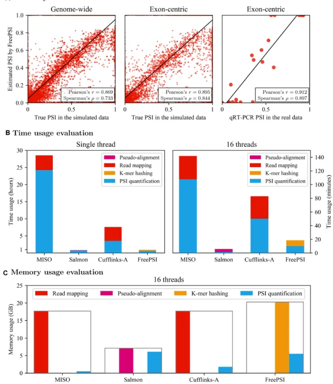
Both genome-wide and exon-centric evaluations arrive at similar conclusions. The transcriptome-guided isoform-centric methods, Salmon and Cufflinks-G, delivered nearly perfect estimates of PSI. This is clearly due to the fact that the methods used the same reference transcriptome as em-ployed in the simulation. On the other hand, the accuracy of the exon-centric method, MISO, is just acceptable. The transcriptome-free methods, FreePSI and Cufflinks-A, were also able to deliver strong correlation results, with FreePSI performing slightly better than Cufflinks-A. A scatter plot of the estimation results of FreePSI is shown in Figure3A. Similar scatter plots for the other methods can be found in Figures S2 and S3 of Supplementary Section S5.1.
Figure 3. (A) Accuracy of FreePSI. The left and center scatter plots show the correlation between the true PSI values and PSI values estimated by FreePSI on the simulated data using genome-wide and exon-centric evaluation methods, respectively. The right scatter plot shows the result of FreePSI on the real data. The Y-axis in these plots represents the estimated values of PSI and the X-axis the ground truth, respectively. (B) Time usage evaluation. The left histogram shows the time usages in hours of different methods with a single thread, while the right histogram shows the time usages in minutes of the methods with 16 threads. Color is used to break the running time of a method into preprocessing time and quantification time. (C) Memory usage evaluation. This histogram shows the memory usages in GB of different methods with 16 threads. Color is used to break the memory usage of a method into preprocessing memory and quantification memory. The frame boxing the bars represents the peak memory usage of each method.
Performance on real data
Although experiments on real data can provide a more real-istic assessment of performance, ground truth is often diffi-cult to obtain for real data. In the evaluation of many RNA-seq quantification methods on real data, the results of quan-titative real-time polymerase chain reaction (qRT-PCR) ex-periments have been used as the ground truth of expression levels of isoforms/genes. The limited number of isoforms or splicing events considered in qRT-PCR experiments makes it difficult to perform a genome-wide evaluation, but we can still use it to conduct an exon-centric evaluation of the PSI estimation methods.
We download the qRT-PCR data together with RNA-seq data studied in (28) (SRA accession: SRR536348). The RNA-seq dataset consists of ∼250 million strand-specific paired-end reads with length 101 bp. The qRT-PCR data concern 34 skipped exon events under the UCSChg19 an-notation, and provide the true PSI values of these events. To process the RNA-seq data, we first use Sickle (32) (https: //github.com/najoshi/sickle) to perform quality control on the reads. Then, the tolerated error probability in Jellyfish is decreased to 0.1% for each base when it is used to count
k-mers.k-mers that occur fewer than 10 times are removed. The other processing steps are identical to those in the sim-ulation experiment.
Out of the 34 skipped exons detected by the qRT-PCR data, 22 can be mapped to our annotated exon boundaries. Hence, we perform an exon-centric evaluation only on these 22 skipped exons. The Pearson and Spearman correlation coefficients between qRT-PCR and estimated PSI values es-timated by different methods on these 22 exons are listed in Table1(rows 5 and 6).
We observe that the transcriptome-guided methods Salmon and Cufflinks-G performed much worse than the other methods on this real dataset. This is perhaps due to the difference between the reference transcriptome and the true transcriptome expressed in the real data. In particular, Salmon and Cufflinks-G only estimated the relative abun-dance for the annotated isoforms, and would ignore all iso-forms that are actually expressed in the data but missing in the reference transcriptome. Such reliance on a correct ref-erence transcriptome might explain the 20% accuracy per-formance drop on real data compared with the simulation experiment. On the other hand, MISO performed much bet-ter on this real data than on the simulated data. The good performance of MISO on these 22 splicing events can per-haps be explained by the fact that it is designed for estimat-ing PSI values of specific splicestimat-ing events. The transcriptome-free methods, FreePSI and Cufflinks-A, continued to de-liver strong correlation coefficients, again with FreePSI per-forming better than Cufflinks-A. Since these methods do not rely a given reference transcriptome, they are able to deal with any set of expressed isoforms and provide robust performance on data with unknown (or incomplete) tran-scriptomes. A scatter plot of the results of FreePSI is shown in Figure 3A, and scatter plots for the other methods are given in Supplementary Figrue S4 of Supplementary Sec-tion S5.2.
Efficiency evaluation
The efficiency of a quantification method is as impor-tant as its accuracy. We present the running time of the above PSI quantification methods using a single thread or 16 threads separately in the above simulation experi-ment. While single-thread running time represents the se-quential time-efficiency of an algorithm, 16-thread run-ning time could suggest the parallelizability of the algo-rithm as well as its practical time efficiency when computer clusters (or multi-core machines) are available. Since the methods preprocess data differently, we also show the time spent on preprocessing in each method besides quantifi-cation. In particular, the alignment-based methods (Cuf-flinks and MISO) begin by mapping reads to the reference genome using HISAT, the pseudo-alignment-based method (Salmon) starts by constructing a pseudo-alignment and the alignment-free method (FreePSI) begins by building thek -mer hash table. Figure3B shows the running time of these methods.
As shown in Figure3B, the running time of all the meth-ods compared is quite acceptable with 16 threads. Salmon and FreePSI were able to complete the job within 20 min, while the alignment-based methods (Cufflinks and MISO) required more than an hour for both read mapping and PSI quantification. In the case of using a single thread, both Salmon and FreePSI finished the job within one hour, while Cufflinks-A spent about 8 h and MISO about 28 h. Com-paring the two transcriptome-free methods, we observe that FreePSI ran about four times as fast as Cufflinks-A with 16 threads and eight times with a single thread. This suggests that the time efficiency of FreePSI is much better than that of Cufflinks-A.
We also present the memory footprints of these methods with 16 threads in Figure3C. The amounts of memory re-quired by all methods are acceptable. The alignment-based methods (Cufflinks and MISO) exhibited similar memory complexity patterns. The peak memory of both methods took place in read mapping, and the memory cost in the quantification process was very low (under 2GB). Salmon and FreePSI showed another pattern of memory complex-ity. Both methods required similar amounts of memory when estimating PSI, while FreePSI used about three times of memory as Salmon in the preprocessing step. This seems to be reasonable because FreePSI has to model all possi-ble isoforms without a reference transcriptome, i.e. it has to build a large hash table to store the relationship betweenk -mers and all exon segments and possible junction segments covering all genes.
DISCUSSION
The above experimental results on simulated and real RNA-seq data demonstrate that FreePSI performs well in both accuracy and efficiency. In this subsection, we discuss im-portant factors that may affect the performance of FreePSI as well as the other methods.
Impact of sequencing depth
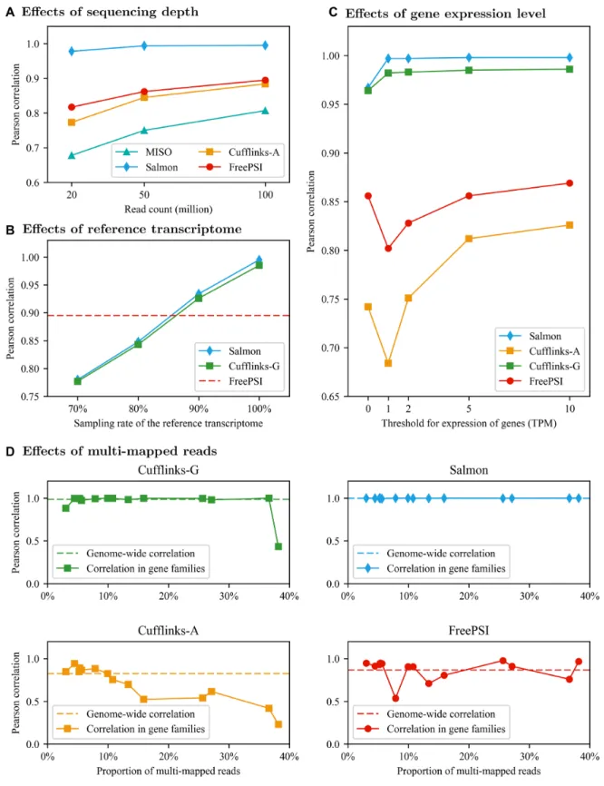
Sequencing depth is often considered as impact factor in RNA-seq analysis. In order to observe how sequencing
depth may affect the accuracy of the PSI quantification methods, we simulate two more RNA-seq datasets, with 20 million reads and 50 million reads each, respectively. The ac-curacy results of MISO, Salmon, Cufflinks-A, and FreePSI on all three simulated datasets are shown in Figure 4A. Clearly, the trend is the same for all the methods and the accuracy gets better when the sequencing depth increases. While Salmon maintained a high accuracy for all three se-quencing depths, FreePSI was able to achieve a decent cor-relation at 0.817 on the dataset with only 20 million reads. In other words, FreePSI can be used to provide a robust esti-mate of PSI values on RNA-seq data with a broad range of sequencing depths, especially when a high quality reference transcriptome is unavailable.
Impact of reference transcriptome
As shown in Table1, the performance of the transcriptome-guided methods dropped sharply in the real data exper-iment, although they were nearly perfect in the simu-lation experiment. On the contrary, the performance of transcriptome-free methods remained robust on both simu-lated and real datasets. A plausible explanation of the poor performance of the transcriptome-guided methods on the real dataset is the mismatch between the reference transcrip-tome and true transcriptranscrip-tome expressed in the data. In order to test how the PSI quantification methods are affected by the quality of the reference transcriptome, we conduct the following simulation experiment.
We use the simulated dataset with 100 million reads, but provide a randomly selected subset of isoforms from the RefSeqrefGeneannotation as the input reference transcrip-tome for Salmon and Cufflinks-G. In other words, the tran-scriptome used in the simulation (i.e. the RefSeqrefGene an-notation) is the true transcriptome, but we assume that only an incomplete reference transcriptome is known. We use the sampling rate of the reference transcriptome to represent the coverage of the true transcriptome. As shown in Fig-ure4B, the accuracy of Salmon and Cufflinks-G (measured by Pearson correlation) decreased almost linearly with the drop of the sampling rate. When the sampling rate de-creased to 80%, the performance of Salmon and Cufflinks-G was much worse than that of FreePSI.
In practice, reference transcriptomes are often incom-plete and many organisms do not have well-annotated tran-scriptomes. Hence, a plausible approach would be to as-semble the transcriptome first and then quantify PSI val-ues, as illustrated in Cufflinks-A. In order to test how the quality of quantification would impact PSI estimation, we conduct another experiment that applies one of the best iso-form abundance quantification methods, Salmon, to per-form quantification based on the transcriptome assem-bled by Cufflinks-A (denoted as Cufflinks-A-Salmon). As Supplementary Figure S5 demonstrates, Cufflinks-A and Cufflinks-A-Salmon performed very similarly on both sim-ulated and real data. This may suggest that the bottleneck of estimating PSI values without a reference transcriptome for methods based on transcript quantification is still the quality of transcriptome assembly. Given the difficulty of transcriptome assembly, transcriptome-free methods such
as FreePSI are expected to have important applications in the analysis of many real RNA-seq data.
Impact of gene expression level
The above genome-wide performance evaluation on simu-lated data focused on the performance of the methods on highly expressed genes (i.e. abundance≥10 TPM). To study how the expression level of a gene may influence the accu-racy of PSI estimation, we consider subsets of genes with abundance above various TPM thresholds (i.e. 0, 1, 2, 5 and 10) in the simulated data with 100M reads. The per-formance of the methods on these subsets of genes is shown in Figure4C. When the TPM threshold increases from 0 to 10, the accuracy measured by the Pearson correlation of all methods generally increases. Clearly, the expression level of a gene has significant impact on the performance of the two transcriptome-free methods (i.e. Cufflinks-A and FreePSI). More highly expressed genes are generally ex-pected to produce more reads and thus correctly assembled isoforms, which lead to more correctly estimated PSI val-ues. The accuracy of FreePSI is always better than that of Cufflinks-A for all the TPM thresholds. Interestingly, the performance of both methods decrease significantly when the TPM threshold increases from 0 to 1. This suggests that the methods are able to deal with unexpressed genes better than lowly expressed genes. This is true for Cufflinks-A be-cause when a gene is not expressed, no isoform will likely be assembled and thus all PSI values of the gene will be output as 0 (correctly) in our experiment. As for FreePSI, although an unexpressed gene may attract a few noisyk-mers, their effect will likely be diminished by the linear constraints in the EM algorithm and the post-processing step of FreePSI, leading to (correctly) estimated PSI values of 0 for the gene. The robust performance of transcriptome-guided methods (i.e., Cufflinks-G and Salmon) suggests that a correct ref-erence transcriptome is important to PSI estimation espe-cially for lowly expressed genes.
Impact of multi-mapped reads
Table 1 suggests that FreePSI provides a better esti-mate than Cufflinks-A and Salmon performs better than Cufflinks-G (and MISO) on simulated data. In other words, the alignment-free or pseudo-alignment-based methods generally perform better than the alignment-based meth-ods, with or without the reference transcriptome. The advantage of alignment-free and pseudo-alignment-based methods in PSI estimation can perhaps be explained by con-sidering the impact of multi-mapped reads. Cufflinks first uses uniquely mapped reads to estimate the relative abun-dance of isoforms and then employs a ‘rescue method’ to refine the estimates using multi-mapped reads. On the other hand, the alignment-free methods and pseudo-alignment-based methods do not distinguish multi-mapped reads from uniquely mapped reads, and use all reads simultaneously to perform quantification. We conduct a simple simulation ex-periment below to study the impact of these different treat-ments of multi-mapped reads on PSI estimation.
We consider the simulated dataset with 100 million reads again. Among all mapped reads, 2.48% are mapped to
mul-Figure 4. (A) Impact of sequencing depth. The figure shows Pearson correlation between estimated PSI values and the ground truth on the spliced exons (i.e. exon-centric evaluation) under various sequencing depths. (B) Impact of reference transcriptome. The X-axis represents the sampling rate used for creating the reference transcriptome for Salmon and Cufflinks-G. The Y-axis represents Pearson correlation between estimated PSI values and the ground truth on the spliced exons (i.e. exon-centric evaluation). The dashed line denotes the performance of FreePSI in the exon-centric evaluation as a reference. (C) Impact of gene expression level. The figure shows the Pearson correlation between estimated PSI values and the ground truth on expressed genes under different TPM thresholds. (D) Impact of multi-mapped reads. The four plots show the performance of four PSI estimation methods on 14 gene families with high proportions of multi-mapped reads. Each point represents Pearson correlation on all exons of the genes in the corresponding family. The X-axis represents the proportion of multi-mapped reads in each gene family. The dashed line denotes the Pearson correlation coefficient obtained by the method in genome-wide evaluation as a reference. The full details of all results discussed in this figure can be found in Supplementary Tables S1, S2, S3 and S4 of Supplementary Section S5.5.
tiple positions. Since multi-mapped RNA-seq reads are gen-erally from genes with similar sequences, we retrieve gene families from the HGNC database and consider large gene families that have large numbers of isoforms. These gene families are expected to result in large portions of multi-mapped reads in the simulated dataset with 100 million reads. Altogether, 93 gene families are selected, each of which contains>20 genes and at least twice as many iso-forms. Out of these gene families, 14 contain multi-mapped reads that are more than 2.48% of their total numbers of mapped reads. Figure 4D shows the accuracy of the PSI estimation methods on the 14 gene families with different proportions of multi-mapped reads.
While Salmon’s performance was robust across all gene families and remained nearly optimal, Cufflinks-G per-formed well on most gene families but failed to obtain an acceptable estimate of PSI values on the gene family with the highest proportion of multi-mapped reads. The per-formance of FreePSI fluctuated slightly on the gene fam-ilies around its genome-wide performance. However, the performance of Cufflinks-A clearly decreased with the in-creased proportion of multi-mapped reads. This simple ex-periment illustrates that the performance of alignment-free and pseudo-alignment-based methods are generally not affected by the existence of multi-mapped reads, but the performance of alignment-based methods may suffer from a proportion of multi-mapped reads. In particular, al-though the “rescue method” was enabled, without the guid-ance of the reference transcriptome, the performguid-ance of Cufflinks-A still suffered significantly from multi-mapped reads. Therefore, the advantage of FreePSI over Cufflinks-A is magnified on genes or gene families that involve large proportions of multi-mapped reads.
CONCLUSION
In this paper, we presented an alignment-free approach, FreePSI, for estimating exon-inclusion ratios (or PSI val-ues) without requiring the guidance of a reference transcrip-tome. FreePSI takes as its input a reference genome with exon boundary annotation and a set of RNA-seq reads, and produces the PSI values of all annotated exons. An abun-dance flow graph was introduced to represent all possible isoforms and their abundance levels. A novel probabilistic generative model was designed to allow for an alignment-free estimation of the parameters in the abundance flow graph. An efficient EM method based on a divide-and-conquer strategy was proposed to decompose a genome-wide MLE of the model into independent optimization sub-problems for each gene. An ultrafast optimization algo-rithm, conjugate gradient projection descent, was imple-mented for solving these subproblems in parallel. Finally, a post-processing procedure was adopted to smooth out the estimated PSI values in each gene.
FreePSI is the first quantification method achieving transcriptome-free and alignment-free simultaneously in RNA-seq data analysis. As a result, it not only performs well when high quality reference transcriptomes are not present, but also runs efficiently and is able to deal with data involving a large proportion of multi-mapped reads. We ex-pect that FreePSI will have important applications in the
alternative splicing analysis for organisms that do not have well studied transcriptomes.
AVAILABILITY
The FreePSI algorithm is freely available under the GNU General Public License (GPLv3). A version of the source code has been deposited at https://github.com/JY-Zhou/ FreePSI. The scripts for generating the simulated RNA-seq datasets analyzed in the paper can be found on the same GitHub page. The actual datasets and detailed experimen-tal results are available from the corresponding author upon request.
SUPPLEMENTARY DATA
Supplementary Data are available at NAR Online.
ACKNOWLEDGEMENTS
J.Z. and T.J. designed the model, algorithm and experi-ments. J.Z. implemented the program and conducted the experiments. D.W., S.M. and J.Z. (Jianyang) provided some useful advice. J.Z. and T.J. wrote the paper and all authors have reviewed the paper. We would like to thank Dr Rui Jiang (Tsinghua University) for the support of computa-tional resources, and the anonymous referees for many con-structive suggestions.
FUNDING
US National Science Foundation (in part) [DBI-1262107, IIS-1646333 to T.J.]; National Natural Science Foundation of China [61472205 to J.Z.]; Youth 1000-Talent Program of China (to J.Z.); Ningbo Science and Technology Dis-covery Grant [2014B82014 to T.J.]. Funding for open ac-cess charge: US National Science Foundation Grant [IIS-1646333].
Conflict of interest statement.None declared.
REFERENCES
1. Barash,Y., Calarco,J.A., Gao,W., Pan,Q., Wang,X., Shai,O., Blencowe,B.J. and Frey,B.J. (2010) Deciphering the splicing code.
Nature,465, 53–59.
2. Kakaradov,B., Xiong,H.Y., Lee,L.J., Jojic,N. and Frey,B.J. (2012) Challenges in estimating percent inclusion of alternatively spliced junctions from RNA-seq data.BMC Bioinformatics,13, S11. 3. Saltzman,A.L., Pan,Q. and Blencowe,B.J. (2011) Regulation of
alternative splicing by the core spliceosomal machinery.Genes Dev.,
25, 373–384.
4. Ohta,S., Nishida,E., Yamanaka,S. and Yamamoto,T. (2013) Global splicing pattern reversion during somatic cell reprogramming.Cell Rep.,5, 357–366.
5. Venables,J.P., Klinck,R., Koh,C., Gervais-Bird,J., Bramard,A., Inkel,L., Durand,M., Couture,S., Froehlich,U., Lapointe,E.et al.
(2009) Cancer-associated regulation of alternative splicing.Nat. Struct. Mol. Biol.,16, 670–676.
6. Barbosa-Morais,N.L., Irimia,M., Pan,Q., Xiong,H.Y.,
Gueroussov,S., Lee,L.J., Slobodeniuc,V., Kutter,C., Watt,S., C¸ olak,R.
et al.(2012) The evolutionary landscape of alternative splicing in vertebrate species.Science,338, 1587–1593.
7. Wang,Z., Gerstein,M. and Snyder,M. (2009) RNA-Seq: a revolutionary tool for transcriptomics.Nat. Rev. Genet.,10, 57–63.
8. Garber,M., Grabherr,M.G., Guttman,M. and Trapnell,C. (2011) Computational methods for transcriptome annotation and quantification using RNA-seq.Nat. Methods,8, 469–477. 9. Conesa,A., Madrigal,P., Tarazona,S., Gomez-Cabrero,D.,
Cervera,A., McPherson,A., Szcze´sniak,M.W., Gaffney,D.J., Elo,L.L., Zhang,X.et al.(2016) A survey of best practices for RNA-seq data analysis.Genome Biol.,17, 13.
10. Alamancos,G.P., Pag`es,A., Trincado,J.L., Bellora,N. and Eyras,E. (2015) Leveraging transcript quantification for fast computation of alternative splicing profiles.RNA,21, 1521–1531.
11. Trapnell,C., Williams,B.A., Pertea,G., Mortazavi,A., Kwan,G., Van Baren,M.J., Salzberg,S.L., Wold,B.J. and Pachter,L. (2010) Transcript assembly and quantification by RNA-Seq reveals unannotated transcripts and isoform switching during cell differentiation.Nat. Biotechnol.,28, 511–515.
12. Li,B. and Dewey,C.N. (2011) RSEM: accurate transcript quantification from RNA-Seq data with or without a reference genome.BMC Bioinformatics,12, 323.
13. Li,W. and Jiang,T. (2012) Transcriptome assembly and isoform expression level estimation from biased RNA-Seq reads.
Bioinformatics,28, 2914–2921.
14. Roberts,A. and Pachter,L. (2013) Streaming fragment assignment for real-time analysis of sequencing experiments.Nat. Methods,10, 71–73.
15. Li,W., Feng,J. and Jiang,T. (2011) IsoLasso: a LASSO regression approach to RNA-Seq based transcriptome assembly.J. Computat. Biol.,18, 1693–1707.
16. Pertea,M., Pertea,G.M., Antonescu,C.M., Chang,T.-C., Mendell,J.T. and Salzberg,S.L. (2015) StringTie enables improved reconstruction of a transcriptome from RNA-seq reads.Nat. Biotechnol.,33, 290–295.
17. Liu,J., Yu,T., Jiang,T. and Li,G. (2016) TransComb: genome-guided transcriptome assembly via combing junctions in splicing graphs.
Genome Biol.,17, 213.
18. Langmead,B., Trapnell,C., Pop,M. and Salzberg,S.L. (2009) Ultrafast and memory-efficient alignment of short DNA sequences to the human genome.Genome Biol.,10, R25.
19. Trapnell,C., Pachter,L. and Salzberg,S.L. (2009) TopHat: discovering splice junctions with RNA-Seq.Bioinformatics,25, 1105–1111. 20. Kim,D., Pertea,G., Trapnell,C., Pimentel,H., Kelley,R. and
Salzberg,S.L. (2013) TopHat2: accurate alignment of transcriptomes
in the presence of insertions, deletions and gene fusions.Genome Biol.,14, R36.
21. Kim,D., Langmead,B. and Salzberg,S.L. (2015) HISAT: a fast spliced aligner with low memory requirements.Nat. Methods,12, 357–360. 22. Patro,R., Mount,S.M. and Kingsford,C. (2014) Sailfish enables
alignment-free isoform quantification from RNA-seq reads using lightweight algorithms.Nat. Biotechnol.,32, 462–464.
23. Marc¸ais,G. and Kingsford,C. (2011) A fast, lock-free approach for efficient parallel counting of occurrences of k-mers.Bioinformatics,
27, 764–770.
24. Bray,N.L., Pimentel,H., Melsted,P. and Pachter,L. (2016)
Near-optimal probabilistic RNA-seq quantification.Nat. Biotechnol.,
34, 525–527.
25. Patro,R., Duggal,G., Love,M.I., Irizarry,R.A. and Kingsford,C. (2017) Salmon provides fast and bias-aware quantification of transcript expression.Nat. Methods,14, 417–419.
26. Katz,Y., Wang,E.T., Airoldi,E.M. and Burge,C.B. (2010) Analysis and design of RNA sequencing experiments for identifying isoform regulation.Nat. Methods,7, 1009–1015.
27. Shen,S., Park,J.W., Huang,J., Dittmar,K.A., Lu,Z.-X., Zhou,Q., Carstens,R.P. and Xing,Y. (2012) MATS: a Bayesian framework for flexible detection of differential alternative splicing from RNA-Seq data.Nucleic Acids Res.,40, e61.
28. Shen,S., Park,J.W., Lu,Z.-X., Lin,L., Henry,M.D., Wu,Y.N., Zhou,Q. and Xing,Y. (2014) rMATS: robust and flexible detection of differential alternative splicing from replicate RNA-Seq data.Proc. Natl. Acad. Sci. U.S.A.,111, E5593–E5601.
29. Heber,S., Alekseyev,M., Sze,S.-H., Tang,H. and Pevzner,P.A. (2002) Splicing graphs and EST assembly problem.Bioinformatics,
18(Suppl. 1), S181–S188.
30. Goldfarb,D. (1969) Extension of Davidon’s variable metric method to maximization under linear inequality and equality constraints.SIAM J. Appl. Math.,17, 739–764.
31. Griebel,T., Zacher,B., Ribeca,P., Raineri,E., Lacroix,V., Guig ´o,R. and Sammeth,M. (2012) Modelling and simulating generic RNA-Seq experiments with the flux simulator.Nucleic Acids Res.,40,
10073–10083.
32. NA,J. and JN,F. (2011) Sickle: A sliding-window, adaptive, quality-based trimming tool for FastQ files.