EEG Source Localization: A Machine Learning Approach

(1)

UNIVERSITY OF TARTU

Institute of Computer Science

Computer Science Curriculum

Gagandeep Singh

EEG Source Localization:

A Machine Learning Approach

Master’s Thesis (30 ECTS)

Supervisor: Ilya Kuzovkin, MSc

(2)

EEG Source Localization: A Machine Learning Approach

Abstract

There are different techniques for recording human brain activity. One of them EEG can capture brain activity in the time frame at which the activity occurs, but has a poor spatial resolution. Another technology fMRI, captures brain activity with high spatial resolution compared to EEG, but with poor temporal resolution. Simultaneously recording brain activity using these two techniques helps us capture a richer, spatio-temporally more precise description of human brain activity. Inferring the source location within the brain from an EEG signal is defined as EEG source localization problem. In this thesis, a new method that is based on machine learning for solving EEG source localization problem is proposed and its performance is evaluated on a simultaneously recorded EEG and fMRI data set. This method’s performance is also compared to a commonly used method.

Keywords:

Source localization, Brain, EEG, fMRI, Machine Learning, Deep Learning

(3)

EEG allika lokaliseerimine: masinaõppe lähenemisviis

Lühikokkuvõte:

Inimaju aktiivsuse salvestamise jaoks on olemas mitmeid meetodeid. Üks nendest on EEG, mis suudab ajusignaali mõõta peaaegu samal hetkel, kui see signaal ajus te-kib.Samas selle ruumiline täpsus on väga madal. Konkureeriv tehnoloogia on fMRI, mille ruumiline täpsus on hea, kuid ajaline täpsus madal. Mõõtes ajusignaale kasutades mõlemat tehnoloogiat korraga saab kätte signaali, mis on rikas ja täpne aju aktiivsuse kirjeldus nii ruumis kui ka ajas. Signaali allika järeldamist EEG andmetest nimetatakse allika lokaliseerimise probleemiks. Antud uuringus me demonstreerime uut lokaliseeri-mise meetodit, mis kasutab masinõpet. Uue meetodi suutlikkuse hindalokaliseeri-miseks kasutame andmestikku, kus EEG ja fMRI signaalid olid salvestatud samaaegselt. Samuti võrdleme antud töös väljatöötatud meetodit teiste allika lokaliseerimise meetoditega.

Võtmesõnad:

Allika lokaliseerimine, Aju, EEG, fMRI, Masinõpe, Sügav õpe.

CERCS:P170 Arvutiteadus, arvutusmeetodid, süsteemid, juhtimine (automaatjuhtimis-teooria)

(4)

Acknowledgements

First and the foremost, I would like to express my sincere gratitude towards the Institute of Computer Science for providing me with the resources and the opportunity to work on this thesis.

I would like to thank my thesis supervisor Ilya Kuzovkin for his guidance, patience and the motivation he provided all along, to meet the goals of the thesis. I am also thankful to all of the staff members of the Institute of Computer Science and HPC center for providing support and help whenever I needed.

My sincere thanks go to all of my friends in Estonia, back home and abroad, for their constant encouragement and love.

Finally, I would like to thank my parents, Smt. Amarjeet Kaur and Shri. Krishanpal Singh, and the rest of my family for their love and support not just during my thesis work, but also throughout my life.

(5)

Chapter 1 Introduction

1.1 Context

Human brain continuously generates electromagnetic signals. The localization of the active brain areas which are responsible for those signals is termed as brain source localization. This process of source estimation with the help of Electroencephalography (EEG) is known as EEG source localization problem. Solving the EEG source localization problem requires solving the forward and the inverse problem. Solving the forward problem requires estimating the potentials at the electrodes on the scalp, given some source distribution inside the head. Forward problem is solved repeatedly for different distributions of the source(s). EEG inverse problem is solved using the forward solution, to estimate the distribution of source(s) from an EEG recording .

1.2 Why solving EEG source localization is important?

Once solved, EEG source localization is helpful to understand physiological, pathological, mental, functional abnormalities and cognitive behavior of the brain. This understanding leads to the specification for diagnoses of various brain disorders such as epilepsy and tumor.

1.3 Challenges in solving EEG source localization

The human brain is the most complicated organ in the human body. Although realistic head models have been invented, solving the forward problem using them requires a large number of calculations. Iterative methods need to be used for approximating the solution of the forward problem, which are computationally expensive [20]. On the other hand, the inverse problem is an ill-posed problem, because number of possible source

(8)

locations is much higher than the number of parameters. For example, let’s say we have

psources in the brain and we useN electrodes to estimate the location of thesepsources. Sincep >> N, so we will have less equations to solve for more unknowns. So the solution to the inverse problem will usually not be unique.

1.4 General approaches

For solving the forward problem, simple model or realistic head models are used. An example of a simple head model is spherical three-shell model. Realistic head models use numerical methods like the boundary element method (BEM), the finite element method (FEM) and the finite difference method (FDM). Sources are modeled as a dipole. There are two classes of methods used for solving inverse problem: (a) parametric and (b) non-parametric [20].

1.5 Proposed method

In this thesis, a new method to solve EEG source localization problem is proposed. Using a data set where EEG and functional magnetic resonance imaging (fMRI) were simultaneously recorded, the problem is reformulated as a supervised machine learning problem. Availability of fMRI data allows to eliminate the need for solving the forward problem by providing an estimate of the true sources. True source for an EEG can be estimated from an fMRI volume by dividing it intoBrodmann areas(BA). The hypothesis tested in this thesis is : given a data set, where each example is of the form (Xi, Yi) where eachXi= EEG for single stimulus and eachYi is corresponding brain area, extracted from fMRI image(s), can a machine learning model, learn to identify the brain area where the EEG signal originated from?

1.6 Thesis structure

This thesis is constructed as follows: in Chapter 2, we review the theoretical concepts, which are used in this thesis. In Chapter 3, we discuss the EEG source localization problem in detail and reviews the literature for related work, where machine learning approaches are applied to solve the forward and inverse problems. In Chapter 4 we describe the data set used and the proposed method in detail. Chapter 5 presents the results of different machine learning methods, used in this thesis to solve EEG source localization problem and compares results to a commonly used method.

(9)

Chapter 2 Theoretical background

In this chapter, the mechanisms by which EEG and fMRI sginals are generated are described and the theory behind the machine learning methods used in this thesis is discussed.

2.1 Electroencephalography(EEG)

2.2 EEG physics

The human brain consists of 106 _{neurons. Each neuron has a nucleus, dendrites, and}

axons. Dendrites receive inputs from other neurons, wheres axons form synapses with other neurons. Through axon, the neuron passes its electrical activity to other neurons. When a neuron fires, the action potential of 70–110 mV is generated, which is sufficiently large for measurement, but it lasts for a really short time (0.3 ms). It’s unlikely that neighboring neurons will fire synchronously. The postsynaptic potentials generate an extra-cellular potential field, which has a longer time course (10–20 ms). This allows for summed activity of neighboring neurons. However, their amplitude is smaller (0.1–10 mV). The electrodes used for recording EEG are large and sparse and can only detect combined activities of a large number of neurons which are synchronously active. EEG records the activity from postsynaptic potentials [20]. Figure 2.2.1 shows structure of a neuron.

For EEG to pick up the signal generated by the neurons, their spatial arrangement must be such that they amplify each other’s extra-cellular potential field, in addition to their synchronous activity. The neighboring pyramidal cells are organized so that the axes of their dendrite tree are normal to the cortical surface and parallel to each other. Hence, pyramidal cells are believed to be the generators of the EEG. These cells are modeled as electrical dipoles [20].

(10)

Figure 2.2.1. Structure of a neuron [1].

2.2.1 EEG signal

EEG is the method to record the electrical activity of the brain. EEG provides non-invasive access to brain activities. An example of an EEG recording system and a signal is shown in Figure 2.2.2:

Figure 2.2.2. An illustration of EEG electrodes and signal [2].

EEG signal is recorded by placing a set of small discs, called electrodes, on the scalp. These electrodes pick up the electrical activity from the pyramidal neurons. The arrange-ment of these electrodes on the scalp while recording is important. Usual placearrange-ment systems are 10-20 system and 10-5 system, where electrodes are arranged at 10% and 20% points along lines of longitude and latitude on the scalp.

(11)

Based on the frequency of the recorded signal from EEG, brain waves are divided into 5 bands: 0.5–4 Hz (delta,δ) 4–8 Hz (theta,θ), 8–13 Hz (alpha,α), 13–30 Hz (beta,β) and >30 Hz (gamma,γ). EEG signal might be contaminated due to signals from non-cerebral signals. The common artifacts are due to blinking, electrode movement, swallowing and head movement [2].

2.2.2 EEG signal processing

There are many methods described in the literature for processing EEG signals. However, Wavelet transform will be reviewed here, as it is used in this thesis.

Wavelet analysis finds an alternative representation of a signal into a set of basis functions using wavelets. Wavelets are generated in terms of translations and dilations of a fixed function calledmother wavelet. Wavelets are well localized in time and frequency and are useful for non-stationary signal analysis.

2.3 Functional Magnetic Resonance Imaging(fMRI)

fMRI is used for taking high-resolution brain images compared to EEG and measures neuronal activity indirectly. The idea behind the fMRI signal is that when a particular region of the brain is active, the blood flow to that region increases. So the fMRI signal measures the neuronal activity by measuring the blood flow through different brain areas and is thus called BOLD:Blood Oxygenation Level Dependentsignal. In this section, the theory behind 3D fMRI image generation and different fMRI coordinate systems are discussed. The material is based on the coursera course:"Principles of fMRI 1".

2.3.1 Magnetic resonance physics

The magnetic field produced by a moving chargeqis given by[4]:

~

B = (µo/4π)∗((q~v×~r)/r3) (2.3.1)

where,B~ = Magnetic field produced by the moving charge,q= The moving charge,~r= A vector from charge q to the point where we wish to measure the magnetic field,~v = Velocity of the moving charge.

Around 60 percent of the human body is made up of water, which provides major the source of protons, the positively charged particles in our body. Protons have smaller charge, but they do move really fast, thus creating a small magnetic field. Under normal conditions these small magnets (protons), are randomly aligned, giving net zero magnetic field, as is shown in Figure 2.3.1.

(12)

Figure 2.3.1. Protons aligned randomly with no magnetic field

When a strong enough magnetic field is applied to the protons, some of them will align with the magnetic field and some will align in opposite direction of the applied magnetic field. However, if the magnetic field is strong enough, more protons will be aligned in the direction of magnetic field, giving result to a net magnetic field as is shown in Figure 2.3.2.

Figure 2.3.2. protons aligned with the magnetic field

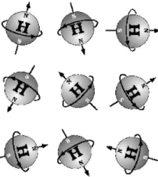
If we apply the magnetic field on z-direction, then the protons align themselves into some angle with z-axis, giving rise to a magnetization which has longitudinal and transverse components. Longitudinal is in z-direction and transverse is in the x-y plane, which is perpendicular to the applied magnetic field. The protons while aligned with the external magnetic field also precess or wobble with an angular frequency called Larmour Frequency but at different phase with respect to each other as is shown in Figure 2.3.3.

(13)

Figure 2.3.3. Protons precessing in different phase [5]

When we apply a radio frequency (RF) pulse, it aligns the protons in phase and then tips them over, giving net rise to the magnetic field in the transverse direction as is shown in Figure 2.3.4 and 2.3.5.

Figure 2.3.4. Protons precessing in the same phase and after RF pulse [5] .

Figure 2.3.5. Protons precessing in same phase tipped after RF pulse [5] .

Once we remove this RF pulse, the system tries to reach to equilibrium and the transverse magnetic field starts to decrease and longitudinal field start to grow back to its original value. The process of longitudinal field growing back to its original value is calledLongitudinal Relaxation, which is exponential growth described by the time constant T1 and is shown is Figure 2.3.6.

(14)

Figure 2.3.6. The relaxation time of different tissues [5] .

The loss of transverse magnetic field is calledTransverse Relaxationand is described by time constant T2 and is shown in Figure 2.3.7.

Figure 2.3.7. Time Constant T2 [5] .

There is another time constant called T2*, which is the combined effect of T2 and local inhomogeneities in the magnetic field.

The generated signal is given by below equation:

S(t) =Mo(1−e−T R/T1)∗e−T E/T2 (2.3.2)

whereT R= Repetition Time and is defined as the time after which we repeatedly excite the protons. T E = Echo Time and is the time after excitation, after which we start recording the signal.

By altering TR and TE in above equation, we can focus on different characteristics of the tissue. For example, if we choose a long TR and a short TE, we are going to get

(15)

a proton density image ad if we choose a long TR and long TE, we get a T2 weighted image. Whereas if we choose a short TR and short TE we will acquire a T1-weighted image. Figure 2.3.8 summarize this.

Figure 2.3.8. Different Image Contrasts.[5]

When we record a fMRI image, the brain is assumed as a 3D cube and then the image is acquired by taking 2D slices of this cube.. Each slice is further divided into equally sized volume elements or voxels. Figure 2.3.9 shows how we divide the brain into a 3D cube and slices [6].

Figure 2.3.9. fMRI 3D volume slices [6] .

Let’s say we wish to measure the density at position x,y in a slice as shown below in Figure 2.3.10:

(16)

Figure 2.3.10. Voxel example.[6]

The signal we will acquire will be the combined signal from whole brain i.e. we can integrate over and can be expressed as:

S(t) =

Z Z

ρ(x, y)dxdy (2.3.3) The magnetic field is changed sequentially to account for the spatial in-homogeneities and signal is measured in the frequency domain, which is represented mathematically as:

S(kx, ky) =

Z Z

ρ(x, y)e−i2π(kxx+kyy)_dxdy _(2.3.4)

The acquired signal is called in K-space. By doing enough measurements for different

kxandky values the inverse problem can be solved andρ(x, y)can be calculated using

inverse Fourier Transform equation

ρ(x, y) =

Z Z

S(kx, ky)ei2π(kxx+kyy)dxxdyy (2.3.5)

Since making the measurement for continuous values ofkx andky is not practical,

they are measured discretely over a finite region and discrete Fourier Transform is used to calculateρ(x, y). The number of K-space measurements define the spatial resolution of the acquired image, but the measurements must also be enough to solve the inverse problem. The measurements made in K-space are complex valued as is clear from the above equation. In practice we work with magnitude images, which can be described by below equation:

|ρ(x, y)|=pρR(x, y)2+ (ρI(x, y)2 (2.3.6)

WhereρR(x, y)andρI(x, y)are real and imaginary parts of k-space measurement.

Figure 2.3.11 summarize how K-space measurementskx andky creates an image

(17)

Figure 2.3.11. K-space and Image-space.[6]

Figure 2.3.12 summarize how discrete points sampled in K-space leads to image resolution.

2.3.2 fMRI coordinate systems

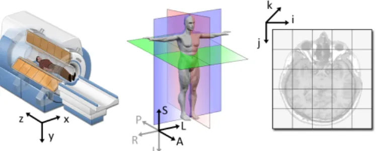
There are three coordinate systems used in fMRI images [7]:

World coordinate system: A Cartesian coordinate system in which we can define the position and orientation of any object in the world. There is only one World coordinate system and each point is represented by three symbols (x, y, z). It is also called the scanner coordinate system.

Anatomical coordinate system:This is the 3D coordinate system defined using the patient as the reference and it has 3 planes to describe any point:

• the axial plane is parallel to the ground and separates the head (superior) from the feet (inferior).

• the coronal plane is perpendicular to the ground and separates the front from (anterior) the back (posterior).

• the sagittal plane separates the left from the right.

The 3D basis are defined along the anatomical axes of anterior-posterior, inferior-superior, and left-right. Most commonly used basis are:

(18)

• LPS (Left, Posterior, Superior):the coordinates are measured from right to left, then from anterior to posterior and then from inferior to superior.

• RAS (Right, Anterior, Superior): the coordinates are measured from left to right, then from posterior to anterior and then from inferior to superior.

Figure 2.3.12. K-space and image space resolution [6] .

Image coordinate system:This coordinate system defines the coordinates of an acquired image with respect to the image. The top left corner is defined as the origin and the coordinates of each point are defined by symbols, (i, j, k).

Figure 2.3.13 shows the three coordinates systems and how they differ in their definition of origin and location and orientation of each point:

Figure 2.3.13. fMRI Coordinate Systems. First is the world,the middle is Anatomical and last is image coordinate system [7]

(19)

2.4 Machine learning methods

2.4.1 Random forest

Random Forest is a class of methods in machine learning which are used for classification and regression and use ensemble methods. Random Forest was developed byBreimen

[8] in 2001 and consist of a bunch of weak decision trees and combine their predictions using bagging to determine the class label of an unlabelled instance. RF are used because of their powerful prediction power and simplicity to understand. Figure 2.4.1 [9] shows an example of a random forest.

Figure 2.4.1. Random Forest example [9] .

Above RF is created to figure out if a kid can go out to play or not based on weekend,outlook and hwdone. For example, the kid can go to play if its weekend.

Breimanalso introduced the classification and Regression trees(CART) technique to introduce additional randomness in RF. In CART technique the next feature to split is decided using a criterion called Ginni Index, which is defined as [9]:

Gini(t) = 1−

N

X

i=1

P(Ci|t)2 (2.4.1)

where,t = condition,N = no of classes in the data set,Ci is the ith class label. Figure

2.4.2 [9] lists the RF algorithm, where N is the number of samples and S is the number of features.

(20)

Figure 2.4.2. RF Algorithm [9] .

2.4.2 Convolution Neural Networks (CNN)

CNN are different than traditional neural networks in the sense that they are engineered to work on images by design and to ensure some degree of shift, scale and distortion invariance. They use three ideas to achieve them: local receptive fields, shared weights, and spatial sub-sampling. By using these ideas CNN reduces the number of parameters to learn and leads to faster learning times. Each successive convolution layer in CNN learns higher level features.

There are four main layers in a typical convolution neural net [10]:

1. Convolution Layer: In a convolution layer, a small kernel or a filter forms a feature map by sliding this kernel over the image and computing the dot product. The most important feature of CNN is that the filters are automatically learned by CNN based on the training data. There are three parameters which define the feature map:depththe number of filters to use,stridepixels count by which we slide our filter over input image andzero paddingits useful sometimes to append 0’s at the border of the image so that we can apply our filter to the edges of the image.

2. Non-Linearity:Since convolution is a linear function and most real-world data is non-linear, we apply a non-linearity in CNN, after every convolution layer. There

(21)

are many non-linearities available in the literature. The most commonly used one’s are:Relu, Tanh, sigmoid etc[11].

3. Sub-Sampling/Pooling Layer:Sub-Sampling layer reduces the size of the output of convolution layer, keeping the most useful information. Since the output of convolution after applying non-linearity will be a matrix of numbers, sub-sampling reduces this matrix into a single number, thus keeping most useful information. Sub-sampling could of different types:Max, Sum, Average etc.. Figure 2.4.3 shows an example of sub-sampling.

Figure 2.4.3. Max-Pooling operation CNN [10] .

4. Fully Connected Layer: Fully connected layer is a layer which connects each neuron to every neuron in the previous layer. The common activation used for fully connected layer is softmax. Fully connected layer uses the high-level features derived from the previous layers as input and produces a class label as an output in binary classification.

The Figure 2.4.4. shows LeNet-5 architecture, which was once a state of the art CNN:

(22)

Figure 2.4.4. Le-Net 5 Architecture.[12]

2.4.3 Autoencoders

An autoencoder is a supervised learning algorithm that is trained to copy its input to the output. It has a hidden layerh, that is used to represent the input and usually, the hidden layer’s size is smaller than the input. The network has two parts: an encoder function

h = f(x)and a decoder function d = g(h), that produces a reconstruction from the encoded input. This architecture is presented in figure 2.4.5

Figure 2.4.5. A linear autoencoder [17] .

Let’s assume we have a neural network with inputx(i)_{, a single hidden layer with}

linear activation, and outputxˆ(i)then the hidden layer activations,z(i)and the output can be represented as:

z(i)=W1x(i)+b1 (2.4.2)

ˆ

x(i)=W2z(i)+b2 (2.4.3)

whereW1 is the weight vector from input to hidden layer andW2 is the weight vector

(23)

As we wish to have xˆ(i) _{to approximate} _x(i) _{, we can simply use sum of squared}

differences betweenxˆ(i)andx(i)as our objective function:

J(W1, b1, W2, b2) =

M

X

i=1

(ˆx(i)−x(i))2 (2.4.4) which we can minimize using gradient descent or any other minimization algorithm [13]. For a non-linear data set, we can use non-linear activations in the hidden layer. Au-toencoders have many interesting applications, which include one-class classification, dimensionality reduction, visualization, data denoising, weight initialization for deep networks etc.

2.4.4 ADASYN & SMOTE

ADASYN&SMOTEare techniques for balancing, imbalanced data sets. ADASYN stand for adaptive synthetic and is sampling technique. SMOTE stands for synthetic minority over-sampling technique. A data set is imbalanced if the classes are not approximately equally represented. For example, data points for different kinds of cancers are normally very rare compared to normal non-cancerous cases; therefore, the ratio of the minority class to the majority class can be significant. Both ADASYN and SMOTE generate synthetic data points using similar algorithm. Considering a samplex, a new sample

xnew is generated considering its k neareast-neighbors. Then, one of these

nearest-neighborsxziis selected and a new data point,xnewis generated using below formula:

xnew=xi+λ×(xzi−xi) (2.4.5)

whereλis a random number in the range [0, 1].

The major difference between SMOTE and ADASYN is that how many data points are generated for each minority class data point. There are many variants of SMOTE, but the regular SMOTE method will generate new data points for randomly picked up minority class data points. ADASYN on the other hand will generate new data points, for the minority class samples which has more majority class samples as neighbours. [14] [15].

2.4.5 Performance metrics

After training a machine learning model on a data set, the next step is to evaluate how effective is the model using some performance metric. Different performance metrics are used to evaluate different Machine Learning Algorithms. For classification F1-score is commonly used performance metric. F1-Score is defined as the harmonic mean of precision and recall of the classifier. Precision is defined as :

(24)

where FP = false positive, and are cases the model incorrectly labels as positive that are actually negative. TP = true positive and are cases the model correctly labels as positive that are actually positive. Recall is defined as:

recall =T P/(T P +F N) (2.4.7) where FN = false negative and are data points the model identifies as negative that actually are positive.

(25)

Chapter 3 Problem statement and related work

In this chapter first the forward and inverse problems are reviewed and then literature survey is done for the related work.

3.1 Problem of EEG source localization

EEG Source localization is defined as a problem, where given voltage recordings from a set of electrodes at the scalp, we solve for the location of the sources of these voltages in the brain. These voltages are the result of currents flowing through the brain due to neural activity [16]. To solve the source localization problem, first, we need to have knowledge about the number and location of sources of these observed voltages. This is called forward problem. In general model of current sources in the brain, sources in different regions contribute to electrode voltages by summing linearly, as shown in Figure 3.1.1 [17].

EEG source localization is an ill-posed problem. The estimated number of sources in the brain by a model is much greater than the number of electrodes used to observe them, so we have fewer parameters to estimate the location and position of sources. This leads to a non-unique solution. To make a solution unique, we make assumptions and put constraints on the solution. For example, we put a constraint that the solution is of the minimum norm in the sLORETA method or by imposing covariance constraints on the solution in beamforming techniques [17]. Since we make assumptions about the sources in different methods, some solutions can never be found, no matter what experiment is performed or what EEG data is produced [18].

(26)

Figure 3.1.1. EEG sources linear combination [17] .

Mathematical formulation: Mathematically, EEG forward problem is defined as finding the potentialg(r, rdip, d), due to a single dipole, having dipole momentd=ded

and position vectorrdip, at an electrode on the scalp, having a position vectorr, as is

shown in figure 3.1.2. For more than one dipole the electrode potential would be [16]

m(r) =X

i

g(r, rdip_i, di) (3.1.1)

we are assuming a concentric three-shell head model. Since the dipoles are often constrained to have a normal orientation to the surface[19, 20], the potential will depend on the magnitude of the dipole moment and not on position of the dipole. So forN

electrodes,pdipoles atT discrete times, equation 3.1.1 [16] can be written as:

M =    m(r1,1) . . . m(r1, T) .. . . . . ... m(rN,1) . . . m(rN, T)   =    g(r1, rdip₁)e1 . . . g(r1, rdip_p)ep .. . . . . ... g(rN, rdip1)e1 . . . g(rN, rdipp)ep       d1,1 . . . d1, T .. . . . . ... dp,1 . . . dp, T    (3.1.2)

which can be written in general form as[16]:

M =GD (3.1.3)

whereM is the matrix for potentials at different electrodes on the scalp,Gis the gain matrix, also called the lead field.Dis the matrix of dipole moments at different times.

(27)

To account for uncertainties a noise matrix N is added to the system, so equation 3.1.3 [16] in general form can be written as:

M =GD+N (3.1.4)

It is clear from the equation 3.1.4, that to find the inverse solution, we need to find the estimateDˆ , of the matrixD, givenM andG.

Figure 3.1.2. The spherical model of the head[16].

As to get the inverse solution for EEG source localization, we need to solve for the forward problem, in the next subsections different approaches and methods to solve the forward and the inverse problem will be reviewed.

3.1.1 Forward problem

Hans et al [20] provides a complete overview and a mathematical treatment of the forward problem in EEG. Here, a brief overview is provided for completeness based onHans et al[20]. There are three models which must be known to solve the forward problem: (a) The source model (b) The head model and (c) The forward calculation model [21].

The source model

As is described in the section on EEG physics, the source of measured EEG are the pyramidal cells. These sources are modeled as a dipole. Since the activated area of the cerebral cortex may be larger, it can be modeled by a layer of dipoles.

The head model

(28)

and how this environment affects the potential measured at a distance from the source. Commonly used head models areuniform sphere model, concentric three-shell model, and complex models. The uniform sphere modelapproximates the head by assuming it to be a sphere of the uniform conducting material. The concentric three-shell model, represents the brain, skull and the scalp as three spherical concentric shells, with different conductivities.Complex modelstry to model the head as close to the real head as possible and are called the realistic head models.

The forward calculation method

The potential at an electrode on the scalp, using different head models is described by thePoisson’s equation[20]. Poisson’s equation is a continuous partial differential equation, so numerical methods are used to approximate the solution. Different methods used for solving Poisson’s equation in EEG include Boundary element method (BEM), Finite difference method (FDM) and the Finite element method (FEM). These methods use complex head models. BEM divides the brain into homogeneous and isotropic compartments using triangles and uses boundary conditions to solve the Poisson’s equation. The tissue types, which are used as the basis for the division are brain, skull and the skin. FEM divides the head using tetraeders and assumes non-uniform conductivity. More tetraeders are used where potential changes are rapid and less where potential changes are relatively stable. FDM coverts the Poisson’s equation into a set of algebraic equations by approximations obtained by Taylor expansions. Forward, backward, and central difference approximations could be used. FDM differ from the BEM and FEM method as FDM need to account for the source model whereas, BEM does not use the source model.

3.1.2 Inverse problem

An excellent review and mathematical treatment of inverse methods have been provided by Riberta et al [16]. Here a brief overview is provided for completeness based on

Riberta et al[16].

There are two classes of methods used for solving inverse problem: (a) parametric and (b) non-parametric. In parametric methods, a fixed number of dipoles is assumed a priori. Parametric methods capture all the information about the model in some parameters and once the model is built, data is not required anymore. In non-parametric methods, the model uses the current state of the data and the parameters for locating the sources. Non-parametric methods are also called distributed source Models.

Some commonly used non-parametric methods are minimum norm estimates and their generalizations, low resolution electrical tomography (LORETA), standardized low resolution brain electromagnetic tomography (sLORETA) and local autoregressive average (LAURA). Some parametric methods are beamforming techniques, brain elec-tric source analysis (BESA), subspace techniques such as multiple-signal classification

(29)

algorithm (MUSIC) and methods derived from it, artificial neural networks and genetic algorithms.

Non-parametric methods

Minimum norm estimate methodsare used in conjunction with distributed source models and search for the solution with minimum power using Tikhonov regularization. Com-pared to minimum norm estimate methods,LORETAallows to recover sources which are located deep in the head. Since LORETA is based on the maximum smoothness of the solution, it allows the source close to the surface and deeper ones, the same opportunity of being identified.sLORETA standardizes the current density estimate given by the minimum norm estimate by using its variance, to locate the sources. LAURAmethod includes Maxwell’s laws of the electromagnetic field, which states that source strength is inversely proportional to the cube of the distance for vector fields and to the square of the distance for the potential fields, into the minimum norm solution. The idea is to include biophysical laws into the minimum norm solution, which other minimum norm approaches does not include.

Parametric methods

Beamformersare also called spatial filters. In beamforming approaches, a set of weights are used to spatially filter the EEG data to estimate the source power for a specific location in the brain. BESA method minimizes a cost function which is weighted combination of four criteria: the Residual Variance (RV) is the signal which is unexplained by the current source model; a source activation criterion which is directly proportional to the source activity outside of their a priori time interval of activation; an energy criterion which avoids one source to compensate the other; a separation criterion in which as few sources as possible are simultaneously active. In MUSIC method, in the case of a dipole with the fixed orientation, a source is located by scanning its projections onto the signal subspace, which is calculated by the singular value decomposition(SVD) of the data.

Artificial neural networks (ANN)are robust to the noise in data, so they are used to solve the inverse problem by formulating it as a minimization problem. Genetic algorithms

use evolutionary techniques for solving the inverse problem as a minimization problem.

3.2 Related work

Commonly used methods for solving EEG source localization are computationally expensive and are iterative, which renders them impractical for clinical applications. Machine learning methods, once trained needs only one-step calculation to locate sources, for a new sample, thus they can be easily employed in clinical applications.[21]. This section describes various machine learning methods used in literature for solving EEG source localization problem.

(30)

3.2.1 Re-formulation of the problem for applying machine learning

In general machine learning methods have a defined set of steps which are taken to solve a particular problem. Most authors [21, 22, 23, 27, 28, 29, 30, 31], solve the forward problem using one of the classical methods and then use one of the machine learning methods to solve the inverse problem. However, authors in [25] and [26] have solved both the forward and inverse problem using machine learning methods. Minguiet al

[25] and Robertet al[26] solve the forward problem by mapping forward solution in a base spherical head model to a complex sphereoidal model (human head is close in shape to a spheroid), using artificial neural networks(ANN). The idea is to reduce the computational cost and reduce errors introduced by spherical head model. It is possible to use the spherical and spheroidal models to generate training data for ANN, as both models have analytical closed form solution.[25, 26]. Once the forward model is selected, [21, 22, 23, 27, 28, 29, 30, 31] use this model to generate training data for different models used for solving inverse problem in respective studies.

3.2.2 Approaches

Forward problem

Studies in [25, 26] have reported solving the forward problem using artificial neural networks. Complexities and differences of human head demands use of realistic head models. In these studies, authors learn a mapping function from analytically calculated electrode potentials from simple spherical head model to complex spheroidal model. Spheroidal model approximates the human head well. With suitable data and careful training, ANN’s can generalize to map the potentials of the spherical model to that of a set of spheroidal model. Thus ANN can be used to map from spherical model to any arbitrary spheroid that is not present in the training set, so renders it possible to use the same model for different subjects.

The relationship between the current source(s), head model and the measured poten-tials at the electrodes is given by the Poisson’s equation:

∆.(σ(r)∆φ(r)) = s(r) (3.2.1) forrΩ.

where∆is the gradient operator. φ(r)is the potential function of spatial vector r,

σ(r)is the conductivity tensor,s(r)is the current source density function andΩspecifies the ‘boundary conditions’.

In general, the shape of the head is not much different in the regions where we place the electrodes on the head for measuring EEG. As a result, computed potentials on the spherical and spheroidal head are highly correlated. Based on this condition, the authors in [25, 26] suggest a relationship between the potentials calculated for the spherical and

(31)

spheroidal models as:

φ2(Ω + ∆Ω, σ+ ∆σ, s) =f(∆Ω,∆σ, φ1(Ω, σ, s)) (3.2.2)

whereφ1 andφ2 are the potentials for the spherical and the spheroidal model. Then they

use ANN for approximating this function as described in below paragraphs, as ANN’s are universal function approximator’s [24] and there does not exist an analytic solution in general for equation 3.2.2.

The spherical head model the authors in [25] and [26] used is a sphere whose equation is :

x2+y2+z2 = 1 (3.2.3) A spheroid is an ellipsoid in which two of the three axes are equal. The equation representing a spheroid can be written as used in these studies is:

(x2+y2)/(1−η2) +z2 =a2 (3.2.4) where x, y, z are the Cartesian coordinates, η eccentricity of the ellipsoid, which is defined asη=p1−(a2_/b2_{). where}_b_{is long axis in the z-direction. For simplicity, the}

authors in [25] and [26] have usedb = 1and by experimentation with different head shapes, the authors have foundηto be between 0.4 to 0.6, for approximating ’true’ head model from spheroidal model [26]. If both models are aligned in the same coordinate system, then the corresponding electrode, (e, eη) and dipole positions (d, dη)can be

defined by a straight line connecting them to the originc, as shown in Figure 3.2.1.

Figure 3.2.1. Relationships between electrode locations (e, eη) and between dipole

locations(d, dη)for the spherical model and the spheroidal model [25]

(32)

12000 dipoles were randomly generated within the brain region of the spherical head model (|d|<0.84). Each dipole position,dwas mapped to corresponding dipole position

dη, on the spheroidal model. Also, 20 electrode positionsewere mapped toeη. Using

the analytical solutions for the spherical and the spheroidal model, training data for the ANN was generated, where the input corresponds to the electrode potentials,φ1(r)from

the spherical model and the output was the difference between the electrode potential from the spheroidal model,φ2(r)andφ1(r). The outputφ2(r)can be easily calculated

from the output of the ANN andφ1(r). The training set consisted of 12000 examples

and test set had 5000 examples.

In order for the ANN to adapt to different eccentricities of the spheroidal head model,ηwas included as an additional element in the input training vector. The ANN architecture used in both studies had an input layer with size 21 (input electrodes, and

η), a hidden layer with 30 neurons with sigmoid activation and an output layer with 20 neurons with linear activation. The architecture is shown in the figure 3.2.2.

Figure 3.2.2. ANN architecture used in forward study.

The metric used to evaluate the ANN model called therelative errorwas defined as:

E = Σ M i=1(φ2(i)−φˆ2(i))2 ΣM i=1φ2(i)2 ∗100% (3.2.5)

whereφ2 andφˆ2 are the directly computed and ANN predicted potentials respectively.

Five different algorithm were used for training the ANN and their results were evaluated using the above metric and are shown the Figure 3.2.3.Powell-Bealemethod was the fastest method to minimize the error. All the methods perform well.

(33)

Figure 3.2.3. Results for forward method using ANN.

Inverse Problem

In studies where the forward problem is not solved using ANN, the three concentric shells head model is most commonly used. [21, 22, 23, 27, 28, 29, 32]. However minor differences exist in the forward model, for example, [23] also experiment with the realistic head model, derived from 3D MR images and [29] uses four concentric shells. [30] and [31] do not mention directly, but it can be inferred from the text, that they also use spherical three concentric shells head model. Once the forward model have been selected: either ANN or spherical three-shell model, using ANN for inverse problem is straightforward. Generate training examples from either analytical solution from the spherical model or from ANN and train the ANN.

Three different machine learning methods have been used in literature for solving inverse problem: Artificial neural networks (ANN), Support vector machines (SVM) and genetic algorithms.

Artificial neural networks

Studies in [21, 22, 23] used a single dipole source, whereas [28] and [29] use two dipole sources to generate electrode potentials at the scalp. [26], uses three different source models: single dipole, a disc source model, and a line source model. Different studies used different approaches for data generation, models, evaluation metrics, and to present results. Only one study [21] which does a comprehensive work on the inverse problem is described here.

In the article by Udanthaet al[21], the authors used a three-shell spherical model to model the head. They used a single dipole source model . A 39 electrode grid was used for recording EEG. The six dipole parameters were taken as the output of the data generation step. So each training example had scalp voltage as input and 6 dipole parameters as output. The training set size was 1000 ~3000 whereas for testing 1000 examples were used.

(34)

trained on this data set. Network A and B had 39 neurons in input layer, 60 and 20 in respective hidden layers and 6 in output layer. The only difference between networks, A and B was that in network B, a Gaussian noise was added to test for the generalization of the ANN in case of low signal to noise ratio (SNR). Network C had 30 and 15 neurons in the two respective hidden layers and used the training data set that had been pre-scaled to a scaling level of 0.06. The output of each network, corresponds to the 6 parameters of the dipole, three for position and three for dipole moment.

Initial learning rate was set to 0.001 and then was decreased by multiplying it with 98% of its value if the training error was increasing. Dipole position error and dipole moment error, as defined below, were used, to asses the networks:

Dipole position Error:

DP E =

p

((x−χ)2_{+ (}_y₋_ψ₎2_{+ (}_z₋_ξ₎2₎

R ∗100% (3.2.6)

where, (x,y,z) : Actual dipole position, (χ, ψ, ξ) are network estimated dipole positions, R = outer radius of the head model.

Similarly the dipole moment error:

DM E =

p

((M x−M χ)2_{+ (}_{M y}₋_{M ψ}₎2_{+ (}_{M z}₋_{M ξ}₎2₎

p

M x2+M y2+M z2 ∗100% (3.2.7)

where,(Mx,My,Mz), are actual dipole moments. (M χ, M ψ, M ξ) are network estimated dipole moments.

Extensive experiments were performed for analyzing the ANN performance. Learn-ing curves, generalization curves, error distribution or each of the three networks, Gaus-sian noise addition to lower signal to noise ratio (SNR) for network B and C, input scaling levels for only network C were tested. Dipole position errors and dipole moment errors for network C for test examples were as shown in Figure 3.2.4. It can be inferred from the Figure 3.2.4 that SNR is a critical factor determining the source localization accuracy and the dipole moments can be determined with better accuracy than dipole positions.

(35)

Figure 3.2.4. Dipole position and moment errors for different SNR for Network C. [21]

Genetic Algorithm

McNayet al.[32] used genetic algorithms to solve the inverse problem. They generated five sets of simulated data for two dipole source in a homogeneous sphere with a radius of 10 cm , with and without Gaussian noise with SNR of 2,5,10. Experimental data was also generated using two dipoles in a saline-filled acrylic sphere of radius of 10.0 cm. The current dipoles in the saline-filled sphere case were constructed from twisted copper wires. Data was collected in both cases using first one dipole alone, then second alone and then both dipoles together. 64 electrodes were used in both cases for EEG. A standard genetic model with selection, crossover and mutation was trained on these datasets. The population size was set to 120 individuals. The location parameters for a dipole were each coded using 12-bit strings with limits chosen so that the algorithm searched for sources in the region between two concentric spherical shells with radii of 3 cm and 10 cm. Both of the orientation parameters (θ, φ) were coded using 10 bits withθ

(36)

andφspanning 0- 180 and 0-360 degrees, respectively. The genetic algorithm search was set to converge when there was no further decrease in the error function after 20 consecutive iterations. Fitness was used as a criterion for moving an individual to the next generation. Many experiments were performed with the model with different SNR.

The results showed that genetic algorithm was able to localize the two dipoles to within 0.1 mm. Even with an SNR of 10, all of the source localizations were within 1 mm of the original locations and the corresponding values for the goodness of fit were 99%. The errors increase with decreasing SNRs. With a SNR of 5, the maximum localization error was within 3 mm and the goodness of fit was still at least 96%. When the noise was increased to achieve an SNR of 2, the dipole model accounted for only 80% of the variance in the data and the maximum localization error increased to 7.3 mm.

With saline acrylic sphere case, the dipoles were localized with each source acting alone and with both sources acting together. In both cases, the genetic algorithm was successful in localizing the sources with euclidean errors of only 1-1.5 mm.

Support vector machines (SVM)

Jian-Wei Liet al. [30] appliedMultidimensional Support Vector Regression(MSVR) to solve the inverse problem. Two dipole sources were used in forward problem. They used real data recorded from from 23 students and used 64 EEG electrodes. Authors used ISOMAP algorithm to reduce dimensions of the input from 64 to 7. They used 1000 examples for training training examples for training the MSVR and 1000 test examples for testing.

They used absolute error and relative errors were used to evaluate MSVR, as defined in equation 3.2.8 and 3.2.9 respectively:

AEerr= N X i=1 M X j=1 abs(yj(i)−yˆj(i))/n ! (3.2.8) REerr = N X i=1 M X j=1 abs(yj(i)−yˆj(i))/abs(yj(i))/n ! (3.2.9) Figure 3.2.5 shows the absolute and relative errors for both dipoles using MSVR.

(37)

Figure 3.2.5. The absolute and relative errors for MSVR for 6 parameters of each dipole. In general, the study shows that MSVR could be used for EEG source localization and is clear from Figure 3.2.5 as the absolute and relative errors for each 12 parameters are really small.

(38)

Chapter 4 Proposed method

In this chapter the data set used in this thesis and the details of the proposed method are described.

4.1 Data set description

The data set used in this thesis is unique in the sense that the EEG and fMRI data was simultaneously acquired using a custom-built MR-compatible EEG system with a differential amplifier and bipolar EEG cap. The caps were configured with 36 Ag/AgCl electrodes including left and right mastoids, arranged as 43 bipolar pairs. Oversampling of electrodes made sure that the data from a complete set of electrodes is available even in cases when discarding noisy channels was necessary [33].

This data set was recorded from seventeen subjects (six females; mean of 27.7 years; range, 20–40 years) who participated in three runs each of analogous visual and auditory oddball paradigms. An oddball task is a task in which stimuli are presented in a continuous stream and participants must detect the presence of an oddball stimulus. The oddball is a stimulus that occurs infrequently relative to all other stimuli, and has distinct characteristics [34]. The 375 (125 per run) total stimuli per task were presented for 200 ms each with a 2–3 s uniformly distributed variable inter-trial interval and target probability 0.2. The first two stimuli of each run were constrained to be standard stimuli. For the visual task, the target and standard stimuli were, respectively, a large red circle and a small green circle on isoluminant gray backgrounds (3.45° and 1.15° visual angles). For the auditory task, the standard stimulus was a 390 Hz pure tone. Subjects were asked to responded to target stimuli, by pressing a button with the right index finger on a MR-compatible button response pad.

The data set used in this thesis is hosted at openfmri website1. Figure 4.1.1 shows how the contents of each subject directory and sub-directory of subject looks like:

(39)

Figure 4.1.1. Contents of each subject directory and its sub-directory.

Each subject directory have five sub-directories behav, BOLD, EEG, model and

anatomy. Directoriesbehav, BOLD, EEGhave six sub-directories for three runs of the recording for each task. Details of the contents ofbehav, BOLD, EEG and anatomy

directory are given below, as understanding them is needed for supporting the decision taken for preparing this data set, for solving the EEG source localization problem using the proposed method.

1. anatomy: This directory contains the high resolution structural images of the brain.

• highres001.nii.gz: raw 4D high resolution fMRI volume.

• highres001_brain_mask.nii.gz : a mask used to extract the brain from

highres001.nii.gz.

• highres001_brain.nii.gz:4D volume with proper brain extraction using brain mask.

2. behav:The behav directory contains the filebehavdata.txt, a csv file which has 4 fields: TrialOnset, Response, Stimulus, RT.TrialOnset describes the time at which a particular stimuli was shown to the subject. Responseshows the response of the subject, 1 means the button was pressed, 0 means the button was not pressed.Stimulusmeans what kind of stimulus was shown to the subject: standard or target. RT(Run Time): means how long the stimulus was shown to the subject. 3. BOLD:

• bold.nii.gz:is a raw 4D volume, containing 170 3D volumes, without any processing.

• bold_mcf.par: file contains the parameters for motion correction using the tool called mcflirt.[35]

(40)

• bold_mcf.nii.gz: is motion corrected 4D fmri volume using above param-eters and mcflirt.

• bold_mcf_brain_mask.nii.gz: is the mask for extracting the Region Of Interest(ROI) for a particular subject.

• bold_mcf_brain.nii.gz:file is the useful file obtained after motion correc-tion and proper brain extraccorrec-tion for particular subject.

• QA:directory containing QA data for BOLD. 4. EEG:

• EEG_raw.mat: this file contains the raw EEG data contaminated with gradi-ent and BCG artifacts.

• EEG_noGA.mat:this file contains the EEG data after gradient artifact removal using mean (across TRs for each channel) subtraction method and standard filtering [36]. Gradient artifacts are introduced to EEG data from changing magnetic field while recording fMRI.

• EEG_rereferenced.mat: it is the same data as raw EEG in the 34-channel electrode space. Re-referencing is performed via a basic matrix operation using the shortestpath.m(a supplementary file provided with data)

4.2 The proposed method

In this thesis, EEG source localization problem is solved by formulating it as a supervised machine learning problem. Simultaneously recorded EEG and fMRI data set, (Xi,Yi)

helps to achieve this. Xi is derived from the EEG sample, taken during the interval

(−500ms,1000ms), where 0 represents the time, a stimulus is shown to the subject.Yi,

the target source area label, is derived by analyzing the 3D fMRI volume acquired around the same time at which EEG sample forXiis taken. EachYicould be considered as a

true source label, as fMRI has high spatial resolution compared to EEG, so we could in a sense "see" which area was active. This 3D fMRI volume is then divided into different

Brodmann areas(BA), which are called as "true" source in this thesis. EachXi is also

processed to extract useful features. EEG source localization problem is then solved by considering it as a classification problem, where each X is an EEG sample and each Y is the BA with maximum intensity. The advantage of this approach is that it eliminates the need to solve the forward problem as now we could "see" the true source from fMRI. The steps taken for extracting features from EEG sample forXi and to extract theBA,

(41)

Pre-processingXi

The fileEEG_noGA.matwas used to extractXi, as it had the EEG data after gradient

artifact removal. The EEG data was collected using 49 electrodes. First 43 were used to record EEG. As each stimulus was presented only for 300 ms on average and the time between stimulus was around 2s on average, the signal of length1000msfrom the time at which the stimulus was shown, was optimal time for capturing the activity for this stimulus. So eachXi, once extracted had the dimension of 43 x 1000. Brain waves and

their functions are described using frequencies, so we decided to break eachXi into

frequency components for feature extraction. It was also learned that frequency analysis differ for stationary and non-stationary signals. The difference between stationary and non-stationary signals is that for stationary signal the frequency content does not change with time. After understanding that the EEG signal is non-stationary signal [37], Wavelet analysis was chosen as a method to extract features. Wavelet analysis was chosen because it allows to extract time-frequency components of a signal with high resolution than other methods like Short time Fourier Transform (STFT). To only keep the task related features in the extracted signal, baseline correction was done one eachXi. For baseline

correction, the signal from−500ms,0ms was taken, 0 represents the time at which stimulus was shown to the subject. Frequencies between range 4-150 Hz were extracted, as delta band(0-4Hz) is commonly associated with sleep. To reduce the dimensionality of the data, each frequency was averaged over 50 time steps. The result was a signal of dimensions 43 x 74 x 20. Since eachXi was a 3D array, it could be used as an image

having dimensions 74 x 20 with 43 channels. So we could train a CNN for classification.

Extracting BA forYi

Understanding how an fMRI image was acquired important for processing Yi. To

completely acquire an fMRI image takes 2s. The first challenge was to figure out which fMRI image will corresponds to the EEG sample inXi. It takes 5s to show max response

after the stimulus in BOLD signal, as per the Haemodynamic response function shown in figure 4.2.1:

(42)

Figure 4.2.1. Haemodynamic Response Function.[38]

So we add5sto each TrialOnset time (time at which a stimulus is shown) and find fMRI images which were acquired±2.5sfrom this time. Each 4D fMRI images had 170 3D images acquired during a single trial. To find indexes of the 3D fMRI volume in 4D image, which corresponds to the EEG sample inXi, below logic was used:

if x is even,

int((x−2)/2)−1, int(x/2)−1) (4.2.1) else

(int((x−1)/2)−1, int((x+ 1)/2)−1) (4.2.2) wherex= TrialOnset time + stimulus runtime + 5s. For each EEG sampleXi, two 3D

fMRI volume indexes were identified.

Each 3D fMRI volume has a coordinate system in which it has been acquired. The 3D fMRI volumes were in scanner coordinate system. Research guided us that to divide a 3D fMRI image to BA’s we needed to map it to an appropriate atlas. Choosing an atlas was challenging as there are many different and complex techniques proposed in the literature for brain parcellation. After exploring many optionsTalairach atlas2was chosen, as it provided voxel coordinates to BA labels. However to map a 3D fMRI volume to Talairach atlas required the fMRI volume to be in MNI coordinate system, which is a coordinate system defined for a standard MNI brain3. It was learned that to map a 3D fMRI volume to MNI brain, and to account for inter-subject variation, we needed to spatially normalize the 3D fMRI volumes for each subject. After exploring the

2_{http://www.talairach.org/}

(43)

standard pipeline for fMRI data analysis [5], it was learned that we needed to co-register the 3D volumes for each subject to its anatomical image. Many open source tools were explored to perform above steps. Below steps explain how we performed these steps and how we extracted BA’s.

• From eachbold_mcf_brain.nii.gzfile, 170 individual 3D volumes were extracted. • For each subject, each individual 3D fmri volume was co-registered and spatially

normalized using open source software fsl4.

• An affine transformation was performed to map each MNI voxel coordinate to Talairach coordinate and then the mapping from Talairach coordinate to BA was used to label each voxel. For each BA, a list of intensities for the voxels which had this BA as the label was created for each fMRI volume.

• For each BA, average intensity was calculated for the two fMRI volumes, which we get for eachXi from equations 4.2.1 and 4.2.2. Then for each BA area, the

mean intensity was calculated for each fMRI volume.

• As the two tasks were different, intensity for each BA was normalized by the average intensity for that task for corresponding BA.

• There were 72 labels in the Talairach atlas for Brodmann areas, the one with maximum intensity after above step was labelled as 1, and all others as 0.

(44)

Chapter 5 Experiments and results

5.1 Experiments

After pre-processing steps, two data set (Xi, Yi), were prepared. One was prepared for

CNN & autoencoder model and the other one for random forest model. The difference between two data sets was that for CNN, each X, was prepared as a 43 channel, 74 x 20 image, whereas for random forest model each X was a long vector with43∗74∗20 = 63640features, where 43 represents the number of EEG electrodes, 74 the frequency steps and 20 time steps. An example of the 74 x 20 image for one channel of the X for CNN is shown in Figure 5.1.1.

(45)

Each BA was treated as a class. The initial distribution of the BA’s/classes was as shown Figure 5.1.2.

Figure 5.1.2. Initial class distribution.

Only 32BA’sshowed up in the data set and most of BA’s had very low count. So only classes which had more than 200 samples were kept in the data set, which reduced the class count to 15. The distribution of 15 classes is as shown Figure 5.1.3.

(46)

As is clear from Figure 5.1.1, the class distribution was highly skewed. Models were trained and evaluated on 15 and 3 classes with maximum examples. Total number of examples in the data set with 15 classes were 11153. Usual train-test split and 5-fold cross validation were used to evaluate the performance of the classifiers. Confusion matrix was used as a debugging tool. Techniques for class balancing like ADASYN and SMOTE were also explored and best performing model, for each of Random Forest and CNN was tested on these balanced data sets.

In the next sections, experiments done with each model will be described. Results will be provided in the final section.

5.1.1 Random forest

As the number of features for random forest data set were63640, principal component analysis (PCA), was performed on X, and only the components which explained 95% variance of the data were kept, so the number of features was reduced to 5177. Parameters which are useful for a random forest are defined below.

• max_depth:maximum depth of each tree in the forest.

• min_samples_split:minimum number of samples required to split an internal node of a tree.

• min_samples_leaf: minimum number of samples required to be at a leaf node. Used for controlling the regularization.

• criterion:the method to measure the quality of split. • n_estimator:number of trees in the forest.

Grid search for these parameters was done for finding their optimal values. The best parameters found were:max_depth= 7, min_samples_split= 2, min_samples_leaf = 1, criterion, n_estimator= 7. Random forest classifier was over-fitting the data with 10 estimators. F1-score was used as an evaluation metric for different models.

5.1.2 CNN

150+ different models were trained having different architectures. For each 15 classes and 3 classes, below parameters were tested:

CNN parameters that were kept constant with their values are: learning rate = 0.01, n_epoch = 10, two final fully connected layers, with 256 and 15/3 neurons sigmoid activation, with 50% dropout, loss=’categorical_crossentropy’. The parameters which were changed with the range of values are: batch size = [256,512], filters = [64,128,256],

(47)

optimizer = [’adam’,’adagrad’], activation = [’elu’,’relu’,’tanh’] for convolution layers, no of convolution layers = [3,9]

After testing above models performance, even deeper architecture with best of above models was evaluated with 28 convolution layers. Also, the best performing model was tested on two different data sets where classes were balanced using SMOTE/ADASYN. F1-score was used as an evaluation metric for different models. In each model the 3 x 3 2D convolutions were performed and after each convolution layer, a max-pooling layer of size 3 x 3 was used. Scores are reported only for best performing model(s). The best performing model architectures for 15 and 3 classes are listed below:

• 15 classes, with 80/20 train/test split: 3 hidden layers with 64 filters, elu activation and adam optimizer.

• 15 classes, 5-fold cross validation: 3 hidden layers with 128 filters, elu activation and adam optimizer.

• 3 classes, with 80/20 train/test split: 3 hidden layers with 64 filters, relu activation and adam optimizer.

• 3 classes, 5-fold cross validation: 3 hidden layers with 128 filters, elu activation and adam optimizer.

5.1.3 Autoencoders

Autoencoders are a class of models which learn to copy its input to its output, having two distinct parts, encoder and a decoder. If the no of neurons in the encoder layer are less than the input, then the autoencoder learns to compactly represent its output. Experiments were performed to test the validity of autoencoder model as one class classifier for classifying 15 or 3 classes. Once an autoencoder is trained to learn a compact representation of a class, if we reconstruct an example similar to a training example, it must give a small reconstruction error. For dissimilar examples it must give a higher reconstruction error. This idea was explored to train 15/3 autoencoders, one for each class. Each class as a key and its trained autoencoder as a value were saved in a dictionary. Also the average error while training each autoencoder was saved. Then for a test example, two ways to classify it were tested. In one each autoencoders reconstruction error was calculated fo the test example and the key of the autoencoder which gives least reconstruction error for the test example gives the class of the test example. In second case, the key of the autoencoder whose reconstruction error for the test example, was closest to the average error for that class, tells us the class of the example. The parameters tested for the autoencoder model were:filters = [64,128,256,1024], optimizer = [’addelta’], activation = [’relu’] for convolution layers, no of convolution layers =

(48)

3, till encoder layer, no of convolution layers = 3, till decoded layer, n_epoch = 10, loss=’binary_crossentropy’

Also the idea of using autoencoder as a features selector and then training a CNN on those features was explored. The best performing CNN architecture was used for this test. F1-score was used as an evaluation metric for different models. Scores are reported only for best performing model(s). By best performing we mean, the model with best F1-score.

5.1.4 Beamformer

The author, at the time of writing this thesis, could not find any article which presented re-sults for any commonly used method for solving EEG source localization problem, which could be compared with our results. So, the beamformer approach to solve EEG source localization was modified to get results comparable to our method(s). Beamformers are also called spatial filter and are used for directional signal reception or transmission. This section is adapted from themnetutorials. [39]. The beamformer used in this case use maximum power orientation for detecting sources.

To solve the inverse problem we needed to decide about the head model. The head model we used here is concentric three-shell head model and the forward calculation method used is the Boundary elements method. The processCortical surface recon-struction with freeSurfer 1, was needed to create various surface reconstructions, for example white matter surface. This process is complex and time consuming (34+ hour for a single subject). Although freesurfer is an open source tool, but using this tool requires, proper training and experience. In order to mitigate the challenge, we used an average brain provided with freesurfer called’fsaverage’for creating various surface reconstructions. We used a single epoch/stimulus data for EEG sample. Inverse problem is solved using a linearly constrained minimum variance(LCMV) beamformer, which is a particular beamformer based on the minimization of the output signal variance under some particular constraints. We run this analysis only for 3 most frequent classes and only for a single subject single trail. The number of examples tested were 65. From the output of the beamformer set of vertices with maximum activation were derived and then mapped to the corresponding Brodmann area. Since there were many vertices, there were many Brodmann areas in the output. If the actual Brodmann area, derived from corresponding fMRI sample, was in this output list of Brodmann areas then the beamformer output was considered as correct. F1-score was then calculated for this beamformer and result is presented in next section.

(49)

5.2 Results

Table 1 presents the results for various models. ae stands for autoencoder. CV means 5-fold cross validation. F1-score was used to evaluate the models asprecisionandrecall, both are important to localize a brain source.

Method No of classes Validation method Train F1 Test F1 CV F1 RF 15 test/train 0.2367 0.0373 **** RF 15 CV **** **** 0.0405 RF 3 test/train 0.5827 0.3167 RF 3 CV **** **** 0.3301 RF + smote 3 test/train 0.7394 0.3145 **** RF + adasyn 3 test/train 0.7426 0.332 **** CNN 15 test/train 0.1145 0.0676 **** CNN 15 CV **** **** 0.0446 CNN 3 test/train 0.2388 0.2325 **** CNN 3 CV **** **** 0.3038 CNN + smote 3 test/train 0.5556 0.3332 **** CNN + adasyn 3 test/train 0.8248 0.3132 **** ae + min rec error 3 CV **** **** 0.5539 ae + close avg error 3 CV **** **** 0.4654 ae + CNN 15 CV **** **** 0.0366 Beamformer 3 **** **** 0.2038 **** Table 5.1. F1-Scores for different models