Stochastic spreading processes on networks
by
Aram Vajdi
B.S., Razi University, Iran, 2006
M.S., Kurdistan University, Iran, 2009
M.S., Kansas State University, 2015
AN ABSTRACT OF A DISSERTATION
submitted in partial fulfillment of the
requirements for the degree
DOCTOR OF PHILOSOPHY
Department of Electrical and Computer Engineering
Carl R. Ice College of Engineering
KANSAS STATE UNIVERSITY
Manhattan, Kansas
Abstract
Spreading processes appear in diverse natural and technological systems, such as the spread of infectious diseases and the dissemination of information. It has been demonstrated that the structure of interaction among population members can dramatically influence spreading dynamics. Therefore, researchers have focused on studying spreading processes over complex networks, where interaction among individuals could be highly heterogeneous. This dissertation aims to add to the current understanding of networked spreading processes by investigating various aspects of the Susceptible-Infected-Susceptible (SIS) model.
Our first contribution is related to the inverse problem of continuous time SIS spreading over a graph. In other words, we show the possibility of inferring the underlying network from observations on the node states through time. We formulate the inverse problem as a Bayesian inference problem and find the posterior probabilities for the existence of uncertain links.
Second, we study the SIS spreading process over time dependent networks, where the contact network’s links are not permanent. To analyze the effect of link durations on the epidemic threshold of the SIS process, we develop a temporal network model. In this model, the temporal links result from the transition of nodes between two auxiliary node states, namely active and inactive. Combining the dynamics of the network and the spreading process, we derive the mean-field equations that describe SIS spreading processes over such temporal networks. The analysis of these equations reveals the effect of link durations on the epidemic threshold in the SIS process.
Third, we study the localization of epidemics in the SIS process. In general, the SIS model has an absorbing state where all individuals are healthy. However, depending on the infection rate value, this process can reach a metastable state, where the infection does not die out. In this metastable state, some parts of the network can be disproportionately infected.
We quantify the infection dispersion in the network, and formulate a convex optimization problem to find an upper bound for the dispersion of infection in the network.
Finally, we focus on the estimation of spreading data from partially available information. In general, various spreading-related functions are defined over the nodes of a network. Assuming access to the values of a function for a subset of the nodes, we use the concept of effective resistance distance and feed forward neural networks, to estimate the function for the remaining nodes.
Although this dissertation focuses on the SIS model, the methods we have presented and developed here are applicable to a broad range of stochastic networked spreading processes. The exact mathematical treatment of such processes is intractable due to their exponential space size, and therefore there are still various unknown aspects of their behavior that require further work. Our studies in this dissertation advance the current knowledge about networked spreading models.
Stochastic spreading processes on networks
by
Aram Vajdi
B.S., Razi University, Iran, 2006
M.S., Kurdistan University, Iran, 2009
M.S., Kansas State University, 2015
A DISSERTATION
submitted in partial fulfillment of the
requirements for the degree
DOCTOR OF PHILOSOPHY
Department of Electrical and Computer Engineering
Carl R. Ice College of Engineering
KANSAS STATE UNIVERSITY
Manhattan, Kansas
2020
Approved by: Major Professor Caterina Scoglio
Copyright
Abstract
Spreading processes appear in diverse natural and technological systems, such as the spread of infectious diseases and the dissemination of information. It has been demonstrated that the structure of interaction among population members can dramatically influence spreading dynamics. Therefore, researchers have focused on studying spreading processes over complex networks, where interaction among individuals could be highly heterogeneous. This dissertation aims to add to the current understanding of networked spreading processes by investigating various aspects of the Susceptible-Infected-Susceptible (SIS) model.
Our first contribution is related to the inverse problem of continuous time SIS spreading over a graph. In other words, we show the possibility of inferring the underlying network from observations on the node states through time. We formulate the inverse problem as a Bayesian inference problem and find the posterior probabilities for the existence of uncertain links.
Second, we study the SIS spreading process over time dependent networks, where the contact network’s links are not permanent. To analyze the effect of link durations on the epidemic threshold of the SIS process, we develop a temporal network model. In this model, the temporal links result from the transition of nodes between two auxiliary node states, namely active and inactive. Combining the dynamics of the network and the spreading process, we derive the mean-field equations that describe SIS spreading processes over such temporal networks. The analysis of these equations reveals the effect of link durations on the epidemic threshold in the SIS process.
Third, we study the localization of epidemics in the SIS process. In general, the SIS model has an absorbing state where all individuals are healthy. However, depending on the infection rate value, this process can reach a metastable state, where the infection does not die out. In this metastable state, some parts of the network can be disproportionately infected.
We quantify the infection dispersion in the network, and formulate a convex optimization problem to find an upper bound for the dispersion of infection in the network.
Finally, we focus on the estimation of spreading data from partially available information. In general, various spreading-related functions are defined over the nodes of a network. Assuming access to the values of a function for a subset of the nodes, we use the concept of effective resistance distance and feed forward neural networks, to estimate the function for the remaining nodes.
Although this dissertation focuses on the SIS model, the methods we have presented and developed here are applicable to a broad range of stochastic networked spreading processes. The exact mathematical treatment of such processes is intractable due to their exponential space size, and therefore there are still various unknown aspects of their behavior that require further work. Our studies in this dissertation advance the current knowledge about networked spreading models.
Table of Contents
List of Figures . . . xi
Acknowledgements . . . xvii
Preface . . . xviii
1 Introduction . . . 1
1.1 Stochastic Spreading Processes Over Networks . . . 1
1.2 Research Questions . . . 3
1.2.1 Contributions . . . 4
1.3 Dissertation Organization . . . 4
1.4 Background: Networked SIS Spreading . . . 5
2 Simulation of Stochastic Spreading Processes . . . 9
2.1 Introduction . . . 9
2.1.1 Generalized Epidemic Modeling Framework . . . 10
2.2 Simulation of Markovian Processes . . . 11
2.2.1 Algorithm . . . 12
2.2.2 Simulations . . . 15
2.3 Simulation of non-Markovian Stochastic Processes . . . 23
2.3.1 Algorithm . . . 28
2.3.2 Simulations . . . 31
3 Identification of Missing Links Using SIS Spreading Traces . . . 34
3.2 Related Works . . . 36
3.3 Likelihood of SIS Traces . . . 37
3.4 Bayesian Inference of Missing Links . . . 39
3.4.1 Illustrative Example . . . 43
3.5 Numerical Experiments . . . 45
3.5.1 Experiment Using Informative Prior . . . 46
3.5.2 Experiment to Compare MLE and Bayesian Approaches . . . 48
3.5.3 Experiment on Different Underlying Network . . . 51
3.6 Summary . . . 53
4 A Multilayer Temporal Network Model for STD Spreading . . . 57
4.1 Introduction . . . 57
4.2 The Model . . . 59
4.2.1 Two-layer Temporal Network Model . . . 59
4.2.2 SIS Epidemics on Two-Layer Temporal Networks . . . 63
4.3 Epidemic Threshold . . . 67
4.4 Simulations . . . 75
4.4.1 Impact of Partnership Duration on the Epidemic . . . 77
4.5 Summary . . . 80
5 Delocalized SIS Spreading . . . 82
5.1 Introduction . . . 82
5.2 Method . . . 84
5.3 Numerical Result . . . 86
5.4 Summary . . . 89
6 Interpolation of Networked Spreading Data . . . 90
6.1 Introduction . . . 90
6.2.1 Energy Minimization . . . 91 6.2.2 Effective resistance . . . 92 6.3 Numerical Results . . . 94 6.4 Summary . . . 95 7 Conclusion . . . 97 7.1 Conclusions . . . 97 7.2 Future Works . . . 98 Bibliography . . . 100
List of Figures
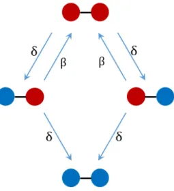
1.1 The Markov process for the network state in the SIS spreading process for a network of two nodes. Red and blue color represent infectious and susceptible state, respectively. β and δ are infection and recovery rates. . . 7
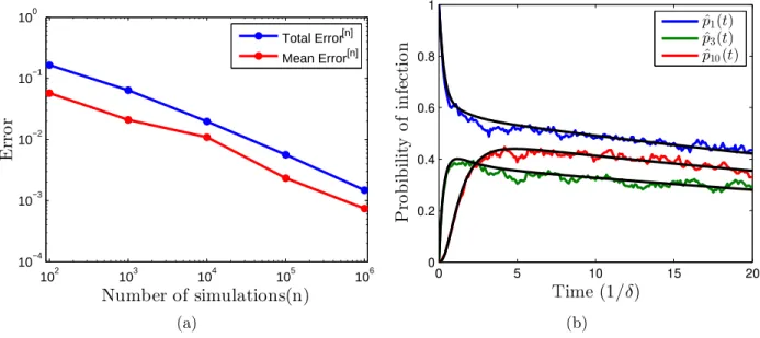
2.1 The infection probability for each node in a toy network of ten nodes estimated using simulation in comparison to the exact probability obtained by solving the Kolmogorov equations for the SIS model: (a) total error and mean error defined in Eqs. (2.1), (2.2), (b) estimation of infection probability for some nodes obtained by averaging over 1000 simulations. The black (smooth) curves are exact probabilities obtained by solving the Kolmogorov equations. . . 17
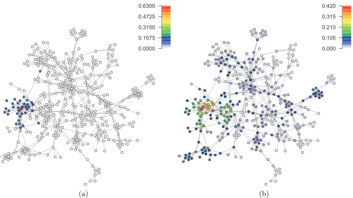
2.2 Result form simulation of SIS spreading over a network. Color of each node represents probability of being infected for the node. (a) probability of being infected at time point t = 0.5 (1/δ), (b) probability at time point t = 90 (1/δ). At t = 0, only the node with the highest degree was infected. These graphs show evolution of infection in the network . . . 18
2.3 Schematic of node-level transitions in the SIR model . . . 18
2.4 Results from 4000 realizations of SIR spreading over a network: (a) histogram of the fraction of removed individuals (b) histogram of extinction time defined as the time when the last infected node in the network is removed . . . 20
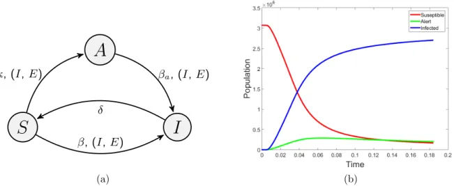
2.5 (a) Schematic of node-level transitions in the SAIS model (b) Simulation of SAIS spreading over a large-scale network. Plot represents the population of each node state in the network over time. . . 21
2.6 Node-level transitions in the SI1SI2S spreading model over a two-layer
net-work. Layers E1 and E2 define two types of contact over the same set of
nodes. . . 22
2.7 Fraction of nodes infected by virus type 2 (above) and virus type 1 (below) in the SI1SI2S competitive spreading model. The infection strength of I2, τ2,
was 5/λ1(B), while the infection strength ofI1,τ1, varied. If 2/λ1(A)≤τ1 ≤
5/λ1(A), viruses coexist; only one virus survives outside this region. . . 23
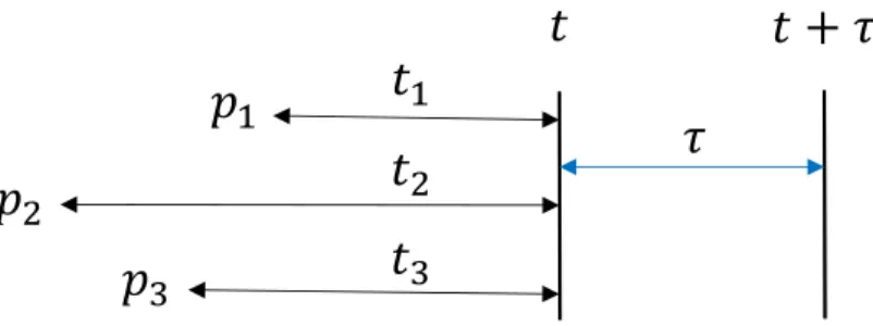
2.8 Three different processes, p1, p2, p3, have been initiated but they have not
occurred up to time t. We want to calculate the probability densities that they occur later at some time denoted by t+τ. . . 24
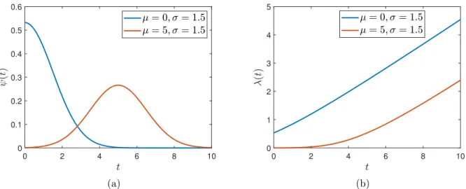
2.9 Panel (a) shows distribution in the equation 2.9 for two different sets of the distribution parameters, and panel(b)shows the corresponding instantaneous rates . . . 28
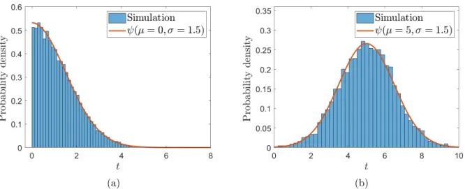
2.10 panels (a) and (b) compare the distribution of transition time in the simulation performed using the approximate non-Markovian algorithm with their exact truncated normal distribution. . . 29
2.11 An example of non-Markovian networked spreading discussed in section 2.3.1 30
2.12 (a) Empirical distributions of the infectious period from reference1. These
curves are clearly non-exponential; (b) Our simulations of the spreading pro-cess obtained using the empirical distributions of figure 2.12.a (upper panel) and using exponential distributions (lower panel) with similar means as the empirical distributions. Fig. 2.12.b shows two sets of epidemic curves, in-fected undetected (exposed and infectious) and confirmed (removed) for the empirical and exponential distributions. Even though the two distributions share the same mean, they have different quantitative behaviors. . . 32
2.13 Non-Markovian simulation of the SEIR model over a population of 60,000 nodes for three different values of the infection transmission rates. For the infectious period we used the distributions in figure2.12.a and we switched to the distribution with the smaller mean at day 57, while keeping the infection transmission rate constant. We can see that panel (b) shows a better fitting of the number of reported cases in Wuhan, China, compared with panels a and c. . . 33
3.1 In this network, we know the link ab exists, but the links bc and ac are uncertain. Also, we know the expected time for transmission of infection through any link is α. Since the difference between the infection time of nodesbandcequals the expected transmission timeαand the same difference calculated for the nodesa and cis 2α, linkbc is expected to be present in the network with a higher probability than linkac. . . 35
3.2 Network used in section 3.4.1. In this network, the link (1,2) exists, but the links (1,4), (2,4), (1,3) and (2,3) are uncertain. Moreover, we assume the transmission rates are symmetric. . . 44
3.3 Plots for the experiment in the section (3.5.1). (a) node degree distribution of the underlying scale-free network. (b) proportion of the infected and sus-ceptible nodes in the SIS trace. (c) distribution of the posterior probabilities for the actual links of the network and (c) distribution of posterior probabil-ities for the non-edge pairs, when different prior distributions and traces of different length were used in the link inference. . . 46
3.4 Results of the experiment in section 3.5.2. (a) and (b) show distributions of the maximum likelihood estimation of the transmission rates for the actual links and the non-edge pairs respectively. (c) and (d) show distributions of the posterior probabilities for the actual links and the non-edge pairs. In the plots, the curves with different T are obtained using SIS traces with different length. . . 49
3.5 Plots show the number of recovered actual links compared to the falsely re-covered non-edge pairs when we apply the thresholding procedure explained in section (3.5.2). The curves are generated by changing the threshold value. To obtain each point on the curves denoted by ”MLE”, we associate a link for any pair of nodes if the MLE of transmission rate between them is higher than the threshold. For the curves denoted by ”Bayesian” we apply threshold on the posterior probabilities. Plots (a), (b), (c), (d) are the result of applying SIS traces of length T ≈ 150, T ≈ 300, T ≈ 450, T ≈ 600 , respectively. In plot (b), λthreshold and Pthreshold are the transmission rate and the posterior
probability thresholds that are applied to obtain the specified point on the curves. . . 55
3.6 Plots for the experiment in the section (3.5.3). (a) node degree distribution of the three different underlying network used in the experiment. (b) propor-tion of the infected nodes in the simulated SIS process over the underlying networks. (c) ,(d) average error, Eq.(3.18), in the inference of the actual links and the non-edge pairs, respectively. . . 56
4.1 A snapshot from a realization of the network model. At any timet the nodes are either active or inactive. A potential link is activated with probabilityp0
4.2 Different processes that result in link establishment between nodes i, j while node i is active. The values in red are the probabilities for each step in the process. . . 62
4.3 Distribution of number of developed links (a) and their duration (b), during the period a node is active. The relevant model parameters are shown in panel (a). . . 63
4.4 The figures show the diagrams of node transitions among different node states. The rate of each transition is specified on the arrow that indicates the transi-tion. (a) shows a diagram of the Markov process which is discussed in section
4.2.2, and (b) shows diagram of the exact process. In these figures I1j = 1 (I2j = 1) if node j is infected and inactive (active), otherwise it is zero. In diagram (b)X0i,j is a Bernoulli random variable that has value one with prob-ability p0. This random variable is drawn each time a pair of active nodes
(i, j) with a potential link between them occurs, regardless of their disease status. . . 66
4.5 Critical value ofβas a function ofγ1 in regular random networks. Parameters:
k1 = 4, k2 = 50, p0 = 0.1, δ= 1, γ2 =γ1 (p2 = 0.5). . . 70
4.6 Disease prevalence as a function of p2 in regular random networks. Circles
show, for each set of parameters values, the median of the prevalence . . . . 70
4.7 Results of numerical and stochastic simulations of the spreading processes on random regular graphs, discussed in section4.4. Panel (a) shows the compari-son of different approximate processes with the exact process; panel (b) shows the epidemic threshold of the exact process, as a function ofp2 (probability of
being active inL2) and the parameter γ2, which is proportional to the inverse
of expected duration of active potential links; panel (c) shows how the infec-tion prevalence in the metastable state is affected by different parameters in the exact process. Error bars show the median and the interquartile range. . 76
4.8 Infection transmission rate threshold as a function of the recovery rate for three different temporal networks discussed in section. Case acorresponds to partnerships of 60 days duration and cases b, c correspond to casual sexual encounters. . . 79
5.1 The Line-Clique graph consisting of a complete graph of size m and a line graph of size N >> m. It is possible to observe a metastable state where infections mostly localize on the clique part — a tiny portion of the network. 83
5.2 (a) The entropy of the optimized distribution for the Line-Clique graph in Fig. 5.1. As can be seen, there is a sudden jump at τ = 12. (b) Monte Carlo simulation of the SIS model over the Line-Clique graph. Color represents dispersion entropy of infection probability distribution divided by ln(N). . . 87
5.3 (a) Optimized probability distribution for β/δ = 0.125, showing only a few localized sites of the network have active nodes (b) Optimized probability distribution forβ/δ = 0.23. . . 87
5.4 (a) The entropy of the optimized distribution normalized by ln(N) for coau-thorships network of Fig. 5.3. (b) Monte Carlo simulation for the SIS where all the nodes were initially infected. Color represents dispersion entropy of the infection probability distribution divided by ln(N) . . . 89
6.1 An example of feedforward neural network . . . 94
6.2 The plots compare the estimated values of the infection prevalence, I(n), with their true values. For plots (a) and (b), we used the energy minimization method for the estimation and used 20 and 50 percent of the nodes, respec-tively, for training. Plots (c) and (d) show the estimation result when we used the radial basis function and the feedforward neural network methods, respectively. In plots (c), (d) we used 20 percent of the nodes for training. . 96
Acknowledgments
I would like to express my gratitude to Dr. Caterina Scoglio for all her supports during my research. I appreciate all the opportunities and helps she provided for me.
I want to thank Dr. Faryad Darabi Sahneh who helped me start doing research in the field of spreading processes. I would also like to thank my committee members, Dr. Pietro Poggi-Corradini, Dr. Nathan Albin, and Dr. Don Gruenbacher for the guidance and comments to improve this dissertation. I also thank Dr. Arslan Munir who accepted to serve as chairperson of the examining committee for my doctoral degree.
Preface
This dissertation with title “Stochastic spreading prepossess on network” is submitted for the degree of Doctor of Philosophy in the Department of Electrical and Computer Engi-neering at Kansas State University. The research has been performed under the supervision of Prof. Caterina Scoglio. Some chapters in the dissertation are adopted from our published peer-reviewed articles:
Vajdi, Aram, David Juher, Joan Salda˜na, and Caterina Scoglio. “A multilayer tempo-ral network model for STD spreading accounting for permanent and casual partners.” Scientific reports 10, no. 1 (2020): 1-12.
Vajdi, Aram, and Caterina M. Scoglio. “Identification of missing links using susceptible-infected-susceptible spreading traces.” IEEE Transactions on Network Science and En-gineering 6, no. 4 (2018): 917-927.
Sahneh, Faryad Darabi, Aram Vajdi, and Caterina Scoglio. “Delocalized epidemics on graphs: A maximum entropy approach.” In 2016 American Control Conference (ACC), pp. 7346-7351. IEEE, 2016.
Sahneh, Faryad Darabi, Aram Vajdi, Heman Shakeri, Futing Fan, and Caterina Scoglio. “GEMFsim: A stochastic simulator for the generalized epidemic modeling framework.” Journal of computational science 22 (2017): 36-44.
Sahneh, Faryad Darabi, Aram Vajdi, Joshua Melander, and Caterina M. Scoglio.“Contact adaption during epidemics: A multilayer network formulation approach.” IEEE Trans-actions on Network Science and Engineering 6, no. 1 (2017): 16-30.
Chapter 1
Introduction
1.1
Stochastic Spreading Processes Over Networks
Spreading processes appear in diverse natural and technological systems. Examples of such processes are the spread of infectious diseases in biological systems, dissemination of infor-mation and ideas in human populations and social networks, and the propagation of malware and fault in technological networks. To understand, predict, and control spreading processes, researchers rely on mathematical models that aspire to describe the underlying mechanisms of their propagation2–8. In simple spreading models, the structure of interactions among indi-viduals is ignored, and a population is categorized into different subpopulations that reflect the nature of the spreading process. For instance, classical epidemiological models3;9 de-fine states (or compartment) such as immune, susceptible, exposed,infectious, symptomatic, recovered, dead, vaccinated, and determine rules for moving individuals from one state to another, assuming the entire population is fully mixed.
During the past two decades, it has been demonstrated that the structure of interaction among population members can dramatically influence the spreading dynamics10–15. There-fore, researchers have focused on studying spreading processes over complex networks where interaction among individuals could be highly heterogeneous16–22. The motivation for such studies is rooted in the complexity of modern societies and the advent of new technologies
that have created complex interconnected systems.
Many types of dynamics can be conceptualized over a complex network23, such as ran-dom walks, diffusion24 , synchronization25, influence propagation26, complex contagion27. Among them, stochastic spreading processes over networks17;18 have drawn substantial at-tention from researchers of different backgrounds. In such a model, the network’s nodes represent entities that can assume various states, and the network’s links represent inter-actions among the nodes that induce the transition of nodes between states. Specifically, stochastic spreading processes over networks are effective when the description of the process at the node level includes some uncertainty, which can be described using such models. For instance, in a biological network, the infection transmission time from an infectious node to a healthy neighbor is a random variable whose distribution can depend on the disease and behavior of individuals. Indeed, one of the main motivations for conducting research on stochastic networked spreading process is to understand and control the collective behavior, even though there are different sources of uncertainty at the individual node level. For ex-ample, analysis of the stochastic susceptible-infected-susceptible (SIS) model over complex networks has clarified the role of the network structure in the emergence of the endemic state, which in turn provides means to control the epidemic by altering the network structure or adopting other possible measures18. The obvious real-world instance of stochastic spreading process is the study of infectious disease transmission. However, such a modeling framework can be applied to study viral information dissemination among users of online social net-works, the propagation of malware or fault in technological netnet-works, or any other stochastic spreading process that can happen in a networked system as a result of interactions among its agents.
Although extensive studies have been conducted over the topic of stochastic networked spreading process, there are various topics in this field that needs to be explored. In this dissertation, we aim to improve our understanding of 1) spreading processes over temporal networks, 2) identification of interaction from node’s states transitions, 3) epidemic localiza-tion, and 4) interpolation of networked spreading data.
1.2
Research Questions
Some of the standard networked spreading models include SI, SIS, SIR and SEIR, where S (Susceptible), E (Exposed), I (Infectious) and R (Recovered) denote the node states. Although these models have different transition rules and node states, at a theoretical level, they can be described using a common framework19. In this dissertation, we study several
aspects of the SIS model, yet some of our methods can be applied to the other stochastic models.
A theoretical question we aim to answer in this dissertation is the possibility of infer-ring unknown network links from observed Susceptible-Infected-Susceptible (SIS) temporal traces. We know that the underlying network affects the epidemic course, and the states that nodes assume through time. For this study, we assume a setting where we observe the transitions of nodes among the two states S and I through time. Using such observations, we want to find the probabilities for the existence of links among different nodes. Such links represent hidden interactions among the nodes.
Another aspect of the SIS spreading, which we explore in this dissertation, is the effect of links’ duration in temporal networks over the spreading of infection. This study is par-ticularly relevant in the context of sexually transmitted diseases (STD) spreading. Recent findings have stressed the increasing role of casual partnerships in STDs spreading and we aim to quantify the effect of such temporal links by analyzing the SIS spreading over a temporal network model that captures casual partnerships.
The third aspect of the SIS model we study in this dissertation is epidemic localiza-tion. The SIS epidemic process on complex networks can show metastability, resembling an endemic equilibrium. In a general setting, the metastable state can either involve a large portion of the network, or be localized on small subgraphs of the contact network. Here, we aim to quantify the localization of an epidemic and calculate its size for a given underlying network and transmission parameters.
In our final study we investigate the interpolation of stochastic networked spreading data. For an SIS spreading or any other type of spreading, various spreading-related functions can
be defined over the network nodes. In this study, we want to explore the possibility of estimating such functions assuming access to the value of these functions over a subset of the nodes.
1.2.1
Contributions
Below is a summary of the main contributions of this dissertation:
1. We developed a software tool capable of simulating a broad range of stochastic spread-ing models with arbitrary transition time distribution(chapter 2).
2. We derived the likelihood of observed SIS temporal traces and inferred the probabilities for the existence of uncertain links. (chapter 3).
3. We developed a time dependent network model appropriate for studying STDs spread-ing and derived the epidemic threshold for the SIS spreadspread-ing over such a network (chapter 4).
4. We proposed a dispersion entropy measure to quantify the localization of infections in a generic contact graph and formulated a maximum entropy problem to find an upper bound for the dispersion entropy of the possible metastable state in the SIS process (chapter 5).
5. We developed a new approach that relies on the effective resistance distance and feed-forward neural network to interpolate spreading data (chapter 6).
1.3
Dissertation Organization
The dissertation is organized as follows. In the rest of this chapter, we introduce the SIS process and discuss the exact and approximate equations that govern the process dynamics. In chapter 2, we explain the computational methods for simulating spreading processes in general. We introduce the software we developed for simulation of networked spreading
processes, and explain the application of such software. In chapter 3, we first derive the likelihood of observing an SIS trace, and we proceed by formulating a Bayesian inference problem that uses the likelihood of observed traces to infer the existence of uncertain links. Later, in that chapter we perform numerical experiments to validate the proposed Bayesian method. In chapter4, we first develop a temporal network model and discuss its implication. Later, we develop a meanfield approximation that describes the SIS spreading over such a network. By analyzing the meanfield equations, we study the effect of the temporal network link durations over the SIS spreading. In chapter 5, the phenomenon of localized epidemics in SIS processes is explored. We propose entropy as a measure of epidemic localization and find an upperbound for this measure. Chapter 6 is devoted to the interpolation methods for spreading data. In that chapter, we proposed a method that uses the effective resistance distance as a measure of similarity between the nodes to estimate the unknown spreading data.
1.4
Background: Networked SIS Spreading
In this section we explain the Susceptible-Infected-Susceptible (SIS) model of networked spreading. By discussing this model we explain important concepts for stochastic spreading processes over networks.
In the SIS model, the population is represented by a network of N nodes G = {V, E}, whereV is the set of nodes and E ⊆V ×V denotes the set of edges between the nodes. An edge represents possible means of infection transmission between the nodes. For the contact network, the adjacency matrixA = [aij]∈RN×N is defined with the elements aij = 1 if and
only if (i, j)∈E else aij = 0.
SIS model assumes the state of node i at time t, denoted by xi(t), is a random variable and xi(t) = 0 if node i is susceptible or xi(t) = 1 if it is infected. A susceptible node becomes infected through interaction with infected neighbors in the network. Moreover, an infected node recovers by itself after some time, and becomes susceptible again. We assume the infection processes are independent. In other words, if two nodes are trying to infect a
common neighbor, the two nodes act independently from each other and the susceptible node becomes infected by the first neighbor that successfully transmits the infection. In general, the transition time from the infected state to the susceptible state is a random variable that can have any distribution. In the same manner, the infectious time is a random variable.
In the Markovian SIS model, the recovery time for an infected node is exponentially distributed with a curing rate δ ∈ R+. In other words, if a node is infected the probability
for that node to stay infected, exponentially decreases with time. Similarly, if a susceptible node is in contact with an infected node, the probability to stay susceptible exponentially decreases with time by the infection rateβ ∈R+. If a susceptible node is in contact with more
than one infected neighbor, the infection occurs at rateβyi(t), whereyi(t),PN
j=1aijxj(t) is
the number of infected neighbors. The exact mathematical treatment of the Markovian SIS process requires considering the joint state of all the nodes X,[x1, ..., xN], in other words,
the network state. Indeed, the network state defines a continuous-time Markov process over a space consisting of 2N possible states. Figure 1.1, shows the Markov process and the transitions for a network of two nodes. In this figure, we can see the absorbing state of the Markov process is the state where both nodes are susceptible. For a network with a small number of nodes, it is possible to write the Kolmogorov equations for the Markov process resulting from the SIS process. However, when the number of nodes grows, the number of possible states for the Markov process grows exponentially, i.e., 2N. This hinders the exact mathematical treatment of the SIS process over networks.
To derive the N-intertwined18 approximation for the Markovian SIS process, we can use the following equation obtained from the node-level description of the SIS process
d
dtE[xi] =β
X
aijE[(1−xi)xj]−δE[xi] (1.1)
=βXaijE[xj]−βXaijE[xixj]−δE[xi]
for i ∈ {1, ..., N}. In this equation E(xi) is the expected value for the node state random variablexi. Indeed,E(xi) is probability of finding nodeiinfected and similarly, E[(1−xi)xj] is the joint probability that node i is susceptible and node j is infected. Equation (1.1) is
Figure 1.1: The Markov process for the network state in the SIS spreading process for a net-work of two nodes. Red and blue color represent infectious and susceptible state, respectively.
β and δ are infection and recovery rates.
not a closed system as the evolution of E[xi] depends on the joint probabilities of the pairs
xixj. Furthermore, if we proceed to derive the time derivative of E[xixj], it turns out the time derivative depends on the higher order terms E[xixjxk] which are the expected values of the triplets. The procedure goes on until we reach a closed system of 2N −1 equations
involvingE[xi...xN]. Such exponentially enormous state space of the exact model challenges the feasibility of any analytical investigation of the exact SIS process.
To derive approximated results, researchers use the mean-field approximation where the termE[xixj] in equation (1.1) is approximated by the multiplication of marginal probabilities
E[xi]E[xj]18;28. By applying this approximation equation (1.1) can be rewritten as
d
dtE[xi] =β
X
aijE[(1−xi)]E[xj]−δE[xi] (1.2)
Equation (1.2) and similar types of approximate equations have been the starting points in analyzing networked spreading processes18;29;30. For example, by analyzing equation (1.2), it
is shown forβ/δ < λ−1
A, the prevalence of infection PN
i=1E[xi] in the SIS process dies out exponentially fast
18.
This result has motivated research papers on the optimization of the largest eigenvalue of adjacency matrices to control the SIS spreading process31;32. Finally we want to emphasize two important facts about the N-intertwined mean-field equations. First, these equations are only relevant to Markovian processes. Second, they provide an upper-bound for the nodal infection probabilities28.
Chapter 2
Simulation of Stochastic Spreading
Processes
1
2.1
Introduction
In general, the exact mathematical treatment of stochastic networked spreading process is not tractable, even for the simplest spreading models and a small number of nodes in the network. This problem stems from the fact that in the exact analysis we need to consider the network state, in other words, the state of all the nodes concurrently, instead of each node’s state independently. Therefore, we have developed a software tool that can simulate the exact stochastic process for a broad range of networked spreading models.
In this chapter, we introduce two computational tools that can numerically simulate a broad range of spreading processes over complex networks. These two tools are based on the Gillespie algorithm34;35, and a modified Gillespie algorithm36. The Gillespie algorithm gener-ates statistically correct trajectories of continuous-time Markov processes while the modified Gillespie algorithm is an approximate method for simulating non-Markovian processes.
Indeed, the number of possible spreading models that can be defined is limitless because the possible node states and node state transitions are not restricted. However, most
worked spreading processes share a common fundamental assumption: nodes influence each other through independent pairwise interactions. Independent means that different nodes in the network influence a common neighbor through statistically independent processes. Pair-wise indicates that no higher order interaction is permitted, i.e., joint interaction of three nodes A–B–C is fully described by A–B, B–C, and A–C interactions.
Based on the independent pairwise interaction characteristic of most spreading models, Sahnehet al.19defined the generalized epidemic modeling framework (GEMF) that incorpo-rates a broad spectrum of stochastic spreading processes over complex networks. In order to make our computational tools applicable to a broad range of spreading models, we chose to implement the Gillespie algorithm and the modified Gillespie algorithm for the generalized epidemic modeling framework.
2.1.1
Generalized Epidemic Modeling Framework
GEMF describes a general epidemic model over a network composed of one set of nodes and several layers of contact. We represent the network by G(V, E1,· · ·, EL), where L is the
number of contact layers,V is a set ofN nodes, andElis a set of links between the nodes in layer l. The incorporation of multilayer typologies in GEMF makes it a flexible framework for studying epidemic processes.
Similar to the SIS model, state of noden at timet is a random variable denoted byxn(t) and each node can assume a node state among M possible states, which are labeled with an integer from 1 to M, i.e., xn(t) ∈ {1,· · · , M}. In GEMF, transitions of xn over the node states are classified into two categories.
1. Nodal transitions of a node are similar to the curing process in the SIS model and they are independent of the neighbors’ state.
2. Edge-based transitions of a node are analogous to the infecting process in the SIS model. These transitions are caused by the interaction of a node with its neighbors in the network, and they depend on states of the neighbors. In GEMF each network layer has its own influencer state. If a node is in an influencer state of a layer it will induce
some transitions on its neighbors in that network layer. For instance, the influencer state in the SIS model is the infected state. The network layer provides contacts for a node in the influencer state to induce and propagate certain transitions over neighboring nodes.
2.2
Simulation of Markovian Processes
The Gillespie algorithm is a method for sampling the earliest event among a set of inde-pendent events assuming the occurring time for each event is exponentially distributed. To understand the Gillespie algorithm, consider a set of k independent nodes where each node, such as noden, will make a transition from stateito statej at a random timeTn∼exp(rn). This random time Tn has an exponential distribution with rate rn. In this case, since the transition of a node does not affect the transition of other nodes, we can generate the tran-sition time for each node by drawing a random value from its corresponding distribution. If we arrange these transition times in increasing order we get a sequence of events. The Gillespie algorithm is another method that generates such sequences of events. It starts with all ongoing processes and samples the time for the earliest event and the node that makes the transition. Next, the algorithm advances the time and repeat the same procedure for the remaining processes. Although the Gillespie algorithm can be applied to the case of k
independent nodes we described above, it is more applicable in simulating the Markovian dynamics of a complex system where the occurrence of an event can affect other ongoing processes in the system. For instance, consider an infection process of a node by two infected neighbors. In this case the infected neighbors can infect the target node through indepen-dent processes. However, when an infection event happens the competing infection process is assumed to be terminated. In order to sample the time for the infection of the target node, we can generate two random times and accept the shortest time as the infection time. When we use the Gillespie algorithm we can generate the infection time directly. Indeed, the Gillespie algorithm relies on the fact that the minimum of exponentially distributed in-dependent random variables has an exponential distribution with a rate equal to the sum of the individual rates37. Hence, we only need to generate one random infection time from an
exponential distribution whose rate is the sum of the competing infection processes’ rates.
2.2.1
Algorithm
Considering the node-level description of transitions in GEMF, the node transition xn → j
may be viable through different possible processes. In other words, node n may undergo a transition from its current state xn to any state j by interacting with neighbors or through a nodal transition. In such a case, the processes are assumed to be competing independent processes that try to induce the transition xn → j. Thus, the actual transition time of node n, Txn→j, is the minimum of transition times for the competing processes, Txn→j = min{T1,· · · , Tp}. If the transition times in all the independent processes are distributed
exponentially, T1 ∼ exp(r1),· · · , Tk ∼ exp(rp), distribution of the transition time Txn→j is exponential with a rate which is sum of all rates for the possible processes, i.e., Txn→j ∼ exp(λn(xn →j)) where λn(xn→j) = P
prp.
To proceed with the simulation algorithm, we define two arrays:
Nodal transition matrix, Aδ, where the element Aδ(i, j) is the transition rate of a node from state i to statej via a nodal transition.
Edge based transition array, Aβ, where the element Aβ(i, j;l) is the transition rate for the transition of a target node from state i toj through an interaction with a neighbor in layer l while the neighbor is in state q(l). Stateq(l) is the influencer state for layer l.
In fact, the elements of Aδ and Aβ define the rates for the exponential distribution of transition times corresponding to the possible processes allowed in GEMF. If a rate is zero the corresponding transition never happens.
Assuming the joint state of the network at time t is X(t) = [x1,· · · , xN], we can
calcu-late all node-level transition rates λn(xn → j), for any node n, using the nodal transition matrixAδ, edge-based transition array Aβ and the contact networkG(V, E1,· · · , EL), where
λn(xn→j) is the transition rate of node n from its current state xn to the state j.
However, the occurrence of any node-level transition can affect other ongoing processes in the network. Hence, we will follow the Gillespie algorithm and sample the earliest transition.
If we define S as the set of all node-level transition times
S ={Tn(xn→j)|n ∈ {1,· · ·, N}, j ∈ {1,· · · , M}},
the elements of S are independent exponentially distributed random variables. Using the theorem concerning the minimum of independent exponential distributions37, then the
probability that Tn(xn →j) would be the minimum of S is
Pr (Tn(xn→j) = min(S)) = λn(xn →j)
λtot ,
where λtot ,P
n
P
jλn(xn →j). Using this probability distribution, we can sample one of
the node-level transitions. We also must sample the time at which this transition occurs. Because elements of S have exponential distributions, if we define T = min(S), then T
is exponentially distributed with a rate equal to λtot. Thus, using the distribution of T, we sample a time for the network state transition. The memoryless property of Markov processes allows the entire described procedure to be repeated after the network state is updated. Particularly, we can directly update the transition rates by the adjustment required due to the change in the state of node n that made the transition, including updating the transition rates of node n and neighbors that can be affected by node n. The other rates remain constant.
The described simulation method is summarized in Algorithm 1, where we assume that network links can be directed and weighted. If a link is directed from node m to node n, nodem can induce edge-based transitions on node n, but node n cannot induce edge-based transitions on nodem. Moreover, we can assign a weight to each link in order to quantify the effect of neighbors on edge-based transitions of a node. The rate of an edge-based transition induced by a link is multiplied by the weight of the link. In Algorithm 1, W(m, n;l) is the weight of the link directed from nodemto nodenin layerlof the network, andW(m, n;l) = 0 indicates that such a link does not exist. However, implementation of Algorithm 1 requires to only store the nonzero weights. In Algorithm1, input q(l) is the influencer node state for
Algorithm 1 GEMFsim algorithm
Input Aδ,Aβ, W, X0, q, Stop condition
Output: event 1: X ←X0 2: for n = 1 to N do 3: for l= 1 to L do 4: wq(n, l)← N P m=1 W(m, n;l)δxm,q(l) 5: end for 6: λn ← M P j=1 Aδ(xn, j) + L P l=1 wq(n, l)Aβ(xn, j;l) 7: end for 8: λtot ← N P n=1 λn 9: k = 0
10: while Stop condition=FALSEdo
11: α∼Unif(0,1) . generate α from Unif(0,1)
12: δtk ← −log(α)/λtot . time period to the next event 13: P1(n)←λn/λtot
14: nk∼P1 . sample nk from probability distribution P1
15: ik ←xnk 16: for j = 1 to M do 17: λnk(ik →j)←Aδ(ik, j) + L P l=1 wq(nk, l)Aβ(ik, j;l) 18: end for 19: P2(j)←λnk(ik→j)/λnk
20: fk ∼P2 . samplefk from distribution P2
21: event(k)←(δtk, nk, fk, ik)
22: xnk ←fk . update network state
23: for l | (q(l) =fk or q(l) = ik) do .Update Rates
24: ∆←δq(l),fk −δq(l),ik 25: for n | W(nk, n;l)6= 0 do 26: wq(n, l)←wq(n, l) + ∆×W(nk, n;l) 27: λn←λn+ ∆× M P j=1 W(nk, n;l)Aβ(xn, j;l) 28: end for 29: end for 30: λnk ← M P j=1 Aδ(fk, j) + L P l=1 wq(nk, l)Aβ(fk, j;l) 31: λtot ← N P n=1 λn
32: Update Stop condition
33: k ←k+ 1
layer l, Aδ and Aβ are nodal transition rates and edge-based transition rates, respectively, and X0 is the initial network state. Assuming the current network state X = [x1,· · · , xn],
node-level transition rates are calculated as
λn(xn →j) =Aδ(xn, j) + L X l=1 Aβ(xn, j;l) N X m=1 W(m, n;l)δxm,q(l),
whereδs,tis Kronecker delta. In Algorithm1, we sample a node-level transition in three steps. First, we generate one sample for a random variable δt which is exponentially distributed with the rate λtot. In fact, δt is the time period between the network state events, and
λtot = PN
n=1λn, where λn =
PM
j=1λn(xn → j). Generating a sample for δt is done by
generating a sample α from the uniform distribution over the interval (0,1), and inserting
α into the equation δt = −log(α)/λtot. The second step is to select a node according to the probability distribution Pr(n) =λn/λtot. This is the node that will make the transition. After the node is picked, we select a new node statejfor the node according to the probability distribution Pr(j | n) = λn(xn → j)/λn. The event-based algorithm explained above is an adaptation of the Gillespie algorithm34;35, to GEMF-based processes. Implementation of the algorithm is available online38.
2.2.2
Simulations
A broad spectrum of epidemic models can be formulated in the GEMF framework. Hence, the algorithm we described above is a flexible platform capable of simulating various stochastic spreading models.Here, we show how GEMFsim (implementation of Algorithm 1) can be applied to study various compartment models that fit the description of GEMF processes. GEMFsim provides realizations of Markov processes over a space consisting of network states. In theory, GEMFsim can be used to generate enough samples to extract statistics of interest. In fact, any statistics defined in terms of marginal distributions of the Markov processes can be estimated using samples generated by the GEMFsim tool.
Comparison to Exact Kolmogorov Equations
The sampled network state trajectories generated using algorithm 1 follow a distribution which is the solution of the Kolmogorov equations for the Markov process governing the network state evolution. To experimentally test the distribution of the generated samples, we compared results of the simulation with the exact solution of the Kolmogorov equations for the SIS model. The Kolmogorov equations for the SIS process over a network ofN nodes is a linear system of 2N coupled equations and the size of linear system becomes gigantic, even
for moderate values of N. Therefore, we considered a small network of N = 10 nodes with SIS parameters ofδ= 1 andβ = 2. Assuming an initial condition in which only one node was infected, we solved the Kolmogorov equations, ˙P(t) = −QTP(t)19, whereP is a probability
distribution over a space consisting of 210 = 1,024 network states and Q is the infinitesimal
generator matrix. We then extracted the infection probability of each node, pexact
i (t), as a
marginal distribution of P(t). Next, using Algorithm 1, we generated n realizations of the SIS process and obtained an estimation for the infection probability of nodei, ˆp[in](t), as the fraction of realizations that node i was infected at time t. Our objective was to observe if the difference between ˆp[in](t) andpexact
i (t) decreases as the number of realizationn increases.
Therefore, we defined two measures of error as
Total Error[n],max
i maxt |pˆ
[n]
i (t)−p exact
i (t)|, (2.1)
Mean Error[n],max
t 1 N| N X i=1 ˆ p[in](t)−pexact i (t)|. (2.2)
Fig. (2.1a) shows how the defined measures decreased when the number of realization n
increased.
Simulation of the SIS Model
The SIS model is one of the simplest models that can be simulated using GEMFsim. In this model each node is either susceptible (S) or infected (I), as represented by the integers 1 or 2, respectively. If a node is infected, it transmits infection to the susceptible neighbors at a rate
102 103 104 105 106 10−4 10−3 10−2 10−1 100 E rr o r Number of simulations(n) Total Error[n] Mean Error[n] (a) 0 5 10 15 20 0 0.2 0.4 0.6 0.8 1 Time (1/δ) P ro b ib il it y o f in fe ct io n ˆ p1(t) ˆ p3(t) ˆ p10(t) (b)
Figure 2.1: The infection probability for each node in a toy network of ten nodes estimated using simulation in comparison to the exact probability obtained by solving the Kolmogorov equations for the SIS model: (a) total error and mean error defined in Eqs. (2.1), (2.2), (b) estimation of infection probability for some nodes obtained by averaging over 1000 simula-tions. The black (smooth) curves are exact probabilities obtained by solving the Kolmogorov equations.
β, and the infected node recovers with the rateδ. We simulated SIS spreading over a contact network consisting of one layer of contact G(V, E). The network we used was the largest component of the coauthorship network presented in39. We assumed that the links were
undirected and had identical weight. Based on description of the nodal transition matrix,
Aδ, and the edge-based transition array,Aβ, the nonzero elements of them in the SIS model are Aδ(2,1) = δ and Aβ(1,2; 1) = β. Moreover, the influencer node state for this model is the infected state, i.e., q(1) = 2. Using the implementation of GEMFsim algorithm in R38
we generated 8000 realizations of SIS spreading. We used the results of these simulations to estimate the probability of being infected for each node in the network at various time points. The probability of being infected was estimated as the fraction of SIS realizations in which the node was infected at the given time point. Results for two time points are plotted in Fig. (2.2). We assumed β = 0.23 and δ= 1. The only node that was initially infected in all realizations was the node with the highest degree.
● ● ● ● ● ● ● ● ● ● ● ● ● ● ● ● ● ● ● ● ● ●● ● ● ● ● ● ● ● ● ● ● ● ● ● ● ● ● ● ● ● ● ● ● ● ● ● ● ● ● ● ● ● ● ● ● ● ● ● ● ● ● ● ● ● ● ● ● ● ● ● ● ● ● ● ● ● ● ● ● ● ● ● ● ●● ● ● ● ● ● ● ● ● ● ● ●● ● ● ● ● ●● ● ● ● ● ● ● ● ● ● ● ● ● ● ● ● ● ● ● ● ● ● ● ● ● ● ● ● ●● ● ● ● ● ● ● ● ● ● ● ● ● ●● ● ● ● ● ● ● ● ● ● ● ● ● ● ● ● ● ● ● ● ● ● ● ● ● ● ● ● ●● ●● ● ● ● ● ● ●●● ● ● ● ● ● ● ● ● ● ● ● ● ● ● ●● ● ● ● ● ● ● ● ● ● ● ● ● ● ● ● ● ● ● ●●● ● ● ● ● ● ● ● ●● ● ● ● ● ● ● ● ● ● ● ● ● ● ● ● ● ● ● ● ● ● ●● ● ● ● ● ● ●● ● ● ● ● ● ● ● ● ● ● ● ● ● ● ● ● ● ● ● ● ● ● ● ● ● ● ● ● ● ● ● ● ● ● ● ● ● ● ● ● ● ● ● ● ● ● ● ● ● ● ● ● ● ● ●● ● ● ● ● ● ● ● ● ● ● ● ● ● ● ● ● ● ● ●● ● ● ● ● ● ● ● ● ● ● ● ● ● ● ● ● ● ● ● ● ● ● ● ● ● ● ● ●● ● ● ● ● ● ● ● ● ● ● ● 0.0000 0.1575 0.3150 0.4725 0.6300 (a) ● ● ● ● ● ● ● ● ● ● ● ● ● ● ● ● ● ● ●● ●●● ● ● ● ● ● ● ● ● ● ● ● ● ● ● ● ● ● ● ● ● ● ● ● ● ● ● ● ● ● ● ● ● ● ● ● ● ● ● ● ● ● ● ● ● ● ● ● ● ● ● ● ● ● ● ● ● ● ● ● ● ● ● ●● ● ● ● ● ● ● ● ● ● ● ●● ● ● ● ● ●● ● ● ● ● ● ● ● ● ● ● ● ● ● ● ● ● ● ● ● ● ● ● ● ● ● ● ● ●● ● ● ● ● ● ● ● ● ● ● ● ● ●● ● ● ● ● ● ● ●● ● ● ● ● ● ● ● ● ● ● ● ● ● ● ● ● ● ●● ●● ●● ● ● ● ● ● ●●● ● ● ● ● ● ● ● ● ● ● ● ● ● ● ●● ● ● ● ● ● ● ● ● ● ● ● ● ● ● ● ● ● ● ●●● ● ● ●● ● ● ● ●● ● ● ● ● ● ● ● ● ● ● ● ● ●● ● ● ● ● ● ● ● ●● ● ● ● ● ● ●● ● ● ● ● ● ● ● ● ● ● ● ● ● ● ● ● ● ● ● ● ● ● ● ● ● ● ● ● ● ● ● ● ● ● ● ● ● ● ● ● ● ● ● ● ● ● ● ● ● ● ● ● ● ● ●● ● ● ● ● ● ● ● ● ● ● ● ● ● ● ● ● ● ● ●● ●● ● ● ● ● ● ● ● ● ● ● ● ● ● ● ● ● ● ● ● ● ● ● ● ● ● ●● ● ● ● ● ● ● ● ● ● ● ● 0.000 0.105 0.210 0.315 0.420 (b)
Figure 2.2: Result form simulation of SIS spreading over a network. Color of each node represents probability of being infected for the node. (a) probability of being infected at time point t= 0.5 (1/δ), (b) probability at time point t = 90 (1/δ). At t= 0, only the node with the highest degree was infected. These graphs show evolution of infection in the network
S
I
R
β, (I, E) δ
Figure 2.3: Schematic of node-level transitions in the SIR model
Simulation of SIR Model
Here we show how GEMFsim can be used to estimate certain statistics which are beyond the scope of mean-field-type approximations. In fact, GEMFsim can be used to generate several realizations of a spreading process and estimate probability distribution for the epidemic measure of interest. We considered an SIR epidemic model in which a susceptible node becomes infected with the rate β as a consequence of interacting with infected neighbors. Moreover, an infected individual makes a transition to a removed state that may represent the recovered immune state. This transition occurs independently of state of neighbors;
in Fig.(2.3), the transition rate is shown by δ. In the SIR model, a removed node does not affect its neighbors or undergo any transition, and the network eventually reaches an absorbing state in which all individuals are susceptible or removed. Although the time at which the network falls into the absorbing state is not a deterministic variable, the simulation can be used to estimate the probability distribution for the extinction time. The final number of removed individuals is an important measure in epidemiology because it shows the size of outbreak. Similar to extinction time, we can use simulation to estimate probability distribution of the total number of individuals removed.
We used GEMFsim in MATLAB to generate 4000 realizations of SIR spreading over a directed and weighted network composed of 1899 nodes and 20296 edges. This network has been studied in reference40, and its dataset is available online with the name of Facebook-like social network40. We assumed initially only one node, which is labeled by integer 1 in the dataset, was infected and the rest of nodes in the network were susceptible. We used transition rates β = 0.05 and δ = 1 for the simulation. Node states in the SIR model are susceptible, infected and removed as labeled by the integers 1, 2, and 3, respectively. The network has one layer of contact with a set of directed and weighted links, and the influencer state is the infected state, represented by integer 2, i.e., q(1) = 2. The only nonzero elements of the nodal transition matrix and the edge based transition array are Aδ(2,3) = δ and
Aβ(1,2; 1) = β. Using simulation we were able to generate a histogram of the extinction time and the total fraction of removed individuals in the defined SIR spreading. Fig. (2.4) shows the total number of affected individuals and extinction time as they follow bimodal distributions.
Simulation of SAIS Model
The Susceptible-Alert-Infected-Susceptible (SAIS) model was developed to incorporate in-dividual reactions to the spread of a virus41;42. In the SAIS spreading model, each node
(individual) is either susceptible (S), infected (I), or susceptible-alert (A). A susceptible node gets infected with a rate β through interaction with an infected node, and an infected
0 0.1 0.2 0.3 0.4 0.5 0 200 400 600 800
Proportion of individuals removed
Nu m b er o f si m u la ti o n s (a) 0 5 10 15 20 0 100 200 300 Extinction time (1/δ) Nu m b er o f si m u la ti o n s (b)
Figure 2.4: Results from 4000 realizations of SIR spreading over a network: (a) histogram of the fraction of removed individuals (b) histogram of extinction time defined as the time when the last infected node in the network is removed
node recovers with a rate δ. The SAIS model also accounts for another possibility that a susceptible node can become alert with a rate κif it senses an infected node in its neighbor-hood. An alert node can also become infected by a process similar to the infection process of a susceptible node. However, the infection rate for an alert node, denoted by βa, is lower due to the adoption of preventative behaviors. In order to simulate a realization of the SAIS process, we set up a problem according to the GEMF framework in which three node states (S, A, I) were denoted by integers 1,2,3, respectively. The network had one layer of contact, G(V, E), where E represents a set of links that could be generally directed and weighted. The influencer state in this model was infected state as represented by integer 3, i.e., q(1) = 3. The only nonzero element of the nodal transition matrix in the SAIS model isAδ(3,1) =δ. The nonzero elements of the edge-based transition array are Aβ(1,3; 1) =β,
Aβ(2,3; 1) =βa, and Aβ(1,2; 1) =κ. Schematic of node-level transitions in the SAIS model is shown in Fig. (2.5a)
Using the implementation of GEMFsim algorithm in C language38 we generated one
A
S
I
βa, (I, E) κ, (I, E) β, (I, E) δ (a) (b)Figure 2.5: (a) Schematic of node-level transitions in the SAIS model (b) Simulation of SAIS spreading over a large-scale network. Plot represents the population of each node state in the network over time.
through 11,7185,083 links. Network links were undirected and had identical weights. The simulation result is shown in Fig. (2.5b). The simulation initially began with 20 infected nodes and 20 nodes in the alert state; the other nodes in the network were initially susceptible. Transition rates for the simulation were δ= 1, β = 2, βa= 0.4, andκ = 0.2.
Simulation of SI1SI2S Model
The SI1SI2S model is an extension of the SIS model in which two types of infection can attack
a susceptible node29. However, we assumed a competitive scenario in which the two viruses were exclusive, or a node did not harbor both types of infection simultaneously. Therefore, in this model, each node is either susceptible (S), infected by virus one (I1), or infected by
virus two (I2). Similar to the SIS model, infected nodes recover with a rateδ1orδ2depending
on the infection. In general, different infections can be transmitted to a susceptible node through different contacts. In order to account for different means of spreading for I1 and
I2, the assumption was made that they spread through different layers of contact such that
a susceptible node undergoes a transition to infected stateI1 (I2) with a rate β1 (β2) if it is
in contact with anI1 (I2) node through layerE1 (E2). Fig. (2.6) depicts the SI1SI2S model
S
I
1I
2 β2, (I2,E2) β1, (I1,E1) δ1 δ2 Layer E1 Layer E2Figure 2.6: Node-level transitions in the SI1SI2S spreading model over a two-layer network.
Layers E1 and E2 define two types of contact over the same set of nodes.
states (S, I1, I2) represented by integers 1,2,3, respectively. The network consists of two
layers, G(V, E1, E2), where the first layer spreadsI1, and the second layer,I2. The influencer
node state for layer one isI1and the influencer node state for the second layer isI2. The only
nonzero elements of nodal transition matrix are Aδ(2,1) = δ1 and Aδ(3,1) = δ2. Nonzero
elements of edge-based transition array areAβ(1,2; 1) =β1 andAβ(1,3; 2) =β2. In general,
E1, E2 could be two different sets of links between nodes. However, if both types of infection
use the same kind of contacts to spread, E1 and E2 are similar.
The SI1SI2S model described above, exemplifies a competitive spreading scenario in which
two types of infection try to invade a network. However, mean-field-type approximation shows, in a network with two different layers of contact, I1 and I2 can coexist depending on
their infection rates29. We used the implementation of GEMFsim in Python38 to show this coexistence via simulation. We adopted a network of 500 nodes with two different contact layers, E1 and E2. We assumed I1 spreads through contact layer E1, which is a scale-free
network44 of 2,475 edges and that I2 uses a geometric network, E2, of 3,560 edges to invade
0.0 0.1 0.2 0.3 0.4 0.5 0.6 0.7 0.8 0.9 virus 2 infection fraction 1 2 3 4 5 6 7 λ1(A)τ1 0.0 0.1 0.2 0.3 0.4 0.5 0.6 0.7 0.8 0.9 virus 1 infection fraction
Figure 2.7: Fraction of nodes infected by virus type 2 (above) and virus type 1 (below) in the SI1SI2S competitive spreading model. The infection strength ofI2, τ2, was5/λ1(B), while
the infection strength ofI1, τ1, varied. If 2/λ1(A)≤τ1 ≤5/λ1(A), viruses coexist; only one
virus survives outside this region.
of 5/λ1(B) as the infection strength τ2 = β2/δ2 where λ1(B) is the largest eigenvalue of
adjacency matrix B. However, for infection strength τ1 =β1/δ1 we used seven values from
τ1 = 1/λ1(A) to τ1 = 7/λ1(A); for each value of τ1 we generated 500 realizations of SI1SI2S
processes. For all simulations we assumed that each virus had initially infected 2% of the nodes. Fig. (2.7) shows metastable state population sizes extracted from simulations for values ofτ1. As shown in the figure, either one of the viruses prevails or the viruses coexist
depending on the value ofτ1.
2.3
Simulation of non-Markovian Stochastic Processes
In this section, we discuss a general method that can be used for simulation of independent non-Markovian processes36. Since this method uses the concept of the earliest event, it can
ݐ
ଵݐ
ଶݐ
ଷ
ଵ
ଶ
ଷݐ
ݐ ߬
߬
Figure 2.8: Three different processes, p1, p2, p3, have been initiated but they have not
occurred up to time t. We want to calculate the probability densities that they occur later at some time denoted by t+τ.
be considered a generalized Gillespie algorithm.
Consider a set of N statistically independent processes, each with an inter-event time distribution ψi(τ); i ∈ {1,· · · , N}. Suppose that, for a given process i, we know ti, which is the time interval between the process initiation and the latest observation of the process performed at the current time t (see figure 2.8 for illustration). First, we want to know what is the probability density that the event for process i will happen in the time interval [τ, τ +dτ] where τ is measured from current moment t. This probability density can be written as ψi(τ|ti) = ψi(τ +ti) Ψi(ti) , where Ψi(ti) = R∞
ti ψi(s)ds is the survival function of processiand gives the probability that the event for processidoes not happen in the time interval [0, ti] after the process initiation. Indeed, ψi is the truncated distribution for the inter-event time and reflects our observation that the process has survived up toti from its initiation.
To generate a statistically correct sequence of events for the set of all ongoing processes, in the next step, we should calculate the probability density that the next event corresponds to the process i among all the processes, and it will occur at time τ+ti. This probability is
φ(τ, i|{tk}) =ψi(τ|ti)Y k6=i Ψk(τ|tk) = ψi(τ+ti) Ψi(τ +ti) N Y k=1 Ψk(τ|tk), (2.3)
where Ψi(τ|ti) is the conditional survival probability, Ψi(τ|ti) = Z ∞ τ ψi(s|ti)ds = Ψi(τ+ti) Ψi(ti) ,
which is the probability that the event for the processioccurs aftert+τ, assuming we know it did not happened beforet. To sample a time for the occurrence of next event, we evaluate the joint conditional survival function, which is the probability that no event happens before
t+τ and it can be written as
Φ(τ|{tk}) = N Y k=1 Ψk(τ|tk) = N Y k=1 Ψk(τ+tk) Ψk(tk) . (2.4)
Now we can express the algorithm for the generation of a statistically correct sequence of events as follows:
1. draw u a random number in the interval (0,1) and find the random time for the next event τ by solvingu= Φ(τ|{tk}).
2. choose a process that corresponds to the next event by sampling the following discrete distribution p(i) = Pφ(τ, i|{tk}) jφ(τ, j|{tk}) = Pλi(τ+ti) jλj(τ+tj) ,
where λi(s)≡ψi(s)/Ψi(s) is the instantaneous rate of the process.
3. update the elapsed time for the processes
tk→tk+τ,∀k 6=i and ti = 0;
4. update the processes. Terminate some processes or activate new processes if needed. Go to step 1.
To understand the connection between the algorithm above and the original Gillespie algorithm, assume that all the processes in the algorithm are Markovian, i.e., the transition
times are exponentially distributed, ψk(t) = rkexp(−rkt) for k ∈ {1,· · · , N}. With this assumption, the survival function for any processk becomes exp(−rkt). Therefore, the joint conditional survival function in the equation2.4 can be written as
Φ(τ|{tk}) = N Y k=1 Ψk(τ|tk) = N Y k=1 exp(−rkτ) = exp(−τX k rk). (2.5)
Using this equation, we can see the distribution of the earliest transition time, τ, is expo-nential with the rate equal P
krk. This is the result of the Markovian nature of exponential
distributions, which make the conditional survival functions, Ψk(τ|tk), independent of the
age of processes, tk. Hence, step one in the algorithm for the simulation of non-Markovian processes is the generalization of the step in the Gillespie algorithm where we sample the earliest event for a set of independent Markovian processes. Moreover, the instantaneous rates defined in step 2 of the non-Markovian algorithm reduce to the rates of exponential distributions, λi(s) = ri, which are constant. Therefore, the non-Markovian algorithm fol-lows the same logic as the Gillespie algorithm except that the processes have variable ages, and the rates are not constant.
Although the non-Markovian algorithm is statistically exact, it can be computationally expensive. In step one of the algorithm, we need to solve the equation u = Φ(τ|{tk}), to find the time to the next event, τ. This step can be computationally expensive. However, if we use the following approximation
Ψk(τ +tk)≈Ψk(tk) +τΨ0k(tk) = Ψk(tk)−τ ψk(tk) = Ψk(tk)(1−τ λk(tk)), (2.6)
where we have assumedτ ∼0, the joint conditional distribution can be approximated as Φ(τ|{tk})≈ N Y k=1 (1−τ λk(tk))≈1−τ N X k=1 λk(tk). (2.7)