Robust synthetic control

Robust Synthetic Control

by

Dennis Shen

B.S., University of California San Diego (2015)

MASSACHUSETTS INSTITUTE OF TECHNOLOGY

MAR

2

6 2018

LIBRARIES

ARCHIVES

Submitted to the Department of Electrical Engineering and Computer

Science

in partial fulfillment of the requirements for the degree of

Master of Science

at the

MASSACHUSETTS INSTITUTE OF TECHNOLOGY

February 2018

Massachusetts Institute of Technology 2018. All rights reserved.

A uthor ...

Department of Electrical Engineering and Computer Science

September 28, 2017

C ertified by ...

'

'

Devavrat Shah

Professor of Electrical Engineering and Computer Science

Thesis Supervisor

Accepted by ...

rd

ce

Lddi&-A. Kolodziejski

Professor of Electrical Engineering and Computer Science

Chair, Department Committee on Graduate Students

MITLibraries

77 Massachusetts Avenue

Cambridge, MA 02139 http://Iibraries.mit.edu/ask

DISCLAIMER NOTICE

Due to the condition of the original material, there are unavoidable

flaws in this reproduction. We have made every effort possible to

provide you with the best copy available.

Thank you.

The images contained in this document are of the

best quality available.

Robust Synthetic Control

by

Dennis Shen

Submitted to the Department of Electrical Engineering and Computer Science on September 28, 2017, in partial fulfillment of the

requirements for the degree of Master of Science

Abstract

In this thesis, we present a robust generalization of the synthetic control method.

A distinguishing feature of our algorithm is that of de-noising the data matrix via

singular value thresholding, which renders our approach robust in multiple facets: it automatically identifies a good subset of donors, functions without extraneous covari-ates (vital to existing methods), and overcomes missing data (never been addressed in prior works). To our knowledge, we provide the first theoretical finite sample analysis for a broader class of models than previously considered in literature. Additionally, we relate the inference quality of our estimator to the amount of training data available and show our estimator to be asymptotically consistent. In order to move beyond point estimates, we introduce a Bayesian framework that not only provides practitioners the ability to readily develop different estimators under various loss functions, but also equips them with the tools to quantitatively measure the uncertainty of their model/estimates through posterior probabilities. Our empirical results demonstrate that our robust generalization yields a positive impact over the classical synthetic control method, underscoring the value of our key de-noising procedure.

Thesis Supervisor: Devavrat Shah

Acknowledgments

The past two years have been an amazing journey, thanks to all the people I have met along the way. I would like to begin by thanking my advisor, Devavrat Shah, for taking a gamble on me and giving me the opportunity to join his research group. Devavrat has been incredibly patient with me, giving me both time and encouragement to overcome my numerous shortcomings. In fact, rather than inundating me with research my first semester, Devavrat encouraged me to focus on my courses and attend talks to build a solid foundation, and he did so in his own unique way, asserting that "there is no use going into war with forks and knives" - anyone who knows Devavrat knows he has quite the way with words. Beyond his patience, Devavrat has morphed the way I think, teaching me how to approach and break down complex problems, and helping me realize the elegance of simplicity.

Observing that my research interests were taking a random walk, Devavrat wisely put me under the mentorship of his more senior students. Quite frankly, this thesis would definitely have not been possible without my collaborator, Jehangir Amjad. Throughout our time working together, Jehangir proved to be a tremendous mentor: helping to fix my proofs and bouncing ideas with me. I am also thankful to be living with Dogyoon Song, a walking encyclopedia. I thank Dogyoon for answering all of my math questions and for motivating me to be healthy.. .most of the time. Overall, I am grateful to everyone in Devavrat's SSPIN research group for both their thought-provoking and fun discussions.

Although he probably doesn't remember me (and understandably so), I am indebted to Professor Alan Oppenheim for being so kind to me before, during, and after the

EECS visit days. Professor Oppenheim's genuineness is a large reason as to why I

traveled across the country to pursue my graduate studies in Boston, the city that unfortunately hosts all the sports teams I loathe the most.

I am thankful to several funding agencies that supported my research, including the National Security Agency and Draper Laboratory.

I am also grateful for Boston Cares, which has provided me the opportunity to not only give back to my community, but also gain perspective of how blessed my life has been. Thank you for giving me a higher purpose and for helping me meet such wonderful and caring role models.

As with many great adventures, mine began because of a girl - my high school sweetheart, girlfriend, and best friend of 7 years, Jana. Throughout our entire time together, Jana has kept me rooted, ensuring that I maintain perspective on the most

important things in my life - besides herself. She's available when I need her most, cheers me on (even when there's not much to be proud of), and encourages me to venture beyond my comfort zones. Despite not sharing the same affinity for my field of study, she also indulges me by listening to me geek about my work. Jana is my greatest source of happiness, always.

Literally and figuratively, I would not be here today without the undying love and support of my other two best friends, my parents. At every stage of my life, my parents have undoubtedly been my most loyal and passionate fans. I can never thank them both enough for allowing me to pursue and find my own interests. Although

I don't often say or show it, I deeply appreciate all of my dad's stories and advice,

and for making me laugh, particularly when he knows more about what is happening around campus than I do. I am beyond thankful that I have a mom who listens to all of my pointless stories and rants, helps me rediscover my roots in art and music, and, more importantly, cooks and sends the most delicious food/care packages. My parents anchor my life and everything I accomplish is because of their love.

Contents

1 Introduction

1.1 M otivation . . . . 1.2 Overview of Main Contributions

1.2.1 Robust algorithm . . . .

1.2.2 Theoretical performance

1.2.3 Experimental results . .

1.3 Related Literature . . . .

1.4 Organization of the Thesis . . .

2 Preliminaries 2.1 Setup. ... .. 2.1.1 Notation . . . . 2.1.2 M odel . . . . 3 Algorithm 3.1 Parametrized Algorithm . . . . 3.1.1 3.1.2 3.1.3 3.1.4

Bounded entries transformation Choosing the hyperparameter, p. Scalability . . . . Remarks on low-rank hypothesis .

4 Summary of Main Results

4.1 Pre-intervention analysis . . . . 4.1.1 General result . . . .

4.1.2 Goldilocks Principle . . . .

4.1.3 Asymptotic Consistency . . . . . 4.2 Post-intervention analysis (static rank) .

15 . . . . 1 6 . . . . 1 7 . . . . 1 7 . . . . 1 7 . . . . 1 8 . . . . 1 8 . . . . 2 0 21 . . . 21 . . . 21 . . . 22 25 . . . . 2 5 . . . . 26 . . . . 2 7 . . . . 2 7 . . . . 2 7 29 . . . . 3 0 . . . . 30 . . . . 3 1 . . . . 3 1 . . . . 3 3

5 Experimental Results 35

5.1 Basque Country . . . . 36

5.1.1 Results . . . . 36

5.1.2 Placebo tests . . . . 37

5.2 California Anti-tobacco Legislation . . . . 39

5.2.1 Results . . . . 39

5.2.2 Placebo tests . . . . 39

5.3 Discussion . . . . 41

5.4 Synthetic simulations . . . . 41

5.4.1 Experimental setup . . . . 41

5.4.2 Training error approximates generalization error . . . . 43

5.4.3 Benefits of de-noising . . . .. 44

6 Regularization 45 6.1 Overfitting . . . . 45

6.2 Ridge Rigression . . . . 46

6.2.1 Pre-intervention analysis . . . . 47

6.2.2 Post-intervention analysis (static rank) . . . . 47

6.3 Ridge Regression Generalization Error . . . . 48

6.3.1 Notations . . . . 48

6.3.2 Results . . . . 50

6.3.3 Our setting . . . . 51

6.4 Choosing the Regularization Hyperparameter, n . . . . 52

6.5 Experimental Results . . . . 53

6.5.1 Ridge regression . . . . 53

6.5.2 LASSO . . . . 54

7 Bayesian Synthetic Control 55 7.1 A Bayesian Perspective . . . . 55

7.1.1 Maximum a posteriori (MAP) estimation . . . . 56

7.1.2 Fully Bayesian treatment . . . . 57

7.1.3 Bayesian least-squares estimate . . . . 58

7.2 Experimental Results . . . . 59

7.2.1 Basque Country . . . . 60

7.2.2 California Anti-tobacco Legislation . . . . 61

A Useful Theorems

B Linear Regression

B.1 Pre-intervention analysis . . . . B.2 Consistency: block partitioning . . . .

B.3 Post-intervention analysis (static rank)

C Regularization

C.1 Derivation of A . . . .

C.2 Pre-intervention analysis . . . . C.3 Post-intervention analysis (static rank)

D A Bayesian Perspective

D.1 Derivation of posterior parameters . . .

69 . . . . 71 . . . . 77 . . . . 79 83 83 83 86 87 87 67

List of Figures

5-1 Trends in per-capita GDP between Basque Country vs. synthetic Basque Country. . . . . 37 5-2 Trends in per-capita GDP for placebo regions. . . . . 37 5-3 Per-capita GDP gaps for Basque Country and control regions. . . . . 38

5-4 Per-capita GDP gaps for Basque Country and control regions: results

by [2]. . . . . 38

5-5 Trends in per-capita cigarette sales between California vs. synthetic

C alifornia. . . . . 39

5-6 Placebo Study: trends in per-capita cigarette sales for Colorado, Iowa, and W yom ing. . . . . 40

5-7 Per-capita cigarette sales gaps in California and control regions. . . . 40

5-8 Per-capita cigarette sales gaps in California and control regions: results

b y [11. . . . . 4 1

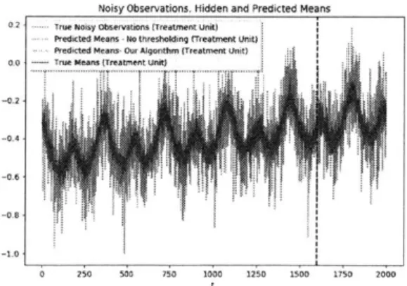
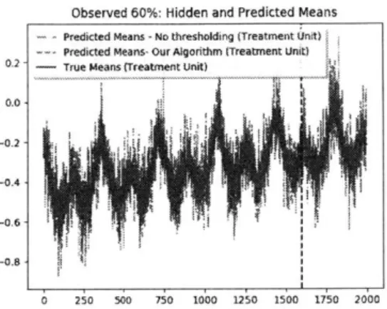
5-9 Treatment unit: noisy observations (gray) and true means (blue) and the estimates from our algorithm (red) and one where no singular value thresholding is performed (green). The plots show all entries normalized to lie in range [-1, 1]. Notice that the estimates in red generated by our model are much better at estimating the true underlying mean (blue) when compared to an algorithm which performs no singular value

thresholding. . . . . 42

5-10 Same dataset as shown in Figure 5-9 but with 40% data missing at

random. Treatment unit: not showing the noisy observations for clarity; plotting true means (blue) and the estimates from our algorithm (red) and one where no singular value thresholding is performed (green). The plots show all entries normalized to lie in range [-1, 1]. . . . . 43

6-1 Trends in per-capita GDP between Basque Country vs. synthetic Basque Country. . . . . 53

6-2 Trends in per-capita GDP between Basque Country vs. synthetic Basque Country. . . . . 54

7-2 Trends in per-capita GDP between Basque Country vs. synthetic Basque Country. . . . . 61 7-3 Trends in per-capita cigarette sales between California vs. synthetic

List of Tables

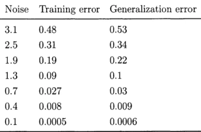
5.1 Training vs. generalization error . . . . 44

Chapter 1

Introduction

Consider a typical comparative case-study where a legislative body is interested in measuring the impact of a policy (e.g. gun control through crime-rate) on a "treated" unit (e.g. California). Unlike the setting of "randomized control" a la A/B testing, the population of such a comparative case-study is limited to a single unit, forcing one to choose an unaffected unit as a "control" (e.g. New York). Historically, such selection was left to the discretion of domain experts. In their seminal work, Abadie and Gardeazabal [4] introduced the concept of "synthetic control", where the control unit is a convex combination of unaffected units (e.g. 80% New York, 20% Massachusetts). Theirs and various subsequent works proposed to learn the synthetic control by applying domain expertise to carefully select the candidate "donor pool" of control units, and utilizing supplementary covariates (e.g. employment rates) to learn the convex relationship.

As the main result of this work, we propose a "robust" approach to finding the synthetic control, wherein we first "noise" the observation data and then use the de-noised data to learn a linear relationship. The de-noising step is a distinguishing feature from prior approaches as it renders the selection of the synthetic control robust in two senses: one, it does not require the assistance of covariates or domain "experts"; and two, it can handle missing and/or noisy observations, an aspect that has not been previously addressed. Under a more general framework that encompasses existing models, we provide finite sample analysis and, subsequently, establish asymptotic consistency, which has been absent from literature. We also analyze the synthetic control method from a Bayesian perspective, which allows our algorithm to go beyond point estimates in expressing our uncertainties through posterior probability distributions. Using real-world datasets, we showcase the robustness of our algorithm by reproducing existing case studies without the benefits of additional covariates or domain knowledge, and in

the presence of missing information. Finally, we generate model-driven synthetic data to validate the efficacy of our algorithm.

1.1

Motivation

On November 8, 2016 in the aftermath of several high profile mass-shootings, voters in California passed Proposition 63 in to law [8]. Prop. 63 "outlaw[ed] the possession of ammunition magazines that [held] more than 10 rounds, requir[ed] background checks for people buying bullets," and was proclaimed as an initiative for "historic progress to reduce gun violence" [25]. Imagine that we wanted to study the impact of Prop.

63 on the rates of violent crime in California. Randomized control trials, such as

A/B testings, have been successful in establishing effects of interventions by randomly exposing segments of the population to various types of interventions. Unfortunately, a randomized control trial is not applicable in this scenario since only one California exists. Instead, a statistical comparative study could be conducted where the rates of violent crime in California are compared to a "control" state after November 2016, which we refer to as the post-intervention period. To reach a statistically valid

conclusion, however, the control state must be demonstrably similar to California sans the passage of a Prop. 63 style legislation. In general, there may not exist a natural control state for California, and subject-matter experts tend to disagree on the most appropriate state for comparison.

As a suggested remedy to overcome the limitations of a classical comparative study outlined above, Abadie et al. proposed a powerful, data-driven approach to construct a "synthetic" control unit absent of intervention [1, 4, 2]. In the example above, the synthetic control (synthetic control) method would construct a "synthetic" state of California such that the rates of violent crime of that hypothetical state would best match the rates in California before the passage of Prop. 63. This synthetic California can then serve as a data-driven counterfactual for the period after the passage of Prop.

63. Abadie et al. propose to construct such a synthetic California by choosing a convex

combination of other states (donors) in the United States. For instance, synthetic California might be 80% like New York and 20% like Massachusetts. This approach is nearly entirely data-driven and appeals to intuition. For optimal results, however, the method still relies on subjective covariate information, such as employment rates, and the presence of domain "experts" to help identify a useful subset of donors. The approach may also perform poorly in the presence of non-negligible levels of noise and missing data.

1.2

Overview of Main Contributions

In this work, we revisit the study of synthetic control from a robust perspective in order to address the limitations described above. As the main result, we propose a simple, two-step robust synthetic control algorithm, wherein the first step de-noises the data and the second step learns a linear relationship between the treated unit and the donor pool under the de-noised setting. The algorithm is robust in two senses: first, it is fully data-driven in that it does not require domain knowledge or the use of supplementary covariate information; and second, it provides the means to overcome the challenges presented by missing and/or noisy observations. As another important contribution, we establish analytic guarantees (finite sample analysis and asymptotic consistency) - that are missing from the literature - for a broader class of models.

1.2.1

Robust algorithm

A distinguishing feature of our work is that of de-noising the observation data via

singular value thresholding. Although this spectral procedure is commonplace in the matrix completion arena, it is novel in the realm of synthetic control. Despite its simplicity, however, thresholding brings a myriad of benefits and resolves points of concern that have not been previously addressed. For instance, while classical methods have not even tackled the obstacle of missing data, our approach is well equipped to impute missing values as a consequence of the thresholding procedure. Additionally, thresholding can help prevent the model from overfitting to the idiosyncrasies of the data, providing a knob for practitioners to tune the "bias-variance" trade-off of their model and, thus, reduce their mean square error (MSE). From empirical studies, we hypothesize that thresholding may possibly render auxiliary covariate information (vital to existing methods) as a luxury as opposed to a necessity.

In the spirit of combatting overfitting, we further extend our algorithm to include regularization techniques such as ridge regression and LASSO. We also move beyond point estimates in establishing a Bayesian framework, which allows one to quantitatively compute the uncertainty of their results through posterior probabilities.

1.2.2

Theoretical performance

To the best of our knowledge, our exposition is the first to analyze both the efficacy of the synthetic control estimator with respect to the MSE and the effect of missing data on the algorithm's performance. Previously, the main theoretical result from the

synthetic control literature pertained to asymptotic unbiasedness for a linear factor model; however, the proof of the result assumed that the latent parameters, which live in the simplex, have been perfectly discovered. We provide finite sample analysis that not only highlights the value of thresholding in balancing the "bias-variance" trade-off, but also proves that the efficacy of our algorithm degrades gracefully with an increasing number of randomly missing data. Further, we show that a computationally beneficial pre-processing step allows us to establish the asymptotic consistency of our least-squares estimator in generality. Using results from the statistical learning theory literature, we provide post-intervention/generalization error bounds under the regularized (ridge regression) setting.

Additionally, we prove a simple linear algebraic fact that justifies the basic premise of synthetic control, which has not been formally established in literature, i.e. the linear relationship between the treatment and donor units exists in the pre- and post-intervention periods. Finally, we introduce a latent variable model, which subsumes many of the models previously used in literature (e.g. econometric factor models). Despite this generality, a unifying theme that connects these models is that they all induce (approximately) low rank matrices, which is well suited for our method.

1.2.3

Experimental results

We conduct two sets of experiments: (a) on existing case studies from real world datasets referenced in [1, 2, 41, and (b) on synthetically generated data. Remarkably, while [1, 2, 41 use numerous covariates and employ expert knowledge in selecting their donor pool, our algorithm achieves similar results without any such assistance; addi-tionally, our algorithm detects subtle effects of the intervention that were overlooked

by the original synthetic control approach. Since it is impossible to simultaneously observe the evolution of a treated unit and its counterfactual, we employ synthetic data to validate the efficacy of our method. Using the MSE as our evaluation metric, we demonstrate that our algorithm is robust to varying levels of noise and missing data, reinforcing the importance of de-noising.

1.3

Related Literature

The study of synthetic control (synthetic control) has received widespread attention ever since its conception by Abadie and Gardeazabal in their pioneering work [4, 1]. It has been employed in numerous case studies, ranging from criminology [261 to

health policy [23] to online advertisement to retail; other notable studies include

[3, 9, 5, 7]. In their paper on the state of applied econometrics for causality and

policy evaluation, Athey and Imbens assert that synthetic control is "one of the most important development[s] in program evaluation in the past decade" and "arguably the most important innovation in the evaluation literature in the last fifteen years"

[6]. In a somewhat different direction, Hsiao et al. introduce the panel data method [20, 21], which seems to have a close bearing with some of the approaches of this work. In particular, [20, 21] only uses data for the outcome variable and solves an ordinary least squares problem in learning synthetic control. However, [20, 21] restrict the subset of possible controls to units that are within the geographical or economic proximity of the treated unit. Therefore, there is still some degree of subjectivity in the choice of the donor pool. In addition, [20, 21] do not include a "de-noising" step, which is a key feature of our approach. For an empirical comparison between the synthetic control and panel data methods, see [19]. It should be noted that [19] also adapts the panel data method to automate the donor selection process. [15] relaxes the convexity aspect of synthetic control, and allows for an additive difference between the treated unit and donor pool, similar to the difference-in-differences (DID) method. In an effort to infer the causal impact of market interventions, [12] introduce yet another evaluation methodology based on a diffusion-regression state-space model that is fully Bayesian; similar to [1, 4, 20, 21], their model also generalizes the DID procedure. Due to the subjectivity in the choice of covariates and predictor variables,

[181 provide recommendations for specification-searching opportunities in synthetic

control applications.

Matrix completion and factorization approaches are well-studied problems with broad applications (e.g. compressed sensing, recommendation systems, etc.). As shown profusely in the literature, spectral methods, such as singular value decomposition and thresholding, provide a procedure to estimate the entries of a matrix from partial and/or noisy observations [13]. With our eyes set on achieving "robustness", spectral methods become particularly appealing since they de-noise random effects and impute missing information within the data matrix [22]. For a detailed discussion on the topic, see [14]; for algorithmic implementations, see [24] and references there in. We note that our goal differs from traditional matrix completion applications in that we are using spectral methods to estimate a low-rank matrix, allowing us to determine a linear relationship between the rows of the mean matrix. This relationship is then projected into the future to determine the counterfactual evolution of a row in the matrix (treated unit), which is traditionally not the goal in matrix completion applications.

Despite its popularity, there has been less theoretical work in establishing the consistency of the synthetic control method or its variants. [1] shows that the synthetic control method can produce an asymptotically unbiased estimator, but under restrictive settings; their analysis relies on the assumption that there not only exists a perfect "convex" match between the pre-treatment noisy outcome and covariate variables for the treated unit and donor pool, but that the algorithm has also discovered the true "convex" weights. In contrast, our analysis does not assume that the estimator has discovered the true set of linear weights and is truly assumption free. [17 also relaxes the strong assumption in [11, and derives conditions under which the synthetic control estimator is asymptotically unbiased. To our knowledge, however, no prior work has provided finite-sample analysis, analyzed the performance of these estimators with respect to the mean-squared error (MSE), established asymptotic consistency, or addressed the possibility of missing data, a common handicap in practice.

1.4

Organization of the Thesis

The rest of this work is outlined as follows: Section 2 describes our notation, setting, and proposed data model. We present the two-step algorithm in Section 3 with the corresponding theoretical and experimental results in Section 4 and Section 5, respectively. We then extend our framework to incorporate regularization methods in Section 6, and finish with a Bayesian treatment of synthetic control in Section 7. All proofs and derivations are unveiled in the appendices.

Chapter 2

Preliminaries

2.1

Setup

In this section, we define the necessary notation and describe the setting.

2.1.1

Notation

We will denote R as the field of real numbers. For any positive integer N, let

[N] {1, ... , N}. For any vector v E R', we denote its Euclidean (f2) norm by

11 V12, and define IIvI1= E, 1V. We define its infinity norm as IIv 11, = maxi IviI. In

general, the f, norm for a vector v is defined as ||vjj =

(z

il) .

an m x n real-valued matrix A = [Aij], _{its spectral/operator norm, denoted by J|Al}

2

,

is defined as

JAIL2

values of A. The Moore-Penrose pseudoinverse At of A is defined as

k At = (1/a)yix[, (2.1) where k A T Xi y, (2.2)

with xi and y, being the left and right singular vectors of A, respectively.

Let b be a random vector that is an estimate of v. Then one choice for the measure of error in estimation is the average mean-squared error, denoted as MSE(b), and

defined as

MSE() = -IIV - I. (2.3)

n 2

We will denote the root mean-squared error, RMSE(), as the square root of the MSE. Since we will frequently use the f2 and spectral norms, we will adopt the shorthand notation of |HJI - || for both cases by often dropping the subscript. Finally, to avoid any confusions between scalars/vectors and matrices, we will represent all matrices in

bold, e.g. A.

2.1.2

Model

The data at hand is a collection of time series with respect to an aggregated metric of interest (e.g. violent crime rates) comprised of both the treated unit (X1) and the

donor pool (X) outcomes. Suppose we observe N > 2 units across T > 2 time periods. We denote To as the number of pre-intervention periods with 1 < To < T, rendering T - To as the length of the post-intervention stage. Without loss of generality, let the

first unit represent the treatment unit - exposed to the intervention of interest at time

t = To + 1. The remaining donor units, 2 < i < N, are unaffected by the intervention

for the entire time period [T] = {1, ... , T}.

In order to distinguish the pre- and post-intervention periods, we use the following notation for all (donor) matrices: A = [A~, A+], where A- = [AijI2 iN,jE[To] and

A+ = [Aij]2iN,To<j T denote the pre- and post-intervention submatrices, respectively; vectors will be defined in the same manner, i.e. Ai = [A-, At], where A- = [Ait]te[ToI

and A = [Ait]To<t T denote the pre- and post-intervention subvectors, respectively, for the ith donor. Moreover, we will denote all vectors related to the treatment unit with the subscript "1", e.g. A1 = [A-, Af].

Let Xit denote the measured value of metric for unit i at time t. We posit Xit= Mit + Eit, (2.4) where Mit is the deterministic mean while the random variables Eit represent zero-mean noise that are independent across i, t. Following the philosophy of latent variable models, we further posit that for all 2 < i < N, t E [T]

where 6 E Rd, and pt E Rd2 are latent feature vectors capturing unit and time specific

information, respectively, for some dj, d2 >

1;

f

:

-

R

captures the model relationship. We note that this formulation subsumes popular econometric factor models, such as the one presented in [1], as a special case with

(small) constants di = d2 and

f

The treatment unit obeys the same model relationship during the pre-intervention period. That is, for t < To

Xi = M + Ci, (2.6)

where Mit f(01, pt) for some latent parameter 01 E R . If unit one was never

exposed to the intervention, then the same relationship as (2.6) would continue to hold during the post-intervention period as well. In essence, we are assuming that the outcome random variables for all unaffected units follow the model relationship defined

by (2.6) and (2.4). Therefore, the "synthetic control" would ideally help estimate

the underlying counterfactual means Mi= f(01, pt) for To < t < T by using an appropriate combination of the post-intervention observations from the donor pool since the donor units are immune to the treatment.

To render this feasible, we make the key operating assumption (as done in literature) that the mean vector of the treatment unit over the pre-intervention period, i.e. the

vector M7 = [Mlt]tTO, lies within the span of the mean vectors within the donor

pool over the pre-intervention period, i.e. the span of the donor mean vectors

Mi- = [Mit]2 iN,tTo '. More precisely, we assume there exists a set of weights

13 E RN-1 such that for all t < To,

N

M

3

i3Mit.

(2.7)

i=2

This is a reasonable and intuitive assumption, utilized in literature, hypothesizing that the treatment unit can be modeled as some combination of the donor pool. In fact, the set of weights # are the very definition of a synthetic control.

In contrast with the classical synthetic control work, we allow our model to be robust to incomplete observations. To model randomly missing data, the algorithm observes each data point Xit in the donor pool with probability p E (0, 1], independently

'We note that this is a minor departure from the literature on synthetic control starting in [41

-in literature, the pre--intervention noisy observation (rather than the mean) vector X1, is assumed to

be a convex (rather than linear) combination of the noisy donor observations. We believe our setup

Chapter 3

Algorithm

We will begin by providing intuition behind our proposed algorithm: (1) we begin

by de-noising our data via singular value thresholding, a distinguishing feature from

prior approaches. Since the singular values of our observation matrix, X, encode both signal and noise, we attempt to find a proper low rank approximation of X that only incorporates the singular values associated with useful information; simultane-ously, this procedure will naturally impute any missing observations. (2) using the pre-intervention portion of the de-noised matrix, we learn the linear relationship be-tween the treatment unit and the donor pool prior to estimating the post-intervention counterfactual outcomes. Since our objective is to produce accurate predictions, it is not obvious why the synthetic treatment unit should be a convex combination of its donor pool as assumed in [1, 4, 3]. In fact, one can reasonably expect that the treatment unit and some of the donor units may exhibit negative correlations with one another. In light of this intuition, we learn the optimal set of weights via linear regression, allowing for both positive and negative elements.

Note: To simplify the exposition, we assume the entries of X are bounded by one in

absolute value, i.e.

IXiti

3.1

Parametrized Algorithm

The algorithm utilizes the thresholding hyperparameter p > 0, which serves as a

knob to effectively trade-off between the bias and variance of the estimator. We discuss the procedure for determining the parameter p soon after the description of the parametrized algorithm.

Step 1. De-noising the data

1. Define

Y = [Yi]

if Xij is observed otherwise.

2. Compute the singular value decomposition of Y:

N-1

S

T

Y = seii.

3. Let S {i : si > p} be the set of singular values above the threshold p.

4. Define the estimator of M as

NI =siuivf Ti E s [ PiES

where

P

Step 2. Learning and projecting

1. Let

3

/3

3 = arg min Y1- -( ) 2

vERN-1

2. Define the counterfactual means for the treatment unit as

1'1

(3.4)

(3.5)

3.1.1

Bounded entries transformation

Several of our results, as well as the algorithm we propose, assume that the observation matrix is bounded such that IXit

I

using the following pre-processing transformation: suppose the entries of X belong to an interval [a, b]. Then, one can first pre-process the matrix X by subtracting (a + b)/2 from each entry, and dividing by (b - a)/2 to enforce that the entries lie in

0,

(3.2)

the range [-1, 1]. The reverse transformation, which can be applied at the end of the algorithm description above, returns a matrix with values contained in the original range. Specifically, the reverse transformation equates to multiplying the end result

by (b - a)/2 and adding by (a + b)/2.

3.1.2

Choosing the hyperparameter, it

Here, we discuss several approaches to choosing the hyperparameter p for the singular values. If it is known a priori that the underlying model is low rank with rank at most

k, then it may make sense to choose p such that ISI = k. A data driven approach,

however, could be implemented based on cross-validation. Precisely, reserve a portion of the pre-intervention period for validation, and use the rest of the pre-intervention data to produce an estimate 3 for each of the finitely many choices of p (S...,

SN-1)-Using each estimate /, produce its corresponding treatment unit mean vector over the validation period. Then, select the 1t that achieves the minimum MSE with respect to the observed data. Finally, [14] provides a universal approach to picking a threshold. As discussed in Section 5, we utilize the data driven approach for producing our results.

3.1.3

Scalability

In terms of scalability, the most computationally demanding procedure is that of evaluating the singular value decomposition (SVD) of the observation matrix. Given the ubiquity of SVD methods in the realm of machine learning, there are well-known techniques that enable computational and storage scaling for SVD algorithms. For instance, both Spark (through alternative least squares) and Tensor-Flow come with built-in SVD implementations. As a result, by utilizing the appropriate computational infrastructure, our de-noising procedure, and algorithm in generality, can scale quite well.

3.1.4

Remarks on low-rank hypothesis

The factor models that are commonly used in the Econometrics literature, cf. [1, 2, 4], often lead to a low-rank structure for the underlying mean matrix M. When

f

f

well approximated by a low-rank matrix, cf. see [14] for a very simple proof. As the reader will notice, while we establish results for low-rank matrix, the results of this work are robust to low-rank approximations whereby the approximation error can be viewed as "noise". Lastly, as shown in [27], many latent variable models can be well approximated (up to arbitrary accuracy E) by low-rank matrices. Specifically, [27] shows that the corresponding low-rank approximation matrices associated with "nice" functions (e.g. linear functions, polynomials, kernels, etc.) are of log-rank.

Chapter 4

Summary of Main Results

In this section, we derive the finite sample and asymptotic properties of the esti-mator, M1. We begin by defining necessary notations and recalling a few operating

assumptions prior to presenting the results, with the corresponding proofs relegated to the Appendix. To that end, we re-write (2.4) in matrix form as X = M + E, where E = [Eit]2<i<N,tE[T} denotes the noise matrix. We shall assume that the noise

parameters Eit are independent zero-mean random variables with bounded second moments. Specifically, for all 2 < i < N, t

E

E[Ect] = 0, and Var(Eit) < 02. (4.1)

We shall also assume that the treatment unit noise in (2.6) obeys (4.1). Further, we assume the relationship in (2.7) holds.

As previously discussed, we wish to evaluate the accuracy of our estimated means for the treatment unit with respect to the MSE, i.e. the deviation between M{_ and M7 measured in f2-norm. Additionally, we aim to establish the validity of our

pre-intervention linear model assumption (cf. (2.7)) and investigate how the linear relationship translates over to the post-intervention regime, i.e. if M- = (M-)TI3 for some 3, does M1+ (approximately) equal to (M+)Tf3 and if so, under what conditions? We now present our results for the above two aspects.

4.1

Pre-intervention analysis

The performance metric of interest is the average mean squared error in estimating

ME using Mi-. Precisely, we define

MSE(Mi-) = E[ (Mu - Mi)2. (4.2)

TO t=1

We say that M(- is a consistent estimator if (4.2) approaches 0 as To -+ oo. In what

follows, we first state the finite sample bound on (4.2) for the most generic setup

(Theorem 4.1.1). As a main Corollary of the result, we specialize the bound in the case where M is low-rank. (Corollary 4.1.1). Finally, we discuss a minor variation of the algorithm where the data is pre-processed, and specialize the above result to establish the consistency of our estimator (Theorem 4.1.2).

4.1.1

General result

We provide a finite sample error bound for the most generic setting.

Theorem 4.1.1. The pre-intervention error of the algorithm can be bounded as

MSE( -) < 2_{To E(A* + Y -pM1} +Yp _{+ 1(p -p)M-11) I/#2 + (4.3)} + C2(N - 1)I10112 e-p(N-1)T (4.4)

Here, A, . . ., AN- 1 are the singular values of pM in decreasing order and repeated by

multiplicities, with A* = maxios A ; C1, C2 and c are universal positive constants.

Let us interpret the result by parsing the terms in the error bound. The last term decays exponentially with (N - 1)T, as long as the fraction of observed entries is

such that, on average, we see a super-constant number of entries, i.e. p(N - 1)T

>

More interestingly, the first two terms highlight the "bias-variance tradeoff" of the algorithm with respect to the singular value threshold p. Precisely, the size of the set

S increases with a decreasing value of the hyperparameter p, causing the second error

term to increase. Simultaneously, however, this leads to a decrease in A*. Note that A* denotes the aspect of the "signal" within the matrix M that is not captured due to the thresholding through S. On the other hand, the second term,

ISl.2 /To,

model may fail to capture pertinent information encoded in M; if we use a small threshold, then the algorithm may overfit the spurious patterns in the data. Thus, the hyperparameter p provides a way to trade-off "bias" (first term) and "variance" (second term).

4.1.2

Goldilocks Principle

With an appropriate choice for the hyperparameter p (and hence S), we state the following result for the specialized setting whereby the signal matrix M is low rank.

Corollary 4.1.1. Let rank(M) = k for some 1 < k < N - 1. Let the choice of P be such that |SI = k. Suppose cr2p + p(l - p) > T-1 + for some ( > 0. Let T < aTo for

some constant a > 1. Then

Ci

1,31I

lim MSE(Mj-) < (a + (1 - p)). (4.5)

To--oo _p

By adroitly capturing the signal, the resulting error bound simply depends on

the variance of the noise terms, ou2, and the error introduced due to missing data. Ideally, one would hope to overcome the error term when To is sufficiently large. This motivates the following setup.

4.1.3

Asymptotic Consistency

We present a straightforward pre-processing step that leads to the asymptotic consis-tency of our algorithm. The pre-processing step simply involves replacing the columns of X by the averages of its columns. This admits the same setup as before, but with the variance for each noise term reduced. An implicit side benefit of this approach is that required SVD step in the algorithm is now applied to smaller size matrix.

Partition the To columns of the pre-intervention data matrix X- into T = _/ToJ

blocks, each of size r except potentially the last block. Let B, =

{(j

j

practice, however, the remaining columns can be placed into the last block. Next, we replace the T columns within each partition by their average, and thus create a new

matrix, X~, with T columns and N - 1 rows. Precisely, X [Xij]2 i<N,jr with

Xij

S

T

Let

M-

li = : Mit. _(4.7)

7tEBj

We apply the algorithm to X- to produce the estimate

M-

M-,

to estimate 3. This 3 can be used to produce the post-intervention synthetic control

means Mj = [Mit] To<t in a similar manner as before 1: for To < t < T,

N

1t

= E

ixit.

(4.8)

i=2

For the pre-intervention period, we produce the estimator M-= [M13]1j<r :: for

<

j

<

T,

N

i / = iMij. (4.9)

i=2

Our measure of estimation error is defined as

MSE(M;) =-E (Mi3 - Mi9)]. (4.10)

1<j<Tr

We state the following result.

Theorem 4.1.2. Let rank(M-) = k for some 1 < k < N - 1. Let the choice of p be

such that |SI= k. Then

lim MSE(M7) = 0.

To-*oo

We note that the method of

14,

the data. One common pre-processing proposal is to also aggregate the columns, but the aggregation parameters are chosen by solving an optimization problem to minimize the resulting prediction error of the observations. In that sense, the above averaging of column is a simple, data agnostic approach to achieve a similar effect, and potentially more effectively.

'In practice, one can first de-noise X+ via step one of Section 3, and use the entries of MI+ in

4.2

Post-intervention analysis (static rank)

The key assumption of our analysis is that the treatment unit signal can be written as a linear combination of donor pool signals. Specifically, we assume that this relationship holds in the pre-intervention regime, i.e. Mj- = (M-)T/3 for some 3 E RN-1 as stated

in (2.7). The question still remains, however, does the same relationship hold for the post-intervention regime and if so, under what conditions does it hold? We state a simple linear algebraic fact to this effect, justifying the entire approach of synthetic control. It is worth noting that this important aspect has been amiss in the literature, potentially implicitly believed or assumed starting in the work by [4].

Theorem 4.2.1. Let (2.7) hold for some /. Let rank(M-) = rank(M). Then

= (M+)TI3.

If we assume that the linear relationship prevails in the post-intervention period,

then we arrive at the following error bound.

Theorem 4.2.2. Assuming rank(M-) = rank(M), the post-intervention error is

bounded above by RMSE(M+) < E A* +1Y - pM 1 + ( p)M+ + E - 3 pP T-To VT -TO C2VTo(N - 1) ep(N-1)T + e ft

Here, A,..., AN-, are the singular values of pM in decreasing order and repeated by multiplicities, with A* = maxios Ai; C1, C2, and c are universal positive constants.

Let us interpret the post-intervention error bound by decomposing the RMSE into two error terms (we will ignore the third expression since it decreases exponentially fast with the size of the training set): the first error term derives from the de-noising/estimation error from Step one of our robust algorithm, and the second term captures the learning algorithm's error (in this case, linear regression) from Step two. Similar to the pre-intervention error, there is a trade-off between "bias" and "variance", which is dictated by the choice of the threshold value M. To see this, we analyze

the key information ratio A*/p within the first term. As p increases, our de-noising process uses less singular values (smaller set S), rendering A* - the signal not captured in the thresholding process - to also increase. On the flip side, if we use a small threshold, then we are utilizing most of the data matrix's singular values, yielding A*

to also decrease. In either case, there is a tension that exists due to the thresholding procedure since A* and p are positively correlated.

The second error term, which is controlled by the expression

i

of the learning algorithm used to estimate /. As we will shortly see, using regularization

can decrease the MSE between

/

/,

Chapter 5

Experimental Results

We begin by exploring two real-world case studies discussed in [1, 2, 4] that demon-strate the ability of the original synthetic control's algorithm to produce a reliable counterfactual reality. We use the same case-studies to showcase the "robustness" property of our proposed algorithm. Specifically, we demonstrate that our algorithm reproduces similar results even in presence of missing data, and without knowledge of the extra covariates utilized by prior works. We find that our approach, surprisingly, also discovers a few subtle effects that seem to have been overlooked in prior studies. For the purposes of this section, we refer to the algorithm presented in Section 3 as robust synthetic control (linear). Additionally, we introduce a variation to our proposed algorithm by restricting

/

As described in [1, 2, 3], the synthetic control method allows a practitioner to evaluate the reliability of his or her case study results by running placebo tests. One such placebo test is to apply the synthetic control method to a donor unit. Since the control units within the donor pool are assumed to be unaffected by the intervention of interest (or at least much less affected in comparison), one would expect that the estimated effects of intervention for the placebo unit should be less drastic and divergent compared to that of the treated unit. Ideally, the counterfactuals for the placebo units would show negligible effects of intervention. Similarly, one can also perform exact inferential techniques that are similar to permutation tests. This can be done by applying the synthetic control method to every control unit within the donor pool and analyzing the gaps for every simulation, and thus providing a distribution of estimated gaps. In that spirit, we present the resulting placebo tests for the Basque

'In the Econometrics literature, an emphasis has been placed on having [ being "convex" as it provides an intuitive interpretation: the treatment unit is proportionately like the donor units.

Country and California Prop. 99 case studies below to assess the significance of our estimates.

5.1

Basque Country

The goal of this case-study is to investigate the effects of terrorism on the economy of Basque Country using the neighboring Spanish regions as the control group. In

1968, the first Basque Country victim of terrorism was claimed; however, it was not

until the mid-1970s did the terrorist activity become more rampant [4]. To study the economic ramifications of terrorism on Basque Country, we only use as data the per-capita GDP (outcome variable) of 17 Spanish regions from 1955-1997. We note that in [41, 13 additional predictor variables for each region were used including demographic information pertaining to one's educational status, and average shares for six industrial sectors.

5.1.1

Results

Figure 5-la shows that our method (both linear and convex) produces a very similar qualitative synthetic control to the original method even though we do not utilize additional predictor variables. Specifically, the synthetic control resembles the observed GDP in the pre-treatment period between 1955-1970. However, due to the large-scale terrorist activity in the mid-70s, there is a noticeable economic divergence between the synthetic and observed trajectories beginning around 1975. This deviation suggests that terrorist activity negatively impacted the economic growth of Basque Country.

One subtle difference between our (linear and convex) synthetic control and that of [4] is between 1970-75: our approach suggests that there was a small, but noticeable economic impact starting just prior to 1970, potentially due to first terrorist attack in

1968. Notice, however, that the original synthetic control of [4j diverges only after

1975.

To study the robustness of our approach with respect to missing entries, we discard each data point uniformly at random with probability 1 - p. The resulting control for

different values of p is presented in Figure 5-1b suggesting the robustness of our (linear) algorithm. Finally, we produce Figure 5-1c by applying our algorithm without the de-noising step. As evident from the Figure, the resulting predictions suffer drastically, reinforcing the value of de-noising. Intuitively, using an appropriate threshold P equates to selecting the correct model complexity, which helps safeguard the algorithm

from potentially overfitting to the training data.

12 Basque country study Missing at random: Basque Country Study 12 Basque country study

10

igens nw Basque C

Country.ryP ₉

.2 Placeb symtestsWpfwf)Y .

t n snt t tha oysimiartBasque CoAnyun

wert senve n]e.) ftrorism bPs n bt t Vss c ?955 19601965 1970 197S 1950 19115 1990 95S990 16 97 175-90 13 90 19 0D 1i 90 19S 17 95 28 98 90 19

evolutions

~~~~O

year yewr Year

(a) Comparison of methods. (b) Missing data. (c) Impact of de-noising.

Figure 5-1: Trends in per-capita GDP between Basque Country vs. synthetic Basque

Country.

5.1.2

Placebo tests

We begin by applying our robust algorithm to the Spanish region of Cataluna, a control unit that is not only similar to Basque Country, but also exposed to a much lower level of terrorism [2]. Observing both the synthetic and observed economic evolutions of Cataluna in Figure 5-2a, we see that there is no identifiable treatment effect, especially compared to the divergence between the synthetic and observed

Basque trajectories. We provide the results for the regions of Aragon and Castilla Y

Leon in Figures 5-2b and 5-2c.

12 Placebo study: Cataluna Placebo study. Aragon Placebo study: Castilla Y Leon

~11

- 3 -2- - aCataY teon

-- t etsyn A-syntheoc Csuta

io 160 1965 1970 1975 19-0 190 0990 1995 s 196 19s 1970 1971 1980 1909 1990 193s 1955 19655 970 1975 1980 1905 1990 1995

year year year

(a) Cataluna. (b) Aragon. (c) Castilla Y Leon.

Figure 5-2: Trends in per-capita GDP for placebo regions.

Additionally, we performed the exact inferential test on all control regions and plotted the resulting per-capita GDP gaps in Figures 5-3a and 5-3b, whereby Figure

5-3b excluded two control regions; the purpose behind this action will be made clear in

the following paragraph. The resulting figures suggest that there is a low probability of obtaining a large economic divergence similar to that of Basque Country, when we reassign the intervention to the donor regions.

Since there is no ground truth, we continue to use the seminal results of [2] as a baseline. We begin by noting that [2] removed the plots of all five regions that had a poor pre-treatment period fit (regions with a mean-squared error, with respect to some pre-intervention validation period, that is five times greater than that for Basque Country); we display their resulting figure for the 12 remaining regions in Figure

5-4a as a visual reference. As a result, we removed the two regions - Balearic Islands

and Madrid - that were mentioned in [2]. Thus, Figure 5-3a represents the result

of our inferential test on all control regions while 5-3b excludes the Balearic Islands and Madrid. Even though [2] used 13 additional covariates and excluded more "bad" regions from their permutation placebo test, we observe that our results are nearly identical. This reinforces the robustness of our algorithm, highlighting the profound impact of de-noising.

Placebo Study. Basque Country Placebo Study: Basque Country

05 / 05

196. 5

...

.

...

>

year year

(a) Includes all control regions. (b) Excludes 2 regions.

Figure 5-3: Per-capita GDP gaps for Basque Country and control regions.

WO

92

tiMa

(a) Excludes 5 regions.

5.2

California Anti-tobacco Legislation

We study the impact of California's anti-tobacco legislation, Proposition 99, on the per-capita cigarette consumption of California. In 1988, California introduced the first modern-time large-scale anti-tobacco legislation in the United States [1]. To analyze the effect of California's anti-tobacco legislation, we use the annual per-capita cigarette consumption at the state-level for all 50 states in the United States, as well as the District of Columbia, from 1970-2015. Similar to the previous case study, [41 uses 6 additional observable covariates per state, e.g. retail price, beer consumption per capita, and percentage of individuals between ages of 15-24, to predict their synthetic California. Furthermore, [4] discarded 12 states from the donor pool since some of these states also adopted anti-tobacco legislation programs or raised their state cigarette taxes, and discarded data after the year 2000 since many of the control units had implemented anti-tobacco measures by this point in time.

5.2.1

Results

As shown in Figure 5-5a, in the pre-intervention period of 1970-88, our control (linear and convex) matches the observed trajectory. Post 1988, however, there is a significant divergence suggesting that the passage of Prop. 99 helped reduce cigarette consumption. Similar to the Basque case-study, our estimated effect is qualitatively similar to that of [4]. As seen in Figure 5-5b, our (linear) algorithm is again robust to randomly missing data.

Tobacco case study ,Missing at random: Califomia Tobacco Study

p12,112

.100 0

r 5: Tg b California

5.2. PlcbPet

W pb tuso sycthoraOMMd .0e ab

F 20 5oa t syndoc Ctar e icsdonthrl x s f

-Oogoo syr~nec cafrfo

197D 1975 1MO 1905 1990 1Was 2000 1970 1975 1950 1995 1990 1995 2000 2005 2000 2025

(a) Comparison of methods. (b) Missing data.

Figure 5-5: Rends in per-capita cigarette sales between California vs. synthetic California.

5.2.2

Placebo tests

We now proceed to apply the same placebo tests to the California Prop 99 dataset. Figures 5-6a, 5-6b, and 5-6c are three examples of the applied placebo tests on the