Multiscale simulation of heat transfer in a rarefied gas

Multiscale simulation of heat transfer in a rarefied gas

Stephanie Y. Dochertya,∗_{, Matthew K. Borg}a_{, Duncan A. Lockerby}b_{, Jason M. Reese}c

a_{Department of Mechanical & Aerospace Engineering, University of Strathclyde, Glasgow G1 1XJ, UK} b_{School of Engineering, University of Warwick, Coventry CV4 7AL, UK}

c_{School of Engineering, University of Edinburgh, Edinburgh EH9 3JL, UK}

Abstract

We present a new hybrid method for dilute gas flows that couples a continuum-fluid description to the direct simulation Monte Carlo (DSMC) technique. Instead of using a domain-decomposition framework, we adopt a heterogeneous approach with micro reso-lution that can capture non-equilibrium or non-continuum fluid behaviour both close to bounding walls and in the bulk. A continuum-fluid model is applied across the entire domain, while DSMC is applied in spatially-distributed micro regions. Using a field-wise coupling approach, each micro element provides a local correction to a continuum sub-region, the dimensions of which are identical to the micro element itself. Interpolating this local correction between the micro elements then produces a correction that can be applied over the entire continuum domain. Key advantages of this method include its suitability for flow problems with varying degrees of scale separation, and that the location of the micro elements is not restricted to the nodes of the computational mesh. Also, the size of the micro elements adapts dynamically with the local molecular mean free path. We demonstrate the method on heat transfer problems in dilute gas flows, where the coupling is performed through the computed heat fluxes. Our test case is micro Fourier flow over a range of rarefaction and temperature conditions: this case is simple enough to enable validation against a pure DSMC simulation, and our results show that the hybrid method can deal with both missing boundary and constitutive information.

Keywords: heterogeneous multiscale simulation, hybrid methods, DSMC, heat flux coupling, rarefied gas dynamics

1. Introduction

While the conventional hydrodynamic equations are generally excellent for modelling the majority of fluid flow problems, the presence of localised regions of non-continuum or non-equilibrium flow can result in some degree of inaccuracy. Such regions appear when the flow is far from local thermodynamic equilibrium, for example, when there are large gradients in fluid properties, or when surface effects become dominant. Although molecular simulation tools can provide an accurate modelling alternative in these cases,

∗_{Corresponding author. Tel.: +44 7860 366 574}

Email address: [email protected](Stephanie Y. Docherty)

they are usually much too computationally expensive for resolving engineering spatial and temporal scales. Multiscale methodologies that exploit ‘scale separation’ have therefore been developed over the past decade. Scale separation occurs when the variation of hydrodynamic properties across small regions of space or periods of time is only very loosely coupled with the flow behaviour on a much larger spatial or temporal scale.

Often referred to as ‘hybrids’, these multiscale methods combine continuum and molecular descriptions of the flow. A traditional continuum description is employed in macro flow regions, and a molecular treatment is applied in small-scale micro or nano regions. Essentially, the aim is to combine the best of both solvers: the computational efficiency associated with continuum methods, and the detail and accuracy of molecular techniques.

In the literature, two different hybrid frameworks have emerged for fluid flows: a) the domain-decomposition technique, and b) the Heterogeneous Multiscale Method (HMM). For liquids, molecular dynamics (MD) is the appropriate molecular simulation tool. This deterministic method is, however, inefficient for dilute gas flows, and the direct simu-lation Monte Carlo (DSMC) method [1] can instead provide a coarse-grained molecular description. Founded on the kinetic theory of dilute gases, DSMC reduces computational expense by adopting a stochastic approximation for the molecular collision process.

Typically, thermodynamic non-equilibrium effects occur in the vicinity of bounding surfaces or other interfaces. Recognising this behaviour, domain-decomposition has be-come the most popular hybrid framework for both liquids [2, 3, 4, 5, 6] and dilute gases [7, 8, 9, 10, 11, 12, 13, 14, 15, 16, 17]. In this method, the simulation domain is partitioned — a molecular solver is applied in the regions closest to the surfaces, while a conven-tional continuum fluid solver is implemented in the remainder. These micro and macro sub-domains are independent but communicate through an overlap region that enables mutual coupling. This coupling is typically established by matching fluxes of fluid mass, momentum, and energy, or by matching state properties. However, despite its popularity, a fundamental disadvantage of this micro-macro decomposition approach is that compu-tational efficiency can be increased above that of a full molecular simulation only when non-continuum flow is confined to ‘near-wall’ regions. In highly non-equilibrium flows, or when the temperature dependence of fluid properties such as dynamic viscosity or thermal conductivity is not knowna priori (for example, in unusual chemically-reacting gas mixtures), the traditional fluid constitutive relations may be inaccurate in the bulk of the domain.

Domain-decomposition techniques are also inappropriate for simulating flow through micro or nanoscale geometries that have a high aspect ratio, e.g. one dimension of the geometry is orders of magnitude larger than another. This class of flow presents a challenge as it requires simultaneous solution of the microscopic processes occurring over the smallest dimension and the macroscopic processes occurring over the largest dimension, and is often too computationally intensive for a full molecular approach. Such flows are generally beyond the reach of domain-decomposition as the majority (or perhaps all) of the flowfield can be considered ‘near-wall’.

The less-common HMM framework overcomes the limitations of domain-decomposition by adopting a micro-resolution approach that can be employed anywhere in the domain — near bounding surfaces, or in the bulk flow. In this case, a continuum model is applied across the entire flow field, and the molecular solver is applied in spatially-distributed micro regions. These micro regions provide the missing data that is required for closure

of the local continuum model, either in the form of unknown boundary conditions, or unknown constitutive information. Existing HMM studies in the literature are mainly for liquid flows, using MD as the molecular solver [18, 19, 20, 21]. Generally, these studies consider flow problems where momentum transport is dominant and the transfer of heat is negligible. Coupling is therefore based on momentum: velocity fields or strain-rates are prescribed in each micro region, and the resultant stress is used to apply a correc-tion back into the hydrodynamic momentum equacorrec-tion [18, 19]. Each HMM micro region supplies information to a computational node on the continuum mesh. Thispoint-wise coupling approach [20] is ideal when there is a large degree of spatial scale separation in the system, providing significant computational savings over a pure molecular simulation. However, in flow problems with smaller, or mixed, degrees of spatial scale separation, the molecular resolution required can result in the micro elements overlapping, making HMM more expensive and less accurate than a pure molecular treatment.

Despite its advantages over domain-decomposition techniques, there has been little development of HMM-type hybrids that use DSMC as the molecular treatment. In 2010, Kessleret al. [22] proposed the Coupled Multiscale Multiphysics Method (CM3₎

that couples both momentum and heat transfer, with DSMC providing corrections to both the hydrodynamic momentum and energy equations. This method was, however, developed to simulate transient flows where a time-accurate solution is sought, and so any computational advantage over a full DSMC simulation is achieved only through decoupling of the time scales; the length scales remain fully coupled, with both the continuum description and DSMC employed over the same region of space. More recently, Patroniset al.[23] adapted the Internal-flow Multiscale Method (IMM) to simulate dilute gas flows with DSMC. Originally developed by Borg et al. [21] for liquid flows, IMM adopts a framework similar to HMM but is tailored to model flows in high-aspect-ratio channels. Although large computational savings are presented, this method is tailored specifically to deal with cases where the length scale in the direction of flow is significantly larger than the length scales transverse to the flow direction.

In this paper we propose a new form of the HMM technique, with DSMC providing the molecular description. We adopt the field wise coupling (HMM-FWC) approach developed by Borget al. [24] for liquid flows: rather than supplying a correction to a node on the continuum mesh, each micro element instead corrects a continuum sub-region, the spatial dimensions of which are identical to those of the micro element itself. This means that, unlike point wise coupling, HMM-FWC is suitable for dealing with flow problems with varying degrees of spatial scale separation. Also, the location of each micro element is not restricted to the nodes of the computational mesh: both the position and size of the micro elements can be optimised for each problem, independently of the continuum mesh.

Our method is designed to cope with inaccuracy in the traditional flow boundary conditions and/or constitutive relations, and is therefore able to deal with problems which are beyond the reach of domain-decomposition. This includes problems where the fluid behaviour is unknown in the bulk, i.e. the traditional constitutive relations fail due to non-equilibrium effects (for example, in the wake of a re-entry vehicle), or the transport properties are unknown (for example, in unusual gas mixtures). The method is also suitable for simulating high aspect ratio geometries. While the IMM is designed to simulate problems where the largest length scale is in the flow direction, our new method has no such restriction and so provides a more general approach. It could therefore be

useful when the largest length scale is transverse to the flow direction; for example, the flow through microscale cracks in valves.

The form of the method we present in this paper is tailored to model heat transfer problems in dilute gas flows. As a starting point we consider problems in which the gas is essentially motionless, with large applied temperature gradients placing the focus on heat transfer. With negligible transport of momentum, our coupling is performed through the heat flux: we impose the local temperature fields on the micro elements and measure the consequent heat flux from the relaxed DSMC particle ensembles. A suitable correction is then applied to the hydrodynamic conservation of energy equation. (Full coupling of mass, momentum, and heat transfer is a subject for future work.)

The level of translational non-equilibrium in a rarefied gas is generally characterized by the Knudsen number Kn, defined as the ratio of the gas molecular mean free path λ to a characteristic system dimension L. Typically, the traditional ‘no-temperature-jump’ boundary condition at a bounding surface (wall) is only valid whenKn <0.001; the flow is then in thermodynamic equilibrium as the frequency of both intermolecular and molecule-wall collisions is very high. As Kn increases above 0.001, this collision frequency decreases, resulting in a temperature discontinuity between the wall and its adjacent gas. For lowKn, the conventional conservation equations can be extended to account for this by employing von Smoluchowski temperature-jump boundary conditions [25]. However, as Kn increases, molecule-wall collisions become more frequent than intermolecular collisions and a thermal Knudsen layer develops. This is essentially a region of non-equilibrium that extends from the wall into the domain, with its thickness determined by the degree of rarefaction. In this layer, the gas behaviour deviates from the conventional linear heat flux/temperature-gradient constitutive relation. Even with the use of temperature-jump boundary conditions, the conventional hydrodynamic equations cannot model this phenomenon. Our hybrid method, however, aims to capture both the temperature-jump and the thermal Knudsen layer at a lower computational cost than a full-domain DSMC treatment.

This paper is organised as follows. In Section 2, we discuss the macro and micro descriptions of the flow. We then present the general three-dimensional form of our mul-tiscale coupling framework and its iterative algorithm. For simplicity, one-dimensional heat transfer is considered when validating the method in Section 3, with results com-pared with pure DSMC simulations at equivalent conditions. In Section 4 we draw our conclusions.

2. Multiscale methodology

2.1. Continuum description

For simplicity in this paper, we restrict our attention here to steady-state problems where the gas remains stationary, i.e. it has no streaming velocity. With negligible transport of mass and momentum, the continuum description is based on the conservation of energy,

∇ ·q= 0, (1)

whereq is the heat flux vector. To close this equation, a suitable constitutive relation is required. For conventional gas flows, the traditional Navier-Stokes-Fourier (NSF)

constitutive relations are accurate and so Fourier’s law can be used, i.e.

q=−κ∇T, (2)

whereκis the thermal conductivity of the gas. The energy equation then reads,

∇ ·(κ∇T) = 0. (3)

Assuming no-temperature-jump boundary conditions, solution of this conventional en-ergy equation will produce a continuum NSF temperature fieldTNSF. This field is taken

as an initial condition for our hybrid method, and provides a starting point from which the coupling framework iterates towards the correct temperature field.

While Eq. (2) is valid for typical flow problems, it fails in certain flow conditions, for instance, in flows of complex fluids or in conditions of thermodynamic non-equilibrium. Inaccuracy in the conventional constitutive model can therefore be quantified by a heat-flux-correction fieldΦ, so that

q=−κ∇T +Φ. (4)

The flux-correction field incorporates not only the departure of the gas state from equi-librium, but also any additional inaccuracy due to the assumed thermal conductivity model. Using this relation to close Eq. (1) results in a ‘flux-corrected’ energy equation,

∇ ·(κ∇T)− ∇ ·Φ= 0. (5)

The general strategy of our heterogeneous hybrid approach is therefore as follows. Across each individual micro element, the heat flux and temperature fields are mea-sured. The flux-correction field across each element is then computed using Eq. (4). By interpolating between all micro elements, the full flux-correction fieldΦacross the entire flowfield is approximated. With this, and the boundary information obtained from micro simulations located at the bounding walls, an appropriate continuum method (e.g. finite difference, finite element, or finite volume) can be used to solve Eq. (5). This produces a flux-corrected continuum temperature field TΦ across the domain. With continuing

iterations, this temperature field should converge towards that which would be obtained from a full molecular simulation of the problem.

2.2. DSMC technique

As we focus on heat transfer in dilute gases, we use DSMC as our molecular model in the micro elements. DSMC has become the dominant method for simulation of dilute gas flows that lie in the continuum-transition regime. The fundamental concept is to track a large number of numerical particles, storing their position, velocity, and internal state as they move through a computational mesh. During a simulation, the particles collide with each other and with bounding surfaces while maintaining conservation of mass, mo-mentum, and energy. A major advantage of the method is that two key approximations significantly reduce computational expense: (a) each simulated particle typically repre-sents a large number of real gas molecules, and (b) molecular motion and intermolecular collisions can be decoupled over small time intervals. Particle movements are computed deterministically, while interparticle collisions are treated statistically within numerical mesh cells.

Using expressions provided by Bird [1], local hydrodynamic properties (including the temperature and the heat flux) can be recovered in DSMC by averaging microscopic data over all of the particles in each cell. However, the inherent statistical scatter asso-ciated with the method means that a large number of independent samples are usually required to capture smooth fields, particularly for low speed flows. Therefore, time av-eraging is typically used for steady state problems, while ensemble avav-eraging is used for transient flow problems. For continuum-molecular hybrids, the smoothing of statistical fluctuations is particularly important as the transfer of noisy data to the continuum fluid description may result in instability. Consequently, each DSMC simulation in this paper is performed in two stages: a transient period enables the simulation to reach steady-state, then a longer averaging period reduces the statistical scatter in the measured hydrodynamic properties.

The open-source C++ toolbox OpenFOAM [26] incorporates a DSMC solver, dsmc-Foam, which has been validated for various benchmark cases, including hypersonic and microchannel flows [27, 28, 29]. This is used to perform all the micro and full-scale DSMC simulations in this paper.

2.3. Coupling framework

In our framework, the continuum description is applied across the entire macro do-main, while DSMC is performed in dispersed micro elements (the arrangement of which depends on the flow problem being investigated). As discussed in the Introduction, we propose a new strategy to achieve two-way coupling between these domains. The un-derlying methodology presented here is general and may be applied to 1D, 2D, or 3D problems.

2.3.1. Macro-to-micro coupling: constraint of the micro elements

It is crucial that the flux-correction information is extracted from DSMC elements in which the gas state is properly representative of the local conditions in the macro domain. There is, however, a fundamental problem in creating such elements: the par-ticle distribution required at the boundaries of the element cannot be extracted directly from the macroscopic continuum flowfield. For this reason, macro-to-micro coupling re-mains a challenge in multiscale hybrids. In our method, we circumvent this problem by not imposing an exact particle distribution at these boundaries; instead, we allow the distribution to be dictated by the macroscopic continuum fields alone.

A natural evolution to the correct particle distribution and macroscopic state at the boundaries of an element is possible by establishing an artificial relaxation region (zone) around the element. It is not essential that the gas state in these relaxation zones accurately represent the conditions in the corresponding macro domain; their sole purpose is to develop the boundary conditions for the core of the element. Sampling of property fields is performed only in the core region, which we refer to as the ‘sampling zone’.

Suitable boundary conditions to the sampling zone are generated by enforcing the continuum variation of macroscopic properties (i.e. in our case, the continuum tempera-ture field) across the surrounding relaxation zone. This is done by implementing particle controllers [30]. A particle distribution does, however, need to be applied at the outer boundaries of the relaxation zone. This imposed distribution introduces error in the local

distribution close to these boundaries, so it is important that the particle state within the sampling zone is sufficiently independent of this introduced error. If the relaxation zone is large enough (i.e. several molecular mean free paths), the form of the imposed distribution1 _{is irrelevant — its effect will decay through the zone as the particle state}

gradually relaxes through interparticle collisions. Complete relaxation needs to occur over the extent of the relaxation zone such that the particle distribution in the sampling zone is dictated solely by the applied continuum state. Once the hybrid method has converged, the artificiality of the outer relaxation zone dissolves seamlessly into the true particle distribution and fluid state in the inner sampling zone.

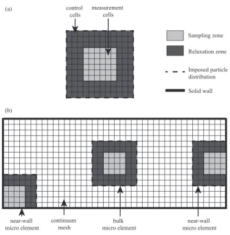
Figure 1(a) shows a typical ‘bulk’ micro element in 2D. Similarly, Fig. 1(b) shows an example computational domain set-up for a 2D problem, including both bulk and ‘near-wall’ micro elements. In summary, the sampling zone in a micro element is surrounded by the relaxation zone over which the local continuum fields are imposed, and a chosen particle distribution is applied at the outer boundaries. However, in order to capture regions of non-equilibrium that often appear at solid bounding surfaces or walls, the sampling zone in a near-wall micro element must be adjacent to the wall itself. The arrangement of the micro elements is clearly crucial to the resulting accuracy of our method, and the appropriate arrangement will vary from problem to problem.

To impose the local continuum temperature field, we divide the relaxation zone in each micro element into a grid of control cells as shown in Fig. 1. Using particle controllers [30], the appropriate temperature is then set in each control cell to create the desired temperature variation. Similarly, the sampling zone of each micro element is divided into a grid of measurement cells. We then extract the averaged hydrodynamic properties from each measurement cell, enabling us to capture the property fields across the entire sampling zone. Boundary information is also obtained from these measurement cells: we extract the temperature of the gas in contact with the wall from the wall-adjacent cell faces.

Essentially, these measurement and control cells form a measurement/control mesh that is completely independent of the computational mesh used by DSMC itself. This has the benefit of enabling us to define the resolution of the macroscopic fields that we both extract and impose, and to control the noise in our measurements, without affecting the accuracy of the DSMC calculations (i.e. the particle collision rate). In Fig. 1, the measurement and control cells are shown to have the same dimensions, but this does not have to be the case. Also, in Fig. 1(b), the measurement and control cells are shown to be collocated with the computational cells of the continuum mesh; although this simplifies the transfer of data between the micro elements and the continuum description, it is only for convenience and is not essential. If these cells are not collocated, we simply interpolate between the meshes.

2.3.2. Micro-to-macro coupling: correcting the continuum description

The ease in converting microscopic particle information into macroscopic fields means that, generally, micro-to-macro coupling is less problematic than macro-to-micro cou-pling. Based on the property fields extracted from the DSMC solver, a suitable correction

1_{We implement local Maxwellian distributions at the outer edges of the relaxation zones for simplicity.}

Chapman-Enskog distributions could also be used; as these include perturbations from equilibrium, they may reduce the required size of the relaxation zones.

Relaxation zone Sampling zone

Imposed particle distribution

Solid wall

near-wall micro element near-wall

micro element

bulk micro element continuum

mesh control

cells

measurement cells (a)

(b)

Figure 1: Schematic of (a) a 2D bulk micro element showing the control and measurement cells, and (b) an example computational domain for a 2D problem. Note that the control and measurement cells are independent of the DSMC computational cells, and can also be independent of the continuum mesh.

can be applied to the continuum description. In our coupling strategy, this correction is in the form of a heat-flux-correction fieldΦ, as discussed in section 2.1.

In our DSMC simulations, the average translational temperature (for a single species gas) in each measurement cell is computed from,

Ttr=

1 3kB

mc02₌ 1

3kB

mc02

x +c0y2+c0z2

, (6)

where kB is the Boltzmann constant, m is the molecular mass and c0x, c0y, and c0z are

thex, y, andz components of the thermal velocity vector c0. Assuming the gas has no vibrational energy, the average heat fluxqin each measurement cell is obtained from,

q≡qj=

1 2mnc

02_c0

j+nεrotc0j, (7)

εrot is the rotational energy of a single molecule. Note that we consider monatomic gas

flows in this paper, and so εrot = 0 and the macroscopic temperature T = Ttr. By

computing the average macroscopic temperature and heat flux in each measurement cell, we capture the temperature and heat flux fields across the sampling zone of each micro element. Substituted into Eq. (4), these then provide the flux-correction field across this zone. However, the continuum description is applied across the full simulation domain, and so Eq. (5) requires the flux-correction field across the full domain. This field can be approximated using appropriate interpolation between all the sampling zones.

This hybrid methodology not only corrects for inaccurate constitutive information, but also provides missing boundary information, i.e. the temperature jump. In each near-wall sampling zone, we measure the temperature of the gas in contact with the wall by summing over all particles that strike the surface [31], i.e.

Tgas,wall=

m 3kB

P

[(m/|cn|) (kck)]−P(m/|cn|)Uslip2

P_(1/|c

n|)

, (8)

wherecn is the particle velocity normal to the wall,ctis the particle velocity tangential

to the wall,kckis the velocity magnitude, andUslip is the slip velocity which, with zero

wall velocity, is given by

Uslip=

P_[(m/|c

n|)ct]

P_(m/

|cn|)

. (9)

We then interpolate this boundary gas temperature between the near-wall sampling zones to produce an estimate of the gas temperature at all bounding surfaces.

Using this boundary information and the full flux-correction field Φ, solution of Eq. (5) then produces a new (flux-corrected) temperature field TΦ across the whole

domain. The process is then repeated untilTΦrelaxes to a solution that is close to that

obtained from a full DSMC simulation.

2.4. Iterative algorithm

The general iterative coupling procedure of this method is:

(0) Assuming no-temperature-jump at bounding surfaces, solve the conventional energy equation (3) to obtain an initial estimate for the temperature field across the entire simulation domain,TNSF.

(1) Constrain each micro element by applying boundary conditions:

(a) Using particle control in each control cell, enforce the local continuum tem-perature variation throughout the relaxation zone.

(b) At the outer boundaries of the relaxation zone, impose Maxwellian particle distributions at the local continuum temperature.

(2) Execute DSMC in each micro element as described in section 2.2. When steady-state is reached, perform averaging of properties in all measurement cells across the sampling zone of each element. Extract the temperature and the heat flux values from each of these cells. Also, from each wall-adjacent measurement cell face, extract the temperature of the gas at the wall surface.

(3) Compute the flux-correction in each measurement cell using the temperature and heat flux values extracted from that cell in the flux-corrected constitutive relation (4). From this, obtain the flux-correction field across each sampling zone.

(4) Carry out appropriate interpolations between sampling zones to approximate the flux-correction fieldΦacross the full simulation domain. Similarly, perform appro-priate interpolations between near-wall sampling zones to obtain a gas temperature at all bounding walls.

(5) Using the boundary gas temperature information and the full flux-correction field, solve the flux-corrected energy equation (5) across the full domain to obtain a new flux-corrected temperature fieldTΦ.

(6) Repeat from Step (1) until TΦ does not change between iterations to within a

user-defined tolerance.

3. Validation: one-dimensional Fourier flow

A simple validation test case is chosen in order to assess the performance of the coupling method, and to easily validate it against a full DSMC simulation. We therefore demonstrate the method on the case of one-dimensional heat transfer, i.e. the classical Fourier flow problem. This problem has a motionless gas (in this case argon) confined between two infinite parallel planar walls at different temperatures,Tcold andThot.

3.1. Numerical implementation

We assume that the variation of the gas thermal conductivity κ with temperature is unknown. We therefore take a reasonable reference value κr that is independent of

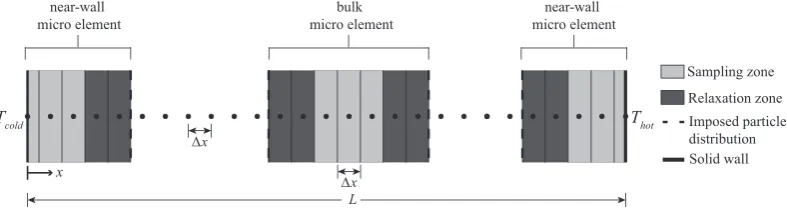
the temperature field across the system domain; as discussed in section 2.1, the flux-correction fieldΦwill automatically adjust for any error resulting from this assumption. Discretizing the domain in one-dimensional space, the macroscopic computational mesh consists ofN macro nodes, including a node at each wall. An example computa-tional domain set-up is shown in Fig. 2, where we have a micro element at each wall, and one in the bulk. This element arrangement is an example only — the appropriate arrangement will in practise depend on the case itself, as will be discussed further in section 3.2.1. For this 1D problem, each near-wall element comprises a single sampling zone and a single relaxation zone, while each bulk element consists of a single sampling zone with a relaxation zone on either side, as indicated in Fig. 2.

Each sampling zone is divided into a number of measurement bins. Similarly, each relaxation zone is divided into a number of control bins. In order to keep the transfer of data between the macroscopic mesh and the micro elements as simple as possible here, the bin arrangement in each element is set such that the centre of each bin coincides exactly with a macro node, i = 1, 2, ..., N. Again this is merely for convenience, and does not generally need to be imposed. The length of each 1D bin is then equal to the spacing between each macro node, ∆x.

Application of the general coupling algorithm of section 2.4 to this 1D system is as follows:

Sampling zone Relaxation zone Imposed particle distribution Solid wall

∆x

bulk micro element near-wall

micro element

near-wall micro element

∆x L

x

T

cold Thot

Figure 2: Schematic of the computational set-up for a one-dimensional Fourier flow problem.

(0) An initial estimate for the temperature field across the simulation domain is com-puted by solving the 1D conservation of energy equation,

dqx

dx = 0, (10)

whereqx is the streamwise component of the heat flux vector. This expression can

be closed using the 1D form of Fourier’s law,

qx=−κ

_dT dx

. (11)

Using the reference thermal conductivityκr, the 1D energy equation becomes,

κr

_d2_T

dx2

= 0, (12)

and can be approximated using a second order central finite difference scheme. With no temperature-jump at the solid walls (i.e. T1 = Tcold and TN = Thot),

solution results in the initial continuum temperature fieldTNSF.

(1) As the micro element size can change at each iteration (as will be discussed in section 3.2.1), each element is initialised at equilibrium before boundary condi-tions are applied. This is done by sampling particle velocities from a Maxwellian distribution. For consistency between the micro and macro domains, the tempera-ture and density for initialisation are obtained from the local continuum solution: continuum values of these properties are averaged over a sub-region of the macro domain that corresponds to the particular micro element.

Each micro element is then constrained:

(a) The local continuum temperature field is imposed throughout each relaxation zone by implementing a thermostat in each control bin.

(b) Maxwellian particle distributions are imposed at the outer boundaries of each relaxation zone via a diffuse solid wall condition at the local continuum tem-perature.

(2) DSMC is executed in each micro element. When steady-state conditions are reached, time averaging of properties is performed in each measurement bin. From each bin, time-averaged values of the temperature and the heat flux are extracted. Also, from both near-wall sampling zones, the temperature of the gas in contact with the bounding wall is extracted.

(3) Using the temperature and the heat flux extracted from each measurement bin, the flux-correction in each bin can be computed by applying the 1D flux-corrected constitutive relation with constant conductivityκr,

Φx=qx+κr

_dT dx

. (13)

For this calculation, the temperature gradient in each measurement bin is ap-proximated using a central finite difference scheme (or a forward/backward finite difference scheme for bins at the edges of the sampling zone). By computing the flux-correction in each measurement bin, the flux-correction field across each sam-pling zone is captured.

(4) To obtain Φxat every point in the domain, interpolation between sampling zones

is required. A study was performed showing that a simple linear interpolation provides an adequate representation of the full flux-correction field for this 1D case. Note that, for this 1D geometry, interpolation of the boundary gas temperature is not required.

(5) Using Eq. (13) to close Eq. (10) provides the 1D flux-corrected energy equation,

κr

_d2_T

dx2

−dΦx

dx = 0, (14)

which can be approximated using a second order central finite difference scheme. As discussed in section 2.3.2, temperature-jump boundary conditions are applied: the temperature of the gas at each bounding wall is set to be that measured in the corresponding near-wall element during Step (2). Solving this equation then results in the flux-corrected temperature fieldTΦacross the entire domain.

(6) Replacing the initial temperature field TNSF withTΦ, the process is repeated from

Step (1). This continues untilTΦconverges to within a user defined tolerance, i.e.

ζ= 1 N

N

X

i=1

TΦ(i)l−TΦ(i)l−1

TΦ(i)l

≤ζtol, (15)

where N is the number of macro nodes, l is the iteration index, and ζtol is the

tolerance parameter.

3.2. Results

The overall level of non-equilibrium in the gas is characterized here by a global Knud-sen numberKn, where the characteristic dimension is the separation between the heated wallsL, i.e.

Kn= λ

L. (16)

We use a Variable Hard Sphere (VHS) collision model in our DSMC simulations, and so the gas mean free path is given by [1],

λ=√ 1

2πd2_n, (17)

wheredis the VHS molecular diameter, andnis the number density of the gas. Localised regions of non-equilibrium can also result from large gradients in the macroscopic fluid properties, for example, temperature gradients. Varying bothKnand the temperature gradient across the system, we simulate a range of test cases here. These explore the ability of the hybrid method to deal with both missing constitutive and boundary in-formation, while remaining simple enough for validation against an equivalent full-scale DSMC simulation.

For simplicity, we simulate monatomic argon gas with the following VHS parameters: a reference temperature Tref = 273 K, a reference diameter dref = 4.17×10−10 m, and

viscosity exponentω = 0.81. For all test cases, the separation between the wallsL is 1 µm. In order to accurately capture the variation of the property fields, we set the number of macro nodesN across the domain to be 201 for all cases, making the constant spacing ∆xbetween each macro node 5nm. For each test case, we then set the gas density and the temperature of the walls to obtain the desiredKnand temperature gradient.

To ensure a fair comparison between each hybrid simulation and the equivalent full-scale DSMC simulation, we use the same cell-size and time-step in both the hybrid DSMC elements and the full-scale simulation. The cell size is set as a fraction of the gas mean free pathλ. The DSMC time-step must be a fraction of the mean collision time tmc:

a time-step ∆t = 1×10−12 s is sufficiently small for all cases simulated in this paper. In our testing, we found that an initial start-up run of 3 million time-steps allowed all DSMC simulations to reach steady state. To minimise the statistical scatter associated with the averaging of the field properties, all simulations were then run for a further 50 million time-steps.

As discussed in section 3.1, we monitor convergence of the hybrid procedure using Eq. (15), which quantifies the difference in the temperature solution between the current iteration and the previous. The tolerance parameter ζtol depends on the case itself,

with typical values of O(10−2_{) and below. We then require a measure of the overall}

accuracy for the converged hybrid solution when comparing with the corresponding full-scale DSMC solutionTFull. Here we consider the mean percentage error ¯in the hybrid

temperature profile, i.e.

¯ = 1

N

N

X

i=1

TFull(i)−TΦ(i)

TFull(i)

×100%. (18)

The value of this error depends on the hybrid’s ability to capture the ‘true’ flux-correction field across the simulation domain. The true flux-correction is that which can be com-puted from the full-scale DSMC solution Φx,Full, using the measured temperature field

TFull and the measured heat flux field qx,Fullin Eq. (13).

3.2.1. Micro resolution

The temperature-jump and associated thermal Knudsen layer are modelled within the micro element at each wall. To obtain a high level of accuracy for this Fourier flow

problem, the sampling zone in each of these elements should extend to capture the entire Knudsen layer. This means that the required size of our near-wall elements increases with the level of rarefaction, i.e.Kn. Note that, for high values ofKn, the required size of the near-wall micro elements may result in the hybrid approach (over a number of iterations) becoming less efficient than a full-scale DSMC treatment. For low values ofKn(where the Knudsen layers remain close to the walls), micro elements could be required in the bulk to capture non-equilibrium behaviour caused by strong temperature gradients. Even when the bulk of the domain is near-equilibrium, bulk micro elements may still be needed to provide a correction for any error in the assumed thermal conductivityκr. The micro

resolution (i.e the number of micro elements Π and their size) required for a particular problem is therefore dependent on both the level of rarefaction, and the temperature conditions.

To explore the effect of the micro element arrangement, we consider an example test case with Kn = 0.01. For a separation L = 1µm, we require a global mean free path λ = 0.01µm, corresponding to a gas number density n = 1.295×1026 _m−3 _from

Eq. (17). Setting an average gas temperatureTav = 273 K, we assume a value of κr =

0.0164 W/mK [32]. The temperature difference between the walls ∆T is set to 50 K (i.e. Tcold = 248 K and Thot = 298 K), resulting in a temperature gradient of 50×106 K/m

across the domain.

For this initial test case, with this Knudsen number and temperature gradient, the bulk of the domain will be in equilibrium. However, the flux-correction field Φx in the

bulk will be non-zero to correct for the assumption of a constant thermal conductivity. Over a temperature range of 200 K to 350 K, the thermal conductivity of argon varies approximately linearly with temperature, so Φx will also be approximately linear in the

bulk. Direct linear interpolation between the sampling zones of the near-wall elements should therefore provide an adequate representation of the full flux-correction field, and bulk micro elements are not needed for this initial case. Two near-wall elements should be sufficient, i.e. Π = 2.

Ideally, the sampling zones of these near-wall micro elements should capture the thermal Knudsen layers fully. Also, the relaxation zones must be large enough to allow full relaxation of the particle distribution. The size of both of these zones is therefore key to the accuracy of the hybrid method, and it is important that we are able to make an estimate of the appropriate size depending on the flow conditions. Typically, thermal Knudsen layers extend several mean free paths from a wall surface. Similarly, the relaxation of a particle state typically occurs over several mean free paths. We therefore express the extents of both the sampling and relaxation zones as some number of local mean free pathsλl.

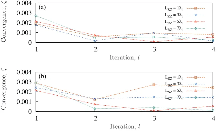
Two sensitivity studies have been performed to find the appropriate extent for each zone. In the first study, we keep the length of the sampling zoneLSZ at 5λland consider

the effect of the relaxation zone lengthLRZ by incrementally increasing its value from

1λl to 7λl. Then, in the second study, we consider the impact of LSZ by increasing it

from 1λl to 7λl, keeping LRZ constant at 5λl. Note that, for the first iteration, λl is

assumed equal to the global mean free path,λ =KnL. In subsequent iterations,λl is

updated for each micro element using Eq. (17), wheren is the average number density measured in the sampling zone of the element in the previous iteration.

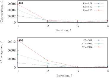
With elements in this size range, we need to see convergence of the hybrid method within 3 to 4 iterations for there to be any computational advantage over a full DSMC

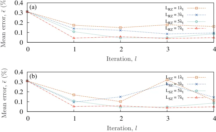
simulation. For this test case, we set the tolerance parameterζtolto be 0.001. Figure 3(a)

shows that, for all relaxation zone lengths, convergence of the method is reached within 4 iterations. However, convergence is not reached within 4 iterations when the sampling zone lengths are 1λl or 3λl, as shown in Fig. 3(b). We therefore require larger sampling

zones of either 5λl or 7λl, both of which provide convergence in only 2 to 3 iterations.

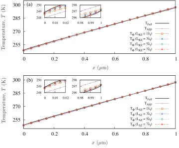
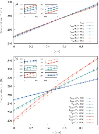
Note that, for all simulations, the level of convergence fluctuates slightly due to noise. The converged temperature profiles from the hybrid are shown in Fig. 4; also plotted is the initial temperature fieldTNSF, and the full DSMC temperature fieldTFull.

0

0.001

0.002

0.003

0.004

1

2

3

4

(a)

L_RZ = 3λ_l L_RZ = 5λ_l L_RZ = 7λ_l

0

0.001

0.002

0.003

0.004

1

2

3

4

(b)

L_SZ = 3λ_l L_SZ = 5λ_l L_SZ = 7λ_l

Figure 3: Convergence of the hybrid method for (a)LSZ = 5λland variousLRZ, and (b)LRZ = 5λl and variousLSZ.

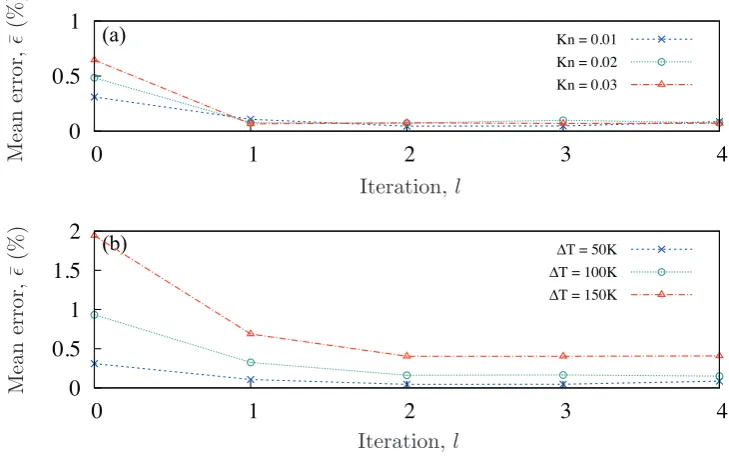
The accuracy of the hybrid method is, however, more apparent from the mean per-centage error at each iteration, presented in Fig. 5. The error at iterationl = 0 is the error in the initial hydrodynamic NSF solution. It is seen that the final mean error is less than 0.1% when relaxation and sampling zone extents are both 5λl or 7λl. This

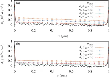
accuracy is due to the hybrid method’s ability to capture the flux-correction field across the domain, as shown in Fig. 6.

Essentially, the element size depends on the desired balance between accuracy and computational savings. Although sampling and relaxation zone extents of 7λl provide

slightly higher accuracy, we select an extent of 5λl for both zones. This provides a

sufficient level of accuracy while also enabling greater computational saving over a full-scale DSMC simulation. For the problems we study in this paper, each near-wall element therefore has a total extent of 10λl, while each bulk element has a total extent of 15λl.

255 270 285 300

0 0.2 0.4 0.6 0.8 1

(a)

T_Full T_NSF T_Φ (LRZ = 1λl)

T_Φ (L_RZ = 3λ_l) T_Φ (L_RZ = 5λ

l)

T_Φ (LRZ = 7λl)

255 270 285 300

0 0.2 0.4 0.6 0.8 1

(b)

T_Full TNSF

T_Φ (L_SZ = 1λ_l) T_Φ (L_SZ = 3λ

l)

T_Φ (LSZ = 5λl)

T_Φ (L_SZ = 7λ_l) 248

249 250

0 0.01 0.02

296 297 298

0.98 0.99 1

248 249 250

0 0.01 0.02

296 297 298

0.98 0.99 1

Figure 4: Final hybrid temperature solutionsTΦfor (a)LSZ = 5λland variousLRZ, and (b)LRZ = 5λland variousLSZ. These are compared to the corresponding full DSMC temperature solutionTFull,

and the hydrodynamic temperature solutionTNSF. Insets show results close to each wall.

3.2.2. Various rarefaction and temperature conditions

We now demonstrate the method’s ability to capture temperature jump and the associated thermal Knudsen layer under various rarefaction conditions (study A) and various temperature conditions (study B). In each test case, we maintain a wall separation L= 1µm, and an average gas temperatureTav = 273 K.

In study A, we consider the global Knudsen numbers: Kn = 0.01, 0.02, 0.03. This is achieved by varying the gas density for each case according to Eqs. (17) and (16). For all three cases, the temperature difference ∆T between the walls is set to 50 K. In study B, we simulate a range of temperature conditions by varying the temperature difference between the walls: ∆T = 50 K, 100 K, 150 K. For all three cases, the gas density is set to maintainKn= 0.01. For every test case considered, bothKnand the temperature gradient are small enough that the bulk of the domain will be in equilibrium. As in section 3.2.1, two near-wall elements should therefore be sufficient to capture the flux-correction field.

For all the cases, convergence of the hybrid solution occurs within 3 iterations to a tolerance parameter ofζtol= 0.001. This is shown in Figs. 7(a) and 7(b), for studies A and

0

0.1

0.2

0.3

0.4

0

1

2

3

4

(a)

L_RZ = 3λ_l L_RZ = 5λl

L_RZ = 7λ_l

0

0.1

0.2

0.3

0.4

0

1

2

3

4

(b)

L_SZ = 3λ_l L_SZ = 5λ_l L_SZ = 7λl

Figure 5: Mean error ¯in the hybrid solutions for (a)LSZ= 5λland variousLRZ, and (b)LRZ= 5λl and variousLSZ.

B, respectively. In Fig. 8(a), we present the converged temperature profiles from all three hybrid simulations of study A, along with the corresponding full DSMC temperature profiles. Also shown is the initial NSF temperature profile: as this is independent ofKn, it is the same for all test cases in study A. Similarly, the converged temperature profiles from all three hybrid simulations of study B are shown in Fig. 8(b). The corresponding full-scale DSMC and initial NSF temperature profiles are also shown, with the NSF solution different for each value of ∆T.

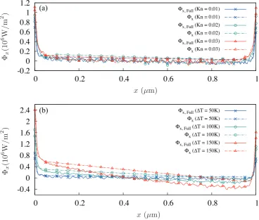
Again, a clearer measure of accuracy is to consider the mean percentage error of the hybrid solution (compared with the corresponding full DSMC solution) at each iteration. This is presented in Fig. 9 and, for each case, the error at iterationl = 0 represents the error in the initial NSF solution. For all three values of Kn in study A, the hybrid technique reduces ¯ to approximately 0.07% as shown in Fig. 9(a). Figure 10(a) shows that, for allKn, the final hybrid flux-correction representation is in fairly good agreement with the corresponding full DSMC flux-correction. However, as ∆T is increased in study B, Fig. 9(b) shows that the overall accuracy of the hybrid method decreases. This is a reflection of the lower quality of the hybrid flux-correction representation, as seen in Figure 10(b). However it should be noted that, for all values of ∆T, the hybrid solution provides a considerable improvement over the corresponding NSF solution.

For higher temperature gradients, the accuracy of the hybrid could be improved by slightly increasing the extent of the near-wall elements (i.e. largerLRZ andLSZ), or by

adding a element in the bulk. This would, however, reduce the computational savings obtained. As discussed in section 3.2.1, there must be a balance exercised between the accuracy required from, and the computational speed-up offered by, the hybrid method.

0

0.2

0.4

0.6

0.8

1

0

0.2

0.4

0.6

0.8

1

(a)

Φ_x (L_RZ = 1λ_l) Φ_x (L_RZ = 3λ_l) Φ_x (L_RZ = 5λ_l) Φ_x (L_RZ = 7λ_l)

0

0.2

0.4

0.6

0.8

1

0

0.2

0.4

0.6

0.8

1

(b)

Φ_x (L_SZ = 1λ_l) Φx (LSZ = 3λl)

Φx (LSZ = 5λl)

Φx (LSZ = 7λl)

Figure 6: Final hybrid flux-correction fields Φxfor (a)LSZ= 5λland variousLRZ, and (b)LRZ= 5λl and variousLSZ. These are compared with the full-scale DSMC flux-correction Φx,Full.

3.2.3. Extreme temperature conditions

For the cases in sections 3.2.1 and 3.2.2, we used only two near-wall elements in our hybrid approach. However, even if the bulk of the domain is near-equilibrium, higher temperature conditions might result in a non-linear variation of conductivity with temperature. If so, the use of linear interpolation of the flux-correction field between opposite near-wall elements is not likely to produce the most accurate solution. Accuracy should be improved by the addition of micro elements within the bulk, i.e. increasing the micro resolution.

To verify the method’s ability to deal with more extreme temperature conditions, we consider a case where the global Knudsen number is set to Kn= 0.01, but Tav is

increased to 500 K. The assumed value ofκris therefore increased to 0.027 W/mK [32].

The temperature difference ∆T between the walls is then set equal to 600 K (i.e.Tcold=

200 K andThot = 800 K). We consider two hybrid configurations: in the first, we have

only two near-wall elements, i.e. Π = 2; in the second, we add a bulk element in the centre of the system, i.e. Π = 3.

Settingζtol = 0.01 for this test case, convergence occurs within 3 iterations for both

configurations, as seen in Fig. 11. The converged temperature profiles from both hybrid simulations, along with the initial NSF and the full-scale DSMC temperature profiles, are presented in Fig. 12.

0

0.002

0.004

0.006

1

2

3

4

(a)

Kn = 0.02

Kn = 0.03

0

0.004

0.008

0.012

1

2

3

4

(b)

∆T = 100K

∆T = 150K

Figure 7: Convergence of the hybrid method for (a) variousKn(study A), and (b) various ∆T (study B).

centage error, shown for each iteration in Fig. 13. As we would expect, the addition of a bulk micro element results in a more accurate temperature solution. In fact, in com-parison with the initial NSF solution, this configuration provides an order of magnitude reduction in the mean error. This increased accuracy is the result of the higher quality flux-correction representation, as shown in Fig. 14.

The accuracy of the hybrid could be further improved by increasing the molecular resolution either by increasing the element lengths, or by adding more bulk elements, or both. It should be noted however that even with only two near-wall elements the hybrid solution still provides a considerable improvement over the NSF solution.

3.2.4. Computational savings

In this paper we have not exploited time-scale separation — the full-scale and the hybrid element simulations are run for the same number of DSMC time-steps. Compu-tational savings therefore come only from length-scale separation. The dimensions of the Fourier flow test cases considered here have been restricted by the need for a full-scale DSMC simulation in order to validate the hybrid method. With the degree of length-scale separation fairly small, the required micro elements occupy a significant portion of the domain. The computational savings provided by the hybrid on this particular heat transfer problem are therefore modest.

240 260 280 300

0 0.2 0.4 0.6 0.8 1 (a)

T

NSF

T

Full (Kn = 0.01)

T_Φ (Kn = 0.01) T_Full (Kn = 0.02) T_Φ (Kn = 0.02) T

Full (Kn = 0.03)

T_Φ (Kn = 0.03)

200 220 240 260 280 300 320 340

0 0.2 0.4 0.6 0.8 1 (b)

T_Full (∆T = 50K) T_NSF (∆T = 50K) T_Φ (∆T = 50K) T

Full (∆T = 100K)

T_NSF (∆T = 100K) T_Φ (∆T = 100K) T

Full (∆T = 150K)

T

NSF (∆T = 150K)

T_Φ (∆T = 150K)

248 250 252

0 0.02 294 296 298

0.98 1

200 204

0 0.02 224

228 248 252

296 300

0.98 1 320

324 344 348

Figure 8: Final hybrid temperature solutionsTΦ for (a) variousKn (study A), and (b) various ∆T

(study B). These are compared with the corresponding initial NSF temperature solutionsTNSF, and the

corresponding full DSMC temperature solutionsTFull. Insets show results close to each wall.

total processing time of the full DSMC approach, to the total processing time of the hybrid approach. For each simulation, the total processing time can be computed from the total number of DSMC time-stepsM ×the average clock time per DSMC time-step

0

0.5

1

0

1

2

3

4

(a)

Kn = 0.02

Kn = 0.03

0

0.5

1

1.5

2

0

1

2

3

4

(b)

∆T = 100K

∆T = 150K

Figure 9: Mean error ¯in the hybrid solutions for (a) variousKn(study A), and (b) various ∆T (study B).

tc, i.e.

S= MFulltc,Full MHybridtc,Hybrid

. (19)

Note thatM is the total number of time-steps over both the transient and steady-state periods and, for all cases in this paper,MHybrid =MFull = 53×106. The computational

cost of the hybrid approach depends on both the micro resolution, and the number of iterations required. As the physical extent of each element is updated after each iteration based on the local mean free path, the average clock time per time steptcfor a particular

element will differ for each iteration. The total average clock time per time-step for the hybrid approachtc,Hybrid is therefore calculated as the sum of tc for all micro elements

Π, over all iterationsI, i.e.

tc,Hybrid=

I

X

l=1

" Π

X

k=1

tc(k, l)

#

. (20)

For all test cases in section 3.2.2, our hybrid requires only two near-wall elements and convergence is reached inside 3 iterations. With Π = 2 and I = 3, the computational speed-upSis presented in Table 1 for each case. These speed-ups are determined by the extents of the near-wall subdomains, (LSZ +LRZ)left and (LSZ +LRZ)right which are

each 10λl. These extents during the final iteration (I= 3) of each case are also presented

in Table 1. IfKn= 0.01, (LSZ+LRZ)left and (LSZ+LRZ)right are small enough that

we see a modest computational speed-up (S > 1). However, when Knis increased to 0.02 and 0.03, these extents become larger so that we see no speed-up at all (S <1).

-0.2

0

0.2

0.4

0.6

0.8

1

1.2

0

0.2

0.4

0.6

0.8

1

(a)

Φx (Kn = 0.01)

Φx, Full (Kn = 0.02)

Φx (Kn = 0.02)

Φ_{x, Full} (Kn = 0.03) Φ_x (Kn = 0.03)

-0.4

0

0.4

0.8

1.2

1.6

2

2.4

0

0.2

0.4

0.6

0.8

1

(b)

Φ_x (∆T = 50K) Φx, Full (∆T = 100K)

Φx (∆T = 100K)

Φx, Full (∆T = 150K)

Φ_x (∆T = 150K)

Figure 10: Final hybrid flux-correction fields Φx for (a) variousKn (study A), and (b) various ∆T (study B), compared with the corresponding full DSMC flux-correction Φx,Full.

0

0.02

0.04

0.06

1

2

3

4

Π = 2

Π = 3

Figure 11: Convergence of the hybrid method for both Π = 2 and Π = 3 elements.

Convergence of the multiscale method is also reached inside 3 iterations for both element configurations considered in section 3.2.3, whereKn= 0.01 and ∆T = 600 K.

200

300

400

500

600

700

800

0

0.2

0.4

0.6

0.8

1

T_Full T_NSF T_Φ: Π = 2

T_Φ: Π = 3

200 220

0 0.01 0.02 780 800

0.98 0.99 1

Figure 12: Final hybrid temperature solutionsTΦ, along with the initial NSF temperature solutionTNSF,

and the full DSMC temperature solutionTFull. Insets show results close to each wall.

0

2

4

6

8

10

0

1

2

3

4

Π = 2

Π = 3

Figure 13: Mean error ¯for both hybrid configurations, Π = 2 and Π = 3.

-5

0

5

10

15

20

25

0

0.2

0.4

0.6

0.8

1

Φ_{x, Full} Φ_x: Π = 2 Φ_x: Π = 3

Figure 14: Final hybrid flux-correction fields Φx, and the full DSMC flux-correction field Φx,Full.

WithI = 3, the computational speed-ups for this case for both Π = 2 and Π = 3 are shown in Table 2. For the configuration with only near-wall elements, (LSZ +LRZ)left

and (LSZ+LRZ)rightare again small enough for us to see a modest computational

speed-up. However, the increase in accuracy that comes with the addition of the bulk element increases the computational cost. In fact, with a bulk element length (LSZ+ 2LRZ)bulk

corresponding to 15λl, there is no computational speed-up at all, andS <1.

Study A

Kngl ∆T (K) (LSZ+LRZ)left(µm) (LSZ+LRZ)right(µm) I S

0.01 50 0.1 0.1 3 1.77

0.02 50 0.19 0.21 3 0.88

0.03 50 0.29 0.31 3 0.59

Study B

0.01 50 0.1 0.1 3 1.77

0.01 100 0.09 0.11 3 1.73

0.01 150 0.09 0.11 3 1.77

Table 1: Computational speed-ups for the test cases of section 3.2.2.

Π (LSZ+LRZ)left (µm) (LSZ+ 2LRZ)bulk(µm) (LSZ+LRZ)right (µm) I S

2 0.07 - 0.12 3 1.71

3 0.07 0.15 0.12 3 0.96

Table 2: Computational speed-ups for the configurations of section 3.2.3.

In summary, while several cases in this paper demonstrate moderate computational savings by using the hybrid method, a number of cases are more computationally expen-sive than the equivalent full-scale DSMC simulation. It is important to note, however, that these Fourier flow cases have been chosen simply to test and validate the hybrid methodology itself. Future simulations of larger, more realistic, 2D and 3D problems will highlight any computational advantages of our multiscale approach. In transient flows, when temporal variations in the macroscopic property fields are much slower than the molecular time scales, computational savings can also be obtained by exploiting time scale separation, i.e. by controlling the time-steps in the macro and micro models as described by Lockerbyet al.[33].

4. Conclusions

Based on a HMM-FWC approach, we have proposed a hybrid multiscale method that couples a continuum-fluid solver with the DSMC particle technique. The key advantage of this hybrid over existing continuum-DSMC hybrids is that DSMC micro elements of any size can be placed at any location in the flow, i.e. close to walls or in the bulk of the domain, independent of the continuum description. Therefore, unlike traditional HMM techniques, our method is able to simulate problems with any degree of scale separation. The micro resolution can be adjusted for each problem to obtain the desired balance

between accuracy and computational cost. Another useful feature of our approach is that the size of the micro elements adapts dynamically depending on the local mean free path of the gas.

For heat-transfer problems, the coupling in our method is performed through the computed heat fluxes. As a simple validation test, the method was demonstrated on micro Fourier flow. For a range of rarefaction and temperature conditions, we have shown the method’s ability to compensate for inaccurate boundary and constitutive information. The hybrid procedure was found to converge very quickly, inside 3 iterations for all test cases considered. Generally, good agreement with the equivalent full-scale DSMC simulations was observed, with the exact level of accuracy depending on the micro element arrangement.

Due to the small degree of scale separation in the Fourier flow cases considered here, the computational speed-ups observed (over the full DSMC simulations) were modest. This problem was, however, selected only to provide a simple example on which to test and validate the underlying methodology. Much greater speed-ups can be expected when simulating larger, more realistic engineering problems.

Before tackling 2D and 3D problems, the method needs to be developed to enable full coupling of mass and momentum, as well as heat transfer. Extension to 2D/3D then presents some additional challenges, including the application of mass, momentum, and heat transfer boundary conditions within 2D/3D relaxation zones, and 2D/3D interpola-tion of the flux-correcinterpola-tion field between sampling zones. However, with this development, the method has the potential to tackle a variety of problems, such as the flow of com-plex gas mixtures, or the flow through micro heat exchangers. The modelling of thin bow shockwaves at the front of a planetary re-entry vehicle is another example which could benefit from the development of this hybrid as it encompasses both complex fluid behaviour (including chemical reactions of many gas species) and a high aspect ratio geometry. Our method also has the potential to be used in an inverse manner to obtain the transport properties of a gas.

5. Acknowledgements

This work is financially supported in the UK by EPSRC Programme Grant EP/I011927/1. Results were obtained using the ARCHIE-WeSt High Performance Computer (www.archie-west.ac.uk) at the University of Strathclyde, funded by EPSRC grant EP/K000586/1. SYD would like to thank Craig White and Alexander Patronis for their help and advice. The authors would also like to thank the reviewers of this paper for their very helpful comments.

References

[1] G. A. Bird, Molecular Gas Dynamics and the Direct Simulation of Gas Flows, Oxford Engineering Science Series, Clarendon Press, 1998.

[2] S. T. O’Connell, P. A. Thompson, Molecular dynamics - continuum hybrid computations: A tool for studying complex fluid flows, Physical Review E 52 (1995) R5792–R5795.

[3] N. G. Hadjiconstantinou, A. T. Patera, Heterogeneous atomistic-continuum representations for dense fluid systems, International Journal of Modern Physics C 8 (4) (1997) 967–976.

[4] E. G. Flekkøy, G. Wagner, J. Feder, Hybrid model for combined particle and continuum dynamics, Europhysics Letters 52 (3) (2000) 271.

[5] R. Delgado-Buscalioni, P. V. Coveney, Continuum-particle hybrid coupling for mass, momentum, and energy transfers in unsteady fluid flow, Physical Review E 67 (2003) 046704.

[6] T. Werder, J. H. Walther, P. Koumoutsakos, Hybrid atomistic-continuum method for the simulation of dense fluid flows, Journal of Computational Physics 205 (1) (2005) 373–390.

[7] D. C. Wadsworth, D. A. Erwin, One-dimensional hybrid continuum/particle simulation approach for rarefied hypersonic flows, Proceedings of the 5th AIAA/ASME Joint Thermophysics and Heat Transfer Conference, Seattle, WA.

[8] D. B. Hash, H. A. Hassan, Assessment of schemes for coupling Monte Carlo and Navier-Stokes solution methods, Journal of Thermophysics and Heat Transfer 10 (2) (1996) 242–249.

[9] A. L. Garcia, J. B. Bell, W. Y. Crutchfield, B. J. Alder, Adaptive mesh and algorithm refinement using Direct Simulation Monte Carlo, Journal of Computational Physics 154 (1) (1999) 134–155. [10] O. Aktas, N. R. Aluru, A combined continuum/DSMC technique for multiscale analysis of

microflu-idic filters, Journal of Computational Physics 178 (2) (2002) 342–372.

[11] R. Roveda, D. B. Goldstein, P. L. Varghese, Hybrid Euler/particle approach for continuum/rarefied flows, Journal of Spacecraft and Rockets 35 (1998) 258–265.

[12] Q. Sun, I. D. Boyd, G. V. Candler, A hybrid continuum/particle approach for modeling subsonic, rarefied gas flows, Journal of Computational Physics 194 (1) (2004) 256–277.

[13] Q. Sun, I. D. Boyd, A direct simulation method for subsonic, microscale gas flows, Journal of Computational Physics 179 (2) (2002) 400–425.

[14] H. S. Wijesinghe, R. D. Hornung, A. L. Garcia, N. G. Hadjiconstantinou, Three-dimensional hy-brid continuum-atomistic simulations for multiscale hydrodynamics, Journal of Fluids Engineering 126 (5) (2004) 768–777.

[15] J.-S. Wu, Y.-Y. Lian, G. Cheng, R. P. Koomullil, K. C. Tseng, Development and verification of a coupled DSMC–NS scheme using unstructured mesh, Journal of Computational Physics 219 (2) (2006) 579–607.

[16] T. Schwartzentruber, L. Scalabrin, I. Boyd, A modular particle–continuum numerical method for hypersonic non-equilibrium gas flows, Journal of Computational Physics 225 (1) (2007) 1159–1174. [17] Y.-Y. Lian, K.-C. Tseng, Y.-S. Chen, M.-Z. Wu, J.-S. Wu, G. Cheng, An improved parallelized hybrid DSMC-NS algorithm, Proceedings of the 26th International Symposium on Rarefied Gas Dynamics, Kyoto, Japan 1084 (1) (2008) 341–346.

[18] W. Ren, W. E, Heterogeneous multiscale method for the modeling of complex fluids and micro-fluidics, Journal of Computational Physics 204 (1) (2005) 1–26.

[19] S. Yasuda, R. Yamamoto, A model for hybrid simulations of molecular dynamics and computational fluid dynamics, Physics of Fluids 20 (11) (2008) 113101.

[20] N. Asproulis, M. Kalweit, D. Drikakis, A hybrid molecular continuum method using point wise coupling, Advances in Engineering Software 46 (1) (2012) 85–92.

[21] M. K. Borg, D. A. Lockerby, J. M. Reese, A multiscale method for micro/nano flows of high aspect ratio, Journal of Computational Physics 233 (2013) 400–413.

[22] D. A. Kessler, E. S. Oran, C. R. Kaplan, Towards the development of a multiscale, multiphysics method for the simulation of rarefied gas flows, Journal of Fluid Mechanics 661 (2010) 262–293. [23] A. Patronis, D. A. Lockerby, M. K. Borg, J. M. Reese, Hybrid continuum–molecular modelling of

multiscale internal gas flows, Journal of Computational Physics 255 (2013) 558–571.

[24] M. K. Borg, D. A. Lockerby, J. M. Reese, Fluid simulations with atomistic resolution: a hybrid multiscale method with field-wise coupling, Journal of Computational Physics 255 (2013) 149 – 165. [25] M. von Smoluchowski, Ueber w¨armeleitung in verd¨unnten gasen, Annalen der Physik 300 (1) (1898)

101–130.

[26] OpenFOAM Foundation, www.openfoam.org (2013). URLwww.openfoam.org

[27] T. J. Scanlon, E. Roohi, C. White, M. Darbandi, J. M. Reese, An open source, parallel DSMC code for rarefied gas flows in arbitrary geometries, Computers & Fluids 39 (10) (2010) 2078–2089. [28] E. Arlemark, G. Markelov, S. Nedea, Rebuilding of Rothe’s nozzle measurements with OpenFOAM

software, Journal of Physics: Conference Series 362 (1) (2012) 012040.

[29] C. White, M. K. Borg, T. J. Scanlon, J. M. Reese, A DSMC investigation of gas flows in micro-channels with bends, Computers & Fluids 71 (2013) 261–271.

[30] M. K. Borg, G. B. Macpherson, J. M. Reese, Controllers for imposing continuum-to-molecular boundary conditions in arbitrary fluid flow geometries, Molecular Simulation 36 (10) (2010) 745– 757.

[31] A. J. Lofthouse, Nonequilibrium hypersonic aerothermodynamics using the direct simulation monte carlo and navier-stokes models, Ph.D. thesis, University of Michigan (2008).

[32] B. A. Younglove, H. J. M. Hanley, The viscosity and thermal conductivity coefficients of gaseous and liquid argon, Journal of Physical and Chemical Reference Data 15 (1986) 1323–1337. [33] D. A. Lockerby, C. A. Duque-Daza, M. K. Borg, J. M. Reese, Time-step coupling for hybrid

simu-lations of multiscale flows, Journal of Computational Physics 237 (2013) 344 – 365.