SFB
823
growth in the EU: A recursive
partitioning approach
Discussion Paper
Martin Wagner, Achim Zeileis
Nr. 80/2016
EU: A Recursive Partitioning Approach
Martin Wagner
Technical University Dortmund Institute for Advanced Studies, Vienna
Bank of Slovenia, Ljubljana
Achim Zeileis
Universität Innsbruck
Abstract
We use model-based recursive partitioning as a technique to assess heterogeneity of growth and convergence processes based on an economic growth regression for 255 European Union NUTS2 regions from 1995 to 2005. The starting point of the analysis is a human-capital-augmented Solow-type growth equation similar in spirit toMankiw, Romer, and Weil (1992). Initial GDP and the share of highly educated in the working age population are found to be important for explaining economic growth, whereas the investment share in physical capital is only significant for coastal regions in the PIIGS countries. Recursive partitioning leads to a regression tree with four terminal nodes with partitioning according to (i) capital regions, (ii) non-capital regions in or outside the so-called PIIGS countries and (iii) inside the respective PIIGS regions furthermore between coastal and non-coastal regions.
Keywords: convergence, growth regressions, recursive partitioning, regional data. JEL classification: C31, C51, O18, O47.
1. Introduction
The econometric analysis of the determinants of economic growth and of potential conver-gence of output across countries or regions has been a major research topic in economics in the last decades. Early empirical contributions include Baumol (1986),Barro(1991) or
Barro and Sala-i-Martin (1992). Since then in numerous studies – that employ a broad
variety of methods – a large number of potential explanatory variables has been considered, for an overview see Durlauf, Johnson, and Temple (2005).
Given the open-endedness of economic growth theories, in the words ofBrock and Durlauf
(2001), a key question is to determine, out of an often large set of candidate variables, the variables relevant for economic growth. To address this uncertainty many contributions have applied some form of model averaging, be it Bayesian (e.g., Doppelhofer, Crespo
Sala-i-Martin, Doppelhofer, and Miller 2004) or frequentist (e.g., Hlouskova and Wagner
2013;Wagner and Hlouskova 2015). The latter two papers combine model averaging
tech-niques with principal components augmentation to achieve regularization and complexity reduction. Schneider and Wagner(2012) use the adaptive LASSO estimator, that simulta-neously performs model selection and parameter estimation, to single out the determinants of economic growth in the regions of the European Union (EU).
All the mentioned contributions assume, however, that the relationship between economic growth and the explanatory variables is identical for all considered countries or regions. This assumption is clearly restrictive given the large theoretical literature that implies that growth processes across countries or regions are not necessarily governed by a common linear relationship, compare Azariadis and Drazen (1990); Durlauf (1993) and Murphy,
Shleifer, and Vishny (1989). These models highlight different mechanisms that may lead
to potential nonlinearities in growth processes, e.g., poverty traps or convergence clubs. Furthermore, the usually considered data sets that comprise very heterogeneous countries or regions make the assumption of a common growth process, even when controlling for a variety of variables, at least worth investigating.
The present paper assesses the homogeneity of the growth process by using model-based recursive partitioning for a data set covering the 255 NUTS2 regions of the EU from 1995 to 2005. The approach draws on the rich economic growth literature in two ways: First, a basic and economically interpretable regression model is selected using a human-capital-augmented Solow-type growth equation similar in spirit to Mankiw et al. (1992). Second,
the regression is assessed and split recursively along variables that have previously been em-ployed in studies of potential heterogeneities and nonlinearities of growth and convergence phenomena (especially in the EU). Moreover, recursive partitioning of growth regressions to uncover multiple regimes has been considered previously byDurlauf and Johnson(1995). They employ a recursive partitioning algorithm that combines the classification and regres-sion tree (CART) approach ofBreiman, Friedman, Olshen, and Stone (1984) with residual sums of squares from growth regressions. However, while that approach lacks a concept of (asymptotic) significance of the regimes found, we use a modern model-based extension of the classic recursive partitioning approaches suggested by Zeileis, Hothorn, and Hornik
(2008) based on formal (score-based) parameter stability tests.
The regression and recursive partitioning methods are presented in Section 2 before Sec-tion 3 introduces the details of the data and variables considered. The results of the analysis are discussed in Section 4and Section 5concludes.
2. Method
As will be discussed and motivated in more detail in Section 3, the growth regression considered is a human-capital-augmented Solow-type model:
yi = β0 +xi1β1+· · ·+xi4β4+εi (1)
for our sample ofi= 1, . . . ,255 EU regions with the dependent variable y= (y1, . . . , yn)>,
the annual growth rate of real GDP per capita over 1995–2005 (‘ggdpcap’),x1 = (x11, . . . , xn1)>
the logarithm of initial GDP in 1995 (‘gdpcap0’), x2 = (x12, . . . , xn2)> the share of gross
fixed capital formation (’shgfcf’), x3 = (x13, . . . , xn3)> and x4 = (x14, . . . , xn4)> the shares
of highly and medium educated population (‘shsh’ and ‘shsm’). As usual,ε = (ε1, . . . , εn)0
denotes the error vector. Parameter estimation is performed by ordinary least squares (OLS).
To assess whether the parameter vector β in (1) is in fact stable over all 255 observations,
the model is partitioned as proposed in Zeileis et al. (2008). To do so, we iterate between
(a) estimating the parameters of (1) in the given (sub)sample by OLS and (b) in case of evidence for non-stable β-coefficients splitting the data set into two subsamples. For
step (b) additional ‘partitioning’ variables are employed with respect to which parameter stability is first assessed and, if any is found, the best split in subsamples is selected by minimizing the residual sum of squares of the partitioned model.
The parameter instability tests considered have first been suggested in the context of time series regressions but can also be applied to other contexts (e.g., Hjort and Koning 2002;
Zeileis and Hothorn 2013). More specifically, the stability of the regression coefficients is
tested using the supLM test of Andrews(1993) for numerical partitioning variables:
supLM = sup i=i,...,ı i n 1− i n −1 ˆ V−1/2n−1/2 X `:z`≤z(i) x`•εˆ` 2 2 , (2)
where zi denotes observation i of the considered partitioning variable, after ordering
ac-cording to increasing size denoted by z(i). Furthermore, ˆε is the vector of OLS residuals;
based on parameter estimation on the considered (sub)sample. ˆV =n−1Pn
i=1εˆ2ixi•x>i•is the
outer-product-of-gradients (OPG) covariance estimate, employed to normalize the sums of the score vectors xi•εˆi.
For categorical partitioning variables the test statistic is given by:
χ2 = X c=1,...,C ˆ V−1/2n−c1/2 X i:zi=c xi•εˆi 2 2 , (3)
denoting here with c = 1, . . . , C the categories of the partitioning variable z and with nc
the number of observations of z in category c.
Asymptoticp-values for both tests can be computed from the corresponding limiting
distri-butions: supremum of a squared tied-down Bessel process for the supLM-test (seeHansen 1997) and chi-squared with 5×(C−1) degrees of freedom for theχ2-test, respectively. See
Hjort and Koning (2002) and Zeileis (2005) for a unifying view and further discussions of
these parameter stability tests. Additionally, we apply a Bonferroni-type correction to the
p-values to correct for testing along several (and not just a single) partitioning variable.
The recursive partitioning procedure stops if no more significant instability is detected (at the 5% level) or the subsample becomes too small (less than twelve observations in our
application). In each of the resulting subsamples or ‘groups of regions’ the basic Solow-type model above is fitted. Consequently, we model growth and convergence for EU regions as linear, but with different coefficients for different ‘groups of regions’.1
3. Data
The data used in this paper are a subset of the variables used in Schneider and Wagner
(2012), see Table 1 for a list of variables. The regional dataset covers the 255 NUTS2 regions in the 27 member countries (at the time) of the EU over the period 1995–2005. The selection of variables used here from the larger dataset available is based on the fol-lowing considerations. First, as already discussed above, the basis of our model-based recursive partitioning approach is a simple, economically interpretable relationship. Sec-ond, as partitioning variables we consider variables according to which partitioning and heterogeneity appears to be a potential issue, given growth theory, the institutional and historical characteristics present in the EU, and the available empirical evidence. Third, the number of partitioning variables is limited by the need for having a sufficient set of
1Note that this strategy bears some resemblance to the approach of Crespo Cuaresma, Foster, and
Stehrer(2011). However, whilst they ‘partition’ according to quantiles of the distribution of thedependent
variable, our partitioning is related to a set ofindependent partitioning variables.
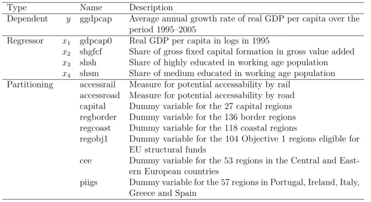
Type Name Description
Dependent y ggdpcap Average annual growth rate of real GDP per capita over the
period 1995–2005
Regressor x1 gdpcap0 Real GDP per capita in logs in 1995
x2 shgfcf Share of gross fixed capital formation in gross value added
x3 shsh Share of highly educated in working age population
x4 shsm Share of medium educated in working age population
Partitioning accessrail Measure for potential accessability by rail accessroad Measure for potential accessability by road capital Dummy variable for the 27 capital regions regborder Dummy variable for the 136 border regions regcoast Dummy variable for the 118 coastal regions
regobj1 Dummy variable for the 104 Objective 1 regions eligible for EU structural funds
cee Dummy variable for the 53 regions in the Central and East-ern European countries
piigs Dummy variable for the 57 regions in Portugal, Ireland, Italy, Greece and Spain
Table 1: List of variables. For a more detailed description including the sources see
Schnei-der and Wagner (2012). Note that the variable gdpcap0 is used not only as regressor but
observations in each (terminal) node. Fourth, we build in the analysis to a certain extent on the findings of Schneider and Wagner (2012) and Wagner and Hlouskova (2015) who use the same dataset.2
The dependent variable y is the average growth rate of real GDP per capita (ggdpcap)
and the regressors are initial real GDP per capita in logs (gdpcap0, x1) to capture
poten-tial β-convergence, the investment share in GDP (shgfcf, x2) to capture physical capital
accumulation and the shares of high and of medium educated in the labor force (shsh and shsm, x3 and x4) as measures of human capital. Thus, in effect we estimate a
human-capital-augmented version of the Solow model, inspired by the by now classical work of
Mankiw et al. (1992).
We employ the following partitioning variables:
• First, we use the log of initial real GDP per capita as a partitioning variable as a sim-ple device to check for the presence of convergence clubs. The important role of initial real GDP per capita in shaping growth and convergence dynamics in the form of, e.g., convergence clubs has been documented in many papers dealing with EU regions including Azomahou, El Ouardighi, Nguyen-Van, and Pham (2011), Basile (2008),
Firgo and Huber (2014),Fotopoulos (2012), orPetrakos, Kallioras, and Anagnostou
(2011).
• We use two measures for traffic accessibility of the region, one for accessibility via rail (accessrail) and one via the road network (accessroad). Clearly, integration in the European traffic networks is beneficial for trade and thus for economic development and growth. This variable has been found important, e.g., in Sanso-Navarro and
Vera-Cabello (2015).
• A dummy variable for capital regions (capital) is used. This variable has been found significant in Schneider and Wagner(2012), in line with the large literature on core-periphery effects in new economic geography models (compareFujita, Krugman, and
Venables 1999). For additional empirical evidence highlighting the importance of
agglomeration effects in the EU seeGeppert and Stephan (2008).
• We also consider dummy variables for border regions (regborder) and coastal regions (regcoast). Both of these variables are related to trade (and its impact on economic growth). Since the seminal study of McCallum (1995) that has investigated the detrimental effect of national borders on trade in North America such border effects have been found important in many empirical trade studies. Matters are ex ante less clear with respect to coastal regions since these are faced on the one hand with a ‘border’ with the sea but are for exactly that reason on the other hand (at least partly) the locations of ports. From this perspective coastal regions are expected to benefit from both EU imports and exports as well as from infrastructure investments.
2It has to be noted, however, that at the regional level the availability of core economic data is still
• A key tool of EU policy is to foster regional development via its structural funds, with the prime recipients of such funds being the so-called Objective 1 regions (regobj1). We include the corresponding dummy variable to assess the potential effects of EU structural funds on the regional growth performance (compare also Lall and Yilmaz
2001).
• Finally, we include two dummy variables corresponding to two different groups of countries. One is a CEE dummy for ten Central and Eastern European countries (i.e., Bulgaria, Czech Republic, Estonia, Hungary, Lithuania, Latvia, Poland, Roma-nia, Slovak Republic, and Slovenia) and the other is for the so-called PIIGS countries (Portugal, Ireland, Italy, Greece, and Spain). The former group comprises previously centrally planned economies that have joined the EU at the very end (May 1, 2004) or even after the sample period (January 1, 2007 in case of Bulgaria and Romania). Against this background (central planning legacy, recent EU membership) it sounds reasonable to at least check for whether the regions in these countries have experi-enced a different growth performance over our sample period. Details concerning the specificities of the growth process of these countries as well as growth projections are contained inWagner and Hlouskova (2005). The latter group comprises Southern or Western peripheral countries that have experienced a substantial crisis in the after-math of the global financial crisis. These are considered separately in order to see whether the growth performance in these regions has been different already prior to the crisis. The differential growth and convergence performance of the PIIGS coun-tries already prior to the crisis is, e.g., documented in Ertur, Le Gallo, and Baumont
(2006).
4. Results
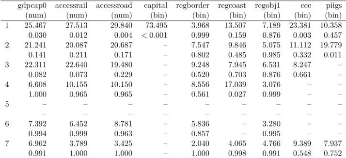
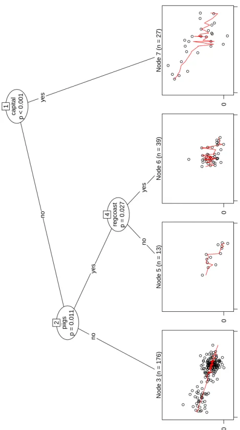
The results of the parameter stability tests are displayed in Table2. The results show that the regression tree is spanned (when the significance level is chosen to be 5%) with three partitioning variables (capital, piigs, and regcoast) and four terminal nodes, see Figure 1
for a visualization. According to these results capital regions indeed exhibit a different growth performance, as is true also for the PIIGS regions as well as coastal regions within the PIIGS countries. Note, however, that in the first block-row of Table2also for four more variables the null hypothesis of parameter stability is rejected at the 5% level (withp-values
higher than that of capital). These are initial GDP, the two accessibility measures, and the CEE dummy. Thus, viewed in isolation there is indeed evidence for heterogeneity along these variables. Nevertheless, after partitioning according to the capital region dummy, none of these variables reappears as a variable indicating associated heterogeneity. E.g., the finding with respect to the CEE dummy, not being significant as partitioning variable after partitioning according to the capital region dummy, is in line with the fact that for many of the CEE countries the bulk of growth has occurred in the capital region. After separating the sample between capital and non-capital regions there is no evidence for
gdpcap0 accessrail accessroad capital regborder regcoast regobj1 cee piigs (num) (num) (num) (bin) (bin) (bin) (bin) (bin) (bin) 1 25.467 27.513 29.840 73.495 3.968 13.507 7.189 23.381 10.358 0.030 0.012 0.004 <0.001 0.999 0.159 0.876 0.003 0.457 2 21.241 20.087 20.687 – 7.547 9.846 5.075 11.112 19.779 0.141 0.211 0.171 – 0.802 0.485 0.985 0.332 0.011 3 22.311 22.640 19.480 – 9.248 7.945 6.531 8.247 – 0.082 0.073 0.229 – 0.520 0.703 0.876 0.661 – 4 6.608 10.155 10.150 – 8.556 17.039 3.076 – – 1.000 0.965 0.965 – 0.561 0.027 0.999 – – 5 – – – – – – – – – – – – – – – – – – 6 7.392 6.452 8.781 – 5.836 – 3.280 – – 0.994 0.999 0.963 – 0.857 – 0.995 – – 7 6.962 3.789 3.425 – 2.040 4.065 4.766 9.389 7.937 0.991 1.000 1.000 – 1.000 0.998 0.991 0.548 0.752
Table 2: Parameter stability tests (test statistic and p-value) for all partitioning variables
in each of the tree’s nodes. For numerical variables (num) theAndrews(1993) supLM test
is used and for binary variables (bin) a score-based χ2 test.
initial income driven convergence clubs at the 5% significance level. Note, however, that in the terminal node of non-capital non-PIIGS regions that comprises a bulk of 176 regions there is some evidence for parameter instability at the 10% level. This can also be seen in the lower left graph of Figure 1, where a ‘blurred’ separation in two clusters – grouped according to initial output – is visible. Thus, at the 10% significance level there is evidence for two initial GDP driven convergence clubs in the non-capital non-PIIGS regions.3
There is no evidence for border effects in the sense of differing growth performance of border regions. This result can be tentatively interpreted as indicating that the European common market policies have been successful in removing trade barriers across EU member states. On the other hand it also appears that being an Objective 1 region does not lead to a differential growth process, which is in line with some of the literature that finds hardly any growth promoting effect of EU structural funds; for an early assessment see Canova
and Marcet (1997).
The second partitioning occurs with respect to the PIIGS dummy within the non-capital regions and the third with respect to coastal regions within the non-capital PIIGS regions. A graphical illustration of the regression tree is given by Figure 1.
3At the 10% significance level there is also evidence against parameter stability in this set of regions
when partitioning according to accessrail (in addition to the discussed instability with respect to initial GDP). If one were to enforce a split according to the logarithm of initial real GDP per capita, the split point is 9.712. The estimation results between the corresponding two subsets differ substantially in that only in the high initial income regions gross fixed capital formation and the share of highly educated in the labor force are significant with positive coefficients.
capital p < 0.001 1 no y es piigs p = 0.011 2 no y es Node 3 (n = 176) ● ● ● ● ● ● ●● ● ● ● ● ● ● ● ● ● ● ● ● ● ● ● ● ●●●●● ● ●● ● ● ● ●● ● ● ●● ● ● ● ● ● ●● ● ● ● ● ● ● ● ● ● ● ● ● ● ● ● ● ● ● ● ● ● ● ● ● ● ● ● ● ●● ● ● ● ● ● ● ●●●● ● ● ● ● ● ● ● ● ● ● ● ● ● ● ● ● ● ● ● ● ● ● ● ● ● ● ● ●● ● ● ●●●● ● ● ● ● ● ● ● ● ● ● ● ● ●●●● ● ● ● ● ● ● ● ● ● ● ● ● ● ●● ● ● ● ● ● ● ● ● ● ● ● ● ● ● ● ● ● ● ●● ● ● 8.1 10.9 0 regcoast p = 0.027 4 no y es Node 5 (n = 13) ● ● ● ● ● ● ● ● ● ● ●● ● 8.1 10.9 0 Node 6 (n = 39) ●● ● ● ● ● ● ●● ● ● ● ● ● ● ● ● ● ● ● ● ● ● ●● ● ● ● ● ●● ● ● ● ● ● ● ● ● 8.1 10.9 0 Node 7 (n = 27) ● ● ● ● ● ● ● ● ● ● ● ● ● ● ● ● ● ● ● ● ● ● ● ● ● ● ● 8.1 10.9 0
Figure 1: Fitted linear regression tree. In the inner nodes the p-values from the
param-eter stability tests are displayed and in terminal nodes a scatter plot of GDP per capita growth (ggdpcap) vs. (log) initial real GDP per capita (ggdcap0) along with fitted values is depicted.
Summary Partitioning variables Regressor variables
n R2 capital piigs regcoast (Const.) gdpcap0 shgfcf shsh shsm 3 176 0.505 no no – 0.166 −0.0159 −0.0030 0.024 0.0070 (0.013) (0.0014) (0.0071) (0.010) (0.0063) 5 13 0.923 no yes no 0.199 −0.0186 −0.0379 0.090 −0.0195 (0.067) (0.0071) (0.0426) (0.031) (0.0345) 6 39 0.560 no yes yes 0.120 −0.0139 0.0840 0.121 0.0089 (0.054) (0.0056) (0.0401) (0.028) (0.0208) 7 27 0.620 yes – – 0.240 −0.0242 −0.0034 0.045 0.0563 (0.063) (0.0058) (0.0527) (0.041) (0.0238)
Table 3: Fitted linear regression models for terminal nodes in the tree. Summary informa-tion (number of observainforma-tionsn and R2), the partitioning variables selected and regression
coefficients (with standard errors in brackets) are provided.
Let us now turn to the regression results given in Table 3. The table shows the results for the four terminal nodes shown also in Figure 1. For all four partitioned sets of regions, the coefficient to (log) initial real GDP per capita is negative, with the largest negative coefficient (and thus the highest associated conditionalβ-convergence speed) obtained for
the 27 capital regions. The lowest convergence speed prevails for the coastal regions in the PIIGS countries, in line with the above discussion concerning the versatile border and trade effects experienced by border/coastal regions. Whilst the impact of highly skilled in the working age population on growth is ubiquitously positive, it is negative (albeit not significant) for the 13 regions in the PIIGS countries that are not coastal. Surprisingly the investment share has a negative coefficient for all but the coastal PIIGS regions. However, it is only significant for this latter of the four groups of regions. Thus, in effect initial GDP and the share of highly skilled in the working age population are the two variables that are significant for all four groups of regions with coefficient signs in line with economic theory.
5. Summary
The paper demonstrates that the growth process in the 255 NUTS2 regions of the European Union is heterogeneous across four groups of regions. Loosening up the constraint of a single homogenous linear growth equation for all regions leads to a good description of the growth process by a simple human-capital-augmented Solow-type equation in the spirit ofMankiw
et al. (1992). The model-based recursive partitioning procedure singles out being a capital
region as most important partitioning variable, for which the null hypothesis of parameter stability is rejected with smaller p-value than for initial real GDP per capita, accessibility
measures or the CEE dummy variable. Amongst the non-capital regions partitioning occurs according to whether the region is in a so-called PIIGS country and within those whether it is a coastal region or not. The coastal regions in the PIIGS countries have the lowest conditional β-convergence speed. The results indicate that allowing for heterogeneity in
Moreover, the application highlights how model-based recursive partitioning may com-plement the econometric toolbox of empirical growth researchers: By combining well-established ‘standard’ models (the human-capital-augmented Solow-type equation in our case) with knowledge about further potential factors whose precise effects on economic growth are not clear ex ante, groups and interaction effects can be revealed. While the technique is exploratory in spirit, it is based on formal inference for parameter stabil-ity, thus controlling its significance level. Aided by the tree visualization, the results are furthermore straightforwardly and easily interpreted.
Acknowledgements
The first author gratefully acknowledges financial support from the Collaborative Research Center 823: Statistical Modelling of Nonlinear Dynamic Processesand from the
Jubiläums-fonds of the Oesterreichische Nationalbank via several grants. The usual disclaimer applies.
References
Andrews DWK (1993). “Tests for Parameter Instability and Structural Change with Un-known Change Point.” Econometrica, 61, 821–856. doi:10.2307/2951764.
Azariadis C, Drazen A (1990). “Threshold Externalities in Economic Development.” Quar-terly Journal of Economics, 105, 501–526. doi:10.2307/2937797.
Azomahou TT, El Ouardighi J, Nguyen-Van P, Pham TKC (2011). “Testing Convergence of European Regions: A Semiparametric Approach.” Economic Modelling, 28, 1202–
1210. doi:10.1016/j.econmod.2010.12.010.
Barro RJ (1991). “Economic Growth in a Cross-Section of Countries.” Quarterly Journal of Economics, 106, 407–445. doi:10.2307/2937943.
Barro RJ, Sala-i-Martin X (1992). “Convergence.” Journal of Political Economy, 100,
223–251. doi:10.1086/261816.
Basile R (2008). “Regional Economic Growth in Europe: A Semiparametric Spatial De-pendence Approach.” Papers in Regional Science,87.
Baumol WJ (1986). “Productivity Growth, Convergence and Welfare: What the Long Run Data Show.” American Economic Review, 76, 1072–1085.
Breiman L, Friedman JH, Olshen RA, Stone CJ (1984). Classification and Regression Trees. Wadsworth, California.
Brock WA, Durlauf SN (2001). “What Have We Learned from a Decade of Empirical Research on Growth? Growth Empirics and Reality.” World Bank Economic Review,
15(2), 229–272. doi:10.1093/wber/15.2.229.
Canova F, Marcet A (1997). “The Poor Stay Poor: Non-Convergence across Countries and Regions.” Mimeo.
Crespo Cuaresma J, Foster N, Stehrer R (2011). “Determinants of Re-gional Economic Growth by Quantile.” Regional Studies, 45, 809–826.
doi:10.1080/00343401003713456.
Doppelhofer G, Crespo Cuaresma J, Feldkircher M (2014). “The Determi-nants of Economic Growth in European Regions.” Regional Studies, 48, 44.
doi:10.1080/00343404.2012.678824.
Durlauf SN (1993). “Nonergodic Economic Growth.” Review of Economic Studies, 60,
349–366. doi:10.2307/2298061.
Durlauf SN, Johnson PA (1995). “Multiple Regimes and Cross-Country Growth Behaviour.” Journal of Applied Econometrics, 10, 365–384.
doi:10.1002/jae.3950100404.
Durlauf SN, Johnson PA, Temple JRW (2005). “Growth Econometrics.” In P Aghion, SN Durlauf (eds.), Handbook of Economic Growth, volume 1A, chapter 8. Elsevier.
Ertur C, Le Gallo J, Baumont C (2006). “The European Regional Convergence Process, 1980–1995: Do Spatial Regimes and Spatial Dependence Matter?” International Re-gional Science Review, 29, 3–34. doi:10.1177/0160017605279453.
Fernandez C, Ley E, Steel MFJ (2001). “Model Uncertainty in Cross-Country Growth Regression.” Journal of Applied Econometrics, 16, 563–576. doi:10.1002/jae.623. Firgo M, Huber P (2014). “Convergence as a Heterogeneous Process: What Can Be
Learnt about Convergence in EMU from Regional Experiences?” Empirica, 41, 129–
151. doi:10.1007/s10663-013-9242-y.
Fotopoulos G (2012). “Non-Linearities in Regional Economic Growth and Convergence: The Role of Entrepreneurship in the European Union Regions.” The Annals of Regional Science, 48, 719–741. doi:10.1007/s00168-010-0419-z.
Fujita M, Krugman P, Venables AJ (1999). The Spatial Economy: Citites, Regions and International Trade. MIT Press.
Geppert K, Stephan A (2008). “Regional Disparities in the European Union: Convergence and Agglomeration.” Papers in Regional Science, 87, 193–217.
Hansen BE (1997). “Approximate Asymptotic p Values for Structural-Change Tests.”
Journal of Business & Economic Statistics, 15, 60–67. doi:10.2307/1392074.
Hjort NL, Koning A (2002). “Tests for Constancy of Model Parameters over Time.” Non-parametric Statistics, 14, 113–132. doi:10.1080/10485250211394.
Hlouskova J, Wagner M (2013). “The Determinants of Long-Run Economic Growth: A Conceptually and Computationally Simple Approach.” Swiss Journal of Economics and Statistics, 149, 445–492.
Lall SV, Yilmaz S (2001). “Regional Economic Convergence: Do Policy Instru-ments Make a Difference?” The Annals of Regional Science, 35, 153–166.
doi:10.1007/s001680000035.
Mankiw NG, Romer D, Weil DN (1992). “A Contribution to the Empirics of Economic Growth.” The Quarterly Journal of Economics, 107, 407–437. doi:10.2307/2118477. McCallum J (1995). “National Borders Matter: Canada-US Regional Trade Patterns.”
American Economic Review, 85, 615–623.
Murphy K, Shleifer A, Vishny R (1989). “Industrialization and the Big Push.” Journal of Political Economy, 97, 1003–1026. doi:10.1086/261641.
Petrakos G, Kallioras D, Anagnostou A (2011). “Regional Convergence and Growth in Europe: Understanding Patterns and Determinants.” European Urban and Regional Studies, 18, 375–391. doi:10.1177/0969776411407809.
Sala-i-Martin X, Doppelhofer G, Miller RI (2004). “Determinants of Long-Term Growth: A Bayesian Averaging of Classical Estimates (BACE) Approach.” American Economic Review,94, 813–835. doi:10.1257/0002828042002570.
Sanso-Navarro M, Vera-Cabello M (2015). “Linearities in Regional Growth: A Non-Parametric Approach.” Papers in Regional Science,94.
Schneider U, Wagner M (2012). “Catching Growth Determinants with the Adaptive Lasso.”
German Economic Review, 13, 71–85. doi:10.1111/j.1468-0475.2011.00541.x. Wagner M, Hlouskova J (2005). “CEEC Growth Projections: Certainly Necessary and
Necessarily Uncertain.” Economics of Transition, 13, 341–372.
Wagner M, Hlouskova J (2015). “Growth Regressions, Principal Components and Frequen-tist Model Averaging.” Journal of Economics and Statistics, 235.
Zeileis A (2005). “A Unified Approach to Structural Change Tests Based on ML Scores, F Statistics, and OLS Residuals.” Econometric Reviews, 24, 445–466.
Zeileis A, Hothorn T (2013). “A Toolbox of Permutation Tests for Structural Change.”
Statistical Papers, 54.
Zeileis A, Hothorn T, Hornik K (2008). “Model-Based Recursive Partitioning.” Journal of Computational and Graphical Statistics,17, 492–514.doi:10.1198/106186008x319331.
Affiliation:
Martin Wagner Faculty of Statistics
Technical University Dortmund Vogelpothsweg 87 44227 Dortmund, Germany E-mail: [email protected] URL: https://www.statistik.tu-dortmund.de/wagner.html Achim Zeileis Department of Statistics
Faculty of Economics and Statistics Universität Innsbruck
Universitätsstr. 15 6020 Innsbruck, Austria
E-mail: [email protected]