Numerical Methods for Ordinary Differential Equations

(1)

Numerical Methods for Ordinary Differential

Equations

Istv´

an Farag´

o

30.06.2013.

(2)

Introduction, motivation

Applications and modelling and their learning and teaching at schools and universities have become a prominent topic in the last decades in view of the growing worldwide importance of the usage of mathematics in science, technol-ogy and everyday life. Given the worldwide impending shortage of youngsters who are interested in mathematics and science it is highly necessary to discuss possibilities to change mathematics education in school and tertiary educa-tion towards the inclusion of real world examples and the competencies to use mathematics to solve real world problems.

This book is devoted to the theory and solution of ordinary differential equations. Why is this topic chosen?

In science, engineering, economics, and in most areas where there is a quan-titative component, we are greatly interested in describing how systems evolve in time, that is, in describing the dynamics of a system. In the simplest one-dimensional case the state of a system at any time t is denoted by a function, which we generically write as u = u(t). We think of the dependent variable

u as the state variable of a system that is varying with time t, which is the independent variable. Thus, knowing u is tantamount to knowing what state the system is in at time t. For example, u(t) could be the population of an animal species in an ecosystem, the concentration of a chemical substance in the blood, the number of infected individuals in a flu epidemic, the current in an electrical circuit, the speed of a spacecraft, the mass of a decaying isotope, or the monthly sales of an advertised item. The knowledge of u(t) for a given system tells us exactly how the state of the system is changing in time. In the literature we always use the variable u for a generic state; but if the state is ”population”, then we may use p orN; if the state is voltage, we may use V. For mechanical systems we often use x = x(t) for the position. One way to obtain the state u(t) for a given system is to take measurements at different times and fit the data to obtain a nice formula foru(t). Or we might readu(t) off an oscilloscope or some other gauge or monitor. Such curves or formulas may tell us how a system behaves in time, but they do not give us insight into why a system behaves in the way we observe. Therefore we try to

(5)

for-mulate explanatory models that underpin the understanding we seek. Often these models are dynamic equations that relate the state u(t) to its rates of change, as expressed by its derivatives u0(t), u00(t), . . ., and so on. Such equa-tions are called differential equaequa-tions and many laws of nature take the form of such equations. For example, Newtons second law for the motion for a mass acted upon by external forces can be expressed as a differential equation for the unknown position x=x(t) of the mass.

In summary, a differential equation is an equation that describes how a state

u(t) changes. A common strategy in science, engineering, economics, etc., is to formulate a basic principle in terms of a differential equation for an unknown state that characterizes a system and then solve the equation to determine the state, thereby determining how the system evolves in time. Since we have no hope of solving the vast majority of differential equations in explicit, analytic form, the design of suitable numerical algorithms for accurately approximating solutions is essential. The ubiquity of differential equations throughout math-ematics and its applications has driven the tremendous research effort devoted to numerical solution schemes, some dating back to the beginnings of the cal-culus. Nowadays, one has the luxury of choosing from a wide range of excellent software packages that provide reliable and accurate results for a broad range of systems, at least for solutions over moderately long time periods. However, all of these packages, and the underlying methods, have their limitations, and it is essential that one be able to recognize when the software is working as advertised, and when it produces spurious results! Here is where the theory, particularly the classification of equilibria and their stability properties, as well as first integrals and Lyapunov functions, can play an essential role. Explicit solutions, when known, can also be used as test cases for tracking the reliability and accuracy of a chosen numerical scheme.

This book is based on the lectures notes given over the past 10+ years, mostly in Applied analysis at Eötvös Loránd University. The course is taken by second- and third-year graduate students from mathematics.

The book is organized into two main parts. Part I deals with initial value problem for first order ordinary differential equations. Part II concerns bound-ary value problems for second order ordinbound-ary differential equations. The em-phasis is on building an understanding of the essential ideas that underlie the development, analysis, and practical use of the different methods.

The numerical solution of differential equations is a central activity in sci-ence and engineering, and it is absolutely necessary to teach students some aspects of scientific computation as early as possible. I tried to build in flex-ibility regarding a computer environment. The text allows students to use a

(6)

calculator or a computer algebra system to solve some problems numerically and symbolically, and templates of MATLAB programs and commands are given1.

I feel most fortunate to have had so many people communicate with me regarding their impressions of the topic of this book. I thank the many stu-dents and colleagues who have helped me tune these notes over the years. Special thanks go to Ágnes Havasi, Tamás Szabó and Gábor Csörg˝o for many useful suggestions and careful proofreading of the entire text. As always, any remaining errors are my responsibility.

Budapest, June 2013. Istv´an Farag´o

1_{In the textbook we use the name ”MATLAB” everywhere. We note that in several places}

(7)

Part I

Numerical methods for initial

value problems

(8)

Chapter 1 Basics of the theory of initial

value problems

Definition 1.0.1. Let G ⊂ _R×_Rd _{be some given domain (i.e., a connected}

and open set), (t0,u0)∈G a given point (t0 ∈_R, u0 ∈_Rd_{), and} _f _:_G_→

Rd a

given continuous mapping. The problem

du(·)

dt =f(·,u), u(t0) = u0 (1.1)

is called initial value problem, or, alternatively, Cauchy problem.

Let us consider the problem (1.1) coordinate-wise. Denoting by ui(·) the i-th coordinate-function of the unknown vector-valued function u(·), by fi : G → _R the i-th coordinate-function of the vector-valued function f, and by

u0i the i-th coordinate of the vector u0, (i = 1,2, . . . , d), we can rewrite the

Cauchy problem in the following coordinate-wise form:

dui(·)

dt =fi(·, u0, u1, . . . , ud), ui(t0) =u0i,

(1.2)

where i= 1,2, . . . , d.

Solving a Cauchy problem means that we find all functions u : _R → _Rd

such that in each point of the interval I ⊂ _R the function can be substituted into problem (1.1), and it also satisfies these equations.

Definition 1.0.2. A continuously differentiable function u: I → _Rd ₍_I _{is an}

open interval) is called solution of the Cauchy problem (1.1) when

(9)

• du(t)

dt =f(t,u(t)) for all t∈I, • u(t0) =u0.

When the Cauchy problem (1.1) serves as a mathematical model of a certain real-life (economic, engineering, financial, etc.) phenomenon, then a basic re-quirement is the existence of a unique solution to the problem. In order to guarantee the existence and uniqueness, we introduce the following notation:

H(t0,u0) = {(t,u) : |t−t0| ≤ α,ku −u0k ≤ β} ⊂ G. (This means that H(t0,u0) is a closed rectangle of dimensiond+ 1 with center at (t0,u0).) Since

fis continuous on the closed setH(t0,u0), therefore we can introduce the

nota-tion for the real number M defined asM = maxH(t0,u0)kf(t,u)k. Then for any

t such that |t−t0| ≤ min{α, β/M}, there exists a unique solution u(t) of the

Cauchy problem (1.1). Moreover, when the function f satisfies the Lipschitz condition in its second variable on the set H(t0,u0), i.e., there exists some

constant L >0 such that for any (t,u1),(t,u2)∈H(t0,u0) the relation

kf(t,u1)−f(t,u2)k ≤Lku1−u2k (1.3)

(the so-called Lipschitz condition) holds, then the solution is unique.

In the sequel, in the Cauchy problem 1.1 we assume that there exists a sub-setH(t0,u0)⊂Gon whichf is continuous and satisfies (in its second variable)

the Lipschitz condition. This means that there exists a unique solution on the interval I0 :={t ∈I :|t−t0| ≤T}, whereT = min{α, β/M}.

Since t denotes the time-variable, therefore the solution of a Cauchy prob-lem describes the change in time of the considered system. In the analysis of real-life problems we aim to know the development in time of the system, i.e., having information on the position (state) of the system at some initial time-point, how is the system developing? Mathematically this yields that knowing the value of the function u(t) at t =t0, we want to know its values for t > t0, too. The pointt=t0 is calledstarting point, and the given value of the solution

at this point is called initial value. In general, without loss of generality we may assume that t0 = 0. Therefore, the domain of definition of the solution of problem (1.1) is the interval [0, T]⊂I, and hence our Cauchy problem has the following form:

du(t)

dt =f(t,u(t)), t∈[0, T], (1.4)

u(0) =u0. (1.5)

(10)

Remark 1.0.1. Under the assumption of continuity of f,(i.e.,f∈C(H)), the solution of the Cauchy problem (1.4)-(1.5) u(t) is also continuously differen-tiable, i.e.,u ∈C1[0, T]. At the same time, iffis smoother, then the solution is also smoother: when f∈Cp₍_H_{), then} _u_∈_Cp+1_[0_{, T}_{], where}_p_∈

N. Hence, by

suitably choosing the smoothness offwe can always guarantee some prescribed smoothness of the solution. Therefore, it means no constraints further on if we assume that the solution is sufficiently smooth.

For simplicity, in general we will investigate the numerical methods for the scalar case, where d= 1. Then the formulation of the problem is as follows.

LetQT := [0, T]×R⊂R2,f :QT →R. The problem of the form du

dt =f(t, u), u(0) =u0 (1.6)

will be called Cauchy problem. (We do not emphasize the scalar property.) We always assume that for the given function f ∈C(QT) the Lipschitz condition

|f(t, u1)−f(t, u2)| ≤L|u1−u2|, ∀(t, u1),(t, u2)∈QT, (1.7)

is satisfied. Moreover, u0 ∈R is a given number. Hence, our task is to find a

sufficiently smooth function u: [0, T]→_R such that the relations

du(t)

dt =f(t, u(t)), ∀t ∈[0, T], u(0) =u0 (1.8)

hold.

Remark 1.0.2. Letg :_R2 →_Rsome given function. Is there any connection between its above mentioned two properties, namely, between the continuity and the Lipschitz property w.r.t. the second variable? The answer to this question is negative, as it is demonstrated on the following examples.

• Let g(x, y) = y2_{. This function is obviously continuous on} _G ₌

R2, but

the Lipschitz condition (1.7) on G cannot be satisfied for this function. (Otherwise, due to the relation

|g(x, y1)−g(x, y2)|=y₁2−y2₂

=|y1+y2| |y1−y2|,

the expression |y1+y2| would be bounded for any y1, y2 ∈_R, which is a contradiction.)

• Let g(x, y) =D(x)y, whereD(x) denotes the well-known Dirichlet func-tion. 1 Then g is nowhere continuous, however, due to the relation

|g(x, y1)−g(x, y2)|=|D(x)| |y1−y2| ≤ |y1−y2|,

it satisfies the Lipschitz condition (1.7) with L= 1 onG=_R2_.

1_{The Dirichlet function is defined as follows:} _D₍_x_{) = 1 if}_x_{is rational, and}_D₍_x_{) = 0 if}_x

(11)

Remark 1.0.3. How can the Lipschitz property be guaranteed? Assume that the function g : _R2 _→

R has uniformly bounded partial derivatives on some

subsetHg. Then, using Lagrange’s theorem, there exists some ˜y∈(y1, y2) such

that the relationg(x, y1)−g(x, y2) = ∂2g(x,y˜)(y1−y2) holds. This implies the

validity of the relation (1.7) with Lipschitz constant L=supHg(|∂2g(x, y)|)<

∞.

Corollary 1.0.3. As a consequence of Remark 1.0.3, we have the following. When the function f in the Cauchy problem (1.8) is continuous on QT and it has bounded partial derivatives w.r.t. its second variable, then the Cauchy problem has a unique solution on the interval [0, T].

(12)

Chapter 2 An introduction to one-step

numerical methods

The theorems considered in Chapter 1 inform us about the existence and uniqueness of the solution of the initial value problem, but there is no an-swer to the question of how to find its solution. In fact, the solution of such problems in analytical form can be given in very limited cases, only for some rather special right-hand side functions f. Therefore, we define the solution only approximately, which means that — using some suitably chosen numer-ical method, (which consists of a finite number of steps) — we approximate the unknown solution at certain points of the time interval [0, T], where the solution exists. Our aim is to define these numerical methods, i.e., to give the description of those methods (algorithms) which allow us to compute the approximation in the above mentioned points.

In the following our aim is the numerical solution of the problem

du

dt =f(t, u), t∈[0, T], (2.1)

u(0) =u0, (2.2)

where T > 0 is such that the initial value problem (2.1)–(2.2) has a unique solution on the interval [0, T]. This means that we want to approximate the solution of this problem at a finite number of points of the interval [0, T], denoted by {t0 < t1 < · · · < tN}. 1 In the sequel we consider those methods

where the value of the approximation at a given time-point tn is defined only

by the approximation at the time-point tn−1. Such methods are calledone-step

methods.

1_{We mention that, based on these approximate values, using some interpolation method}

(13)

2.1 The Taylor method

This is one of the oldest methods. By definition, the solutionu(t) of the Cauchy problem satisfies the equation (2.1), which results in the equality

u0(t) =f(t, u(t)), t∈[0, T]. (2.3) We assume that f is an analytical function, therefore it has partial deriva-tives of any order on the set QT.[5, 11]. Hence, by using the chain rule, by

differentiation of the identity (2.3), at some pointt? ∈[0, T] we get the relation

u0(t?) =f(t?, u(t?)),

u00(t?) =∂1f(t?, u(t?)) +∂2f(t?, u(t?)) u0(t?),

u000(t?) =∂11f(t?, u(t?)) + 2∂12f(t?, u(t?))u0(t?) +∂22f(t?, u(t?)) (u0(t?))2+

+∂2f(t?, u(t?)) u00(t?).

(2.4) Let us notice that knowing the value u(t?_{) all derivatives can be computed}

exactly.

We remark that theoretically any higher order derivative can be computed in the same way, however, the corresponding formulas become increasingly complicated.

Let t > t? _{such that [}_t?_{, t}_] _⊂ _[0_{, T}_{]. Since the solution} _u₍_t_{) is analytical,}

therefore its Taylor series is reproducing locally this function in some neigh-bourhood of the point t?. Hence the Taylor polynomial

n X k=0 u(k)(t?) k! (t−t ?₎k _(2.5)

tends to u(t), when t is approaching t?_{. Therefore, inside the domain of}

con-vergence, the relation

u(t) = ∞ X k=0 u(k)₍_t?₎ k! (t−t ?₎k _(2.6) holds.

However, we emphasize that the representation of the solution in the form (2.6) is practically not realistic: it assumes the knowledge of partial derivatives of any order of the function f, moreover, to compute the exact value of the solution at some fixed point, this formula requires the summation of aninfinite series, which is typically not possible.

Hence, the computation of the exact valueu(t) by the formula (2.6) is not possible. Therefore we aim to define only itsapproximation. The most natural

(14)

idea is to replace the infinite series with the truncated finite sum, i.e., the approximation is the p-th order Taylor polynomial of the form

u(t)' p X k=0 u(k)(t?) k! (t−t ?₎k _=:_T p,u(t), (2.7)

and then the neglected part (the error) is of the order O((t−t?₎p+1_{). By the}

definition, in this approach Tp,u(t) yields the Taylor polynomial of the function u(t) at the point t?.

Based on the formulas (2.7) and (2.4), the following numerical methods can be defined.

a) Taylor method

Let us select t? = 0, where the initial condition is given.2

Then the value u(t?) = u(0) is known from the initial condition, and, based on the formula (2.4), the derivatives can be computed exactly at this point. Hence, using the approximation (2.7), we have

u(t)' p X k=0 u(k)(0) k! t k_, _(2.8)

where, based on (2.4), the values u(k)(0) can be computed. b) Local Taylor method

We consider the following algorithm.

1. On the interval [0, T] we define the points t0, t1, . . . tN, which

de-fine the mesh ωh := {0 = t0 < t1 < . . . < tN−1 < tN = T}.

The distances between two neighbouring mesh-points, i.e., the val-ues hi = ti+1 −ti, (where i = 0,1, . . . N −1,) are called step-size,

while h= maxihi denotes the measure of the mesh. (In the sequel,

we define the approximation at the mesh-points, and the approxi-mations to the exact values u(ti) will be denoted by yi, while the

approximations to the k-th derivatives u(k)(ti) will be denoted by y(k)_i , wherek = 0,1, . . . , p.3

2. The values y₀(k) for k = 0,1, . . . , p can be defined exactly from the formula (2.4), by substituting t? _{= 0.}

2_{According to Section 1, the derivatives do exist at the point}_t_{= 0.} 3_{As usual, the zero-th derivative (}_k_{= 0) denotes the function.}

(15)

3. Then, according to the formula y1 = p X k=0 y(k)₀ k! h k 0, (2.9)

we define the approximation to u(t1).

4. For i = 1,2, . . . , N −1, using the values yi, by (2.4) we define

ap-proximately y_i(k) (fork = 0,1, . . . , p), by the substitutiont? ₌_t i and u(t?_{) =} _u₍_t

i)≈yi.

5. Using the formula

yi+1 = p X k=0 y(k)_i k! h k i, (2.10)

we define the approximation to u(ti+1).

Using (2.10), let us define the algorithm of the local Taylor method for the special cases p= 0,1,2!

• For p= 0, yi =y0 for each value of i. Therefore this case is not

interest-ing, and we will not investigate it.

• For p= 1 we have yi+1 =yi+yi0hi =yi+hif(ti, yi), i= 0,1, . . . N−1, (2.11) where y0 =u0 is given. • For p= 2 we have yi+1 =yi+hiyi0+ h2 i 2y 00 i =yi+hif(ti, yi)+ h2 i 2 (∂1f(ti, yi) +∂2f(ti, yi)f(ti, yi)), (2.12) where i= 0,1, . . . N −1, and y0 is given.

Let us compare the above methods.

1. In both cases we use the Taylor polynomial of order p, therefore both methods require the knowledge of all partial derivatives of f, up to order

p −1. This means the computation of p(p −1)/2 partial derivatives, and for each it is necessary to evaluate the functions, too. This results in huge computational costs, even for moderate values of p. Therefore, in practice the value p is chosen to be small.4 _{This results in the fact}

that the accuracy of the Taylor method is significantly limited in the applications.

4_{In the last period the spacial program tools called}_{symbolic computations}_{give possibility}

(16)

2. The convergence of the Taylor method by increase of p is theoretically shown only for those values which are in the convergence interval of the Taylor series. This is one of the most serious disadvantage of the method: the convergence radius of the solution is usually unknown.

3. When we want to get the approximation only at one point t = ˆt, and this point is inside the convergence domain, then the Taylor method is beneficial, because the approximation can be obtained in one step. The local Taylor method avoids the above shortcoming: by choosing the step-size h to be sufficiently small we remain inside the convergence domain. However, in this case we should solve n problems, where h0+h1+. . .+ hn−1 = ˆt, since we can give the solution only on the complete time interval

[0,ˆt].

4. For the Taylor method the error (difference between the exact and the numerical solution) can be defined by the Lagrange error formula for the Taylor polynomial. However, this is not possible for the local Taylor method, because the error consist of two parts:

a) at each step there is the same error as for the Taylor method, which arises from the replacement of the function with its Taylor polyno-mial of order n;

b) the coefficients of the Taylor polynomial, i.e., the derivatives of the solution are computed only approximately, with some error. (During the computation these errors can grow up.)

5. We note that for the construction of the numerical method it is not necessary to require that the solution is analytical: it is enough to assume that the solution is p + 1 times continuously differentiable, i.e., f ∈ Cp(QT).

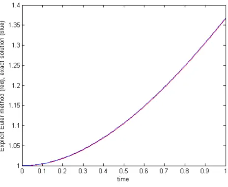
Example 2.1.1. We consider the Cauchy problem

u0 =−u+t+ 1, t∈[0,1],

u(0) = 1. (2.13)

The exact solution is u(t) = exp(−t) +t.

In this problem f(t, u) =−u+t+ 1, therefore

u0(t) = −u(t) +t+ 1,

u00(t) = −u0(t) + 1 =u(t)−t, un000(t) = −u(t) +t,

(17)

i.e., u(0) = 1, u0(0) = 0, u00(0) = 1, u000(0) =−1. The global Taylor method results in the following approximation polynomials:

T1,u(t) = 1,

T2,u(t) = 1 +t2/2,

T3,u(t) = 1 +t2/2−t3/6.

(2.15)

Hence, at the point t = 1 we haveT1,u(1) = 1, T2,u(1) = 1.5, T3,u(1) = 1.333).

(We can also easily define the values T4,u(1) = 1.375 andT5,u(1) = 1.3666.) As

we can see, these values approximate the value of the exact solution u(1) = 1.367879 only for larger values of n.

Let us apply now the local Taylor method taking into account the deriva-tives under (2.14). The algorithm of the first order method is

yi+1 =yi+hi(−yi+ti+ 1), i= 0,1, . . . , N −1, (2.16) while the algorithm of the second order method is

yi+1 =yi+hi(−yi+ti+ 1) + h2_i

2 (yi−ti), i= 0,1, . . . , N −1,

where h1+h2+. . .+hN =T. In our computations we have used the step-size hi = h = 0.1. In Table 2.1 we compared the results of the global and local Taylor methods at the mesh-point of the interval [0,1]. (LT1 and LT2 mean the first and second order local Taylor method, while T1, T2 and T3 are the first, second and third order Taylor methods, respectively.)

Using some numerical method, we can define a numerical solution at the mesh-points of the grid. Comparing the numerical solution with the exact solution, we define the error function, which is a grid function on the mesh on which the numerical method is applied. This error function (which is a vector) can be characterized by the maximum norm. In Table 2.2 we give the magnitude of the maximum norm of the error function on the meshes for decreasing step-sizes. We can observe that by decreasing hthe maximum norm is strictly decreasing for the local Taylor method, while for the global Taylor method the norm does not change. (This is a direct consequence of the fact that the global Taylor method is independent of the mesh-size.)

The local Taylor method is a so-called one-step method (or, alternatively, a two-level method). This means that the approximation at the time level

t = ti+1 is defined with the approximation obtained at the time level t = ti

only. The error analysis is rather complicated. As the above example shows, the difference between the exact solution u(ti+1) and the numerical solution

(18)

ti the exact solution LT1 LT2 T1 T2 T3 0.1 1.0048 1.0000 1.0050 1.0000 1.0050 1.0048 0.2 1.0187 1.0100 1.0190 1.0000 1.0200 1.0187 0.3 1.0408 1.0290 1.0412 1.0000 1.0450 1.0405 0.4 1.0703 1.0561 1.0708 1.0000 1.0800 1.0693 0.5 1.1065 1.0905 1.1071 1.0000 1.1250 1.1042 0.6 1.1488 1.1314 1.1494 1.0000 1.1800 1.1440 0.7 1.1966 1.1783 1.1972 1.0000 1.2450 1.1878 0.8 1.2493 1.2305 1.2500 1.0000 1.3200 1.2347 0.9 1.3066 1.2874 1.3072 1.0000 1.4050 1.2835 1.0 1.3679 1.3487 1.3685 1.0000 1.5000 1.3333

Table 2.1: Comparison of the local and global Taylor methods on the mesh with mesh-size h= 0.1. mesh-size LT1 LT2 T1 T2 T3 0.1 1.92e−02 6.62e−04 0.3679 0.1321 0.0345 0.01 1.80e−03 6.12e−06 0.3679 0.1321 0.0345 0.001 1.85e−04 6.14e−08 0.3679 0.1321 0.0345 0.0001 1.84e−05 6.13e−10 0.3679 0.1321 0.0345

Table 2.2: Maximum norm errors for the local and global Taylor methods for decreasing mesh-size h.

(19)

• The first reason is the local truncation error, which is due to the replace-ment of the Taylor series by the Taylor polynomial, assuming that we know the exact value at the point t = ti. The order of the difference

on the interval [ti, ti+hi], i.e., the order of magnitude of the expression u(t)−Tn,u(t) defines the order of the local error. When this expression

has the order O(hp+1_i ), then the method is called p-th order.

• In each step (except for the first step) of the construction, instead of the exact values their approximations are included. The effect of this inaccuracy may be very significant and they can extremely accumulate during the computation (this is the so-called instability).

• In the computational process we have also round-off error, also called

rounding error, which is the difference between the calculated approxi-mation of a number and its exact mathematical value. Numerical analysis specifically tries to estimate this error when using approximation equa-tions and/or algorithms, especially when using finitely many digits to represent real numbers (which in theory have infinitely many digits). In our work we did not consider the round-off error, which is always present in computer calculations.5

• When we solve our problem on the interval [0, t?_{], then we consider the}

difference between the exact solution and the numerical solution at the point t?_{. We analyze the error which arises due to the first two sources,}

and it is called global error. Intuitively, we say that some method is convergent at some fixed pointt =t? when by approaching zero with the maximum step-size of the mesh the global error at this point tends to zero. The order of the convergence of this limit to zero is called order of convergence of the method. This order is independent of the round-off error. In the numerical computations, to define the approximation at the point t =t?_{, we have to execute approximately} _n _{steps, where} _nh₌ _t?_.

Therefore, in case of local truncation error of the order O(hp+1), the expected magnitude of the global error isO(hp_{). In Table 2.2 the results}

for the methods LT1 and LT2 confirm this conjecture: method LT1 is convergent in the first order, while method LT2 in the second order at the point t? _{= 1.}

The nature of the Taylor method for the differential equation u0 = 1−t√3 _u_can be observed on the link

5_{At the present time there is no universally accepted method to analyze the round-off}

error after a large number of time steps. The three main methods for analyzing round-off accumulation are the analytical method, the probabilistic method and the interval arithmetic method, each of which has both advantages and disadvantages.

(20)

http://math.fullerton.edu/mathews/a2001/Animations/OrdinaryDE/Taylor/ Taylor.html

2.2 Some simple one-step methods

In the previous section we saw that the local Taylor method, especially for

p = 1 is beneficial: for the computation by the formula (2.11) the knowledge of the partial derivatives of the function f is not necessary, and by decreasing the step-size of the mesh the unknown exact solution is well approximated at the mesh-points. Our aim is to define further one-step methods having similar good properties.

The LT1 method was obtained by the approximation of the solution on the subinterval [ti, ti+1] by its first order Taylor polynomial.6 Then the error (the

local truncation error) is

|u(ti+1)−T1,u(ti+1)|=O(h2_i), i= 0,1, . . . , N −1, (2.17) which means that the approximation is exact in the second order. Let us define instead of T1,u(t) some other, first order polynomialP1(t), for which the

estimate (2.17) remains true, i.e., the estimation

|u(ti+1)−P1(ti+1)|=O(h2i) (2.18)

holds.

The polynomial T1,u(t) is the tangent line at the point (ti, u(ti)) to the exact

solution. Therefore, we seek such a first order polynomial P1(t), which passes

through this point, but whose direction is defined by the tangent lines to the solution u(t) at the points ti and ti+1. To this aim, let P1(t) have the form P1(t) := u(ti) +α(t−ti) (t ∈ [ti, ti+1]), where α = α(u0(ti), u0(ti+1)). (E.g.,

by the choice α=u0(ti) we getP1(t) =T1,u(t), and then the estimation (2.18)

holds.)

Is any other suitable choice of α possible? Since

u(ti+1) =u(ti) +u0(ti)hi+O(h2i), (2.19)

therefore

u(ti+1)−P1(ti+1) = hi(u0(ti)−α) +O(h2_i),

i.e., the relation (2.18) is satisfied if and only if the estimation

α−u0(ti) = O(hi) (2.20)

holds.

6_{In each subinterval [}_t

i, ti+1] we define a different Taylor polynomial of the first order,

(21)

Theorem 2.2.1. For any θ ∈_R, under the choice of α by

α= (1−θ)u0(ti) +θu0(ti+1) (2.21)

the estimation (2.20) is true.

Proof. Let us apply (2.19) to the function u0(t). Then we have

u0(ti+1) =u0(ti) +u00(ti)hi+O(h2i). (2.22)

Substituting the relation (2.22) into the formula (2.21), we get

α−u0(ti) =θu00(ti)hi+O(h2_i), (2.23) which proves the statement.

Corollary 2.2.2. The above polynomialP1(t) defines the one-step numerical

method of the form

yi+1 =yi+αhi, (2.24)

where, based on the relations (2.21) and (2.1), we have

α = (1−θ)f(ti, yi) +θf(ti+1, yi+1). (2.25)

Definition 2.2.3. The numerical method defined by (2.24)-(2.25) is called θ -method.

Remark 2.2.1. As for any numerical method, for the θ-method we also as-sume that yi is an approximation to the exact value u(ti), and the difference

between the approximation and the exact value originates – as for the Taylor method – from two sources

a) at each step we replace the exact solution functionu(t) by the first order polynomial P1(t),

b) in the polynomial P1(t) the coefficient α(i.e., the derivatives of the

solu-tion funcsolu-tion) can be defined only approximately.

Since the direction α is defined by the derivatives of the solution at the points

ti and ti+1, therefore we select its value to be between these two values. This

requirement implies that the parameter θ is chosen from the interval [0,1]. In the sequel, we consider three special values of θ ∈[0,1] in more detail.

(22)

2.2.1 Explicit Euler method

Let us consider the θ-method with the choice θ= 0. Then the formulas (2.24) and (2.25) result in the following method:

yi+1 =yi+hif(ti, yi), i= 0,1, . . . , N −1. (2.26)

Since yi is the approximation of the unknown solution u(t) at the point t=ti,

therefore

y0 =u(0) =u0, (2.27)

i.e., in the iteration (2.26) the starting value y0, corresponding to i = 0, is

given.

Definition 2.2.4. The one-step method (2.26)–(2.27) is called explicit Euler method.7 (Alternatively, it is also called forward Euler method.)

In case θ = 0 we have α = u0(ti), therefore the polynomial P1 (which defines

the method) coincides with the first order Taylor polynomial. Therefore the explicit Euler method is the same as the local Taylor method of the first order, defined in (2.11).

Remark 2.2.2. The method (2.26)–(2.27) is called explicit, because the ap-proximation at the point ti+1 is defined directly from the approximation, given

at the point ti.

We can characterize the explicit Euler method (2.26)–(2.27) on the following example, which gives a good insight of the method.

Example 2.2.5. The simplest initial value problem is

u0 =u, u(0) = 1, (2.28)

whose solution is, of course, the exponential function u(t) =et_.

7_{Leonhard Euler (1707–1783) was a pioneering Swiss mathematician and physicist. He}

made important discoveries in fields as diverse as infinitesimal calculus and graph theory. He introduced much of the modern mathematical terminology and notation, particularly for mathematical analysis, such as the notion of a mathematical function. He is also renowned for his work in mechanics, fluid dynamics, optics, and astronomy. Euler spent most of his adult life in St. Petersburg, Russia, and in Berlin, Prussia. He is considered to be the preeminent mathematician of the 18th century, and one of the greatest of all time. He is also one of the most prolific mathematicians ever; his collected works fill between 60 and 80 quarto volumes. A statement attributed to Pierre-Simon Laplace expresses Euler’s influence on mathematics: ”Read Euler, read Euler, he is the master of us all.”

(23)

Since for this problem f(t, u) =u, the explicit Euler method with a fixed step size h >0 takes the form

yi+1 =yi+hyi = (1 +h)yi.

This is a linear iterative equation, and hence it is easy to get

yi = (1 +h)iu0 = (1 +h)i.

Then this is the proposed approximation to the solutionu(ti) = eti _{at the mesh}

point ti =ih. Therefore, when using the Euler scheme to solve the differential

equation, we are effectively approximating the exponential by a power function

eti ₌_eih _≈_{(1 +}_h₎i_.

When we use simply t? _{to indicate the fixed mesh-point} _t

i =ih, we recover, in

the limit, a well-known calculus formula:

et? = lim h→0(1 +h) t?_/h = lim i→∞(1 +t ?_/h₎i_.

A reader familiar with the computation of compound interest will recognize this particular approximation. As the time interval of compounding,h, gets smaller and smaller, the amount in the savings account approaches an exponential.

In Remark 2.2.1 we listed the sources of the error of a numerical method. A basic question is the following: by refining the mesh what is the behavior of the numerical solution at some fixed point t? ∈ [0, T]? More precisely, we wonder whether by increasing the step-size of the mesh to zero the difference of the numerical solution and the exact solution tends to zero. In the sequel, we consider this question for the explicit Euler method. (As before, we assume that the function f satisfies a Lipschitz condition in its second variable, and the solution is sufficiently smooth.)

First we analyze the question on a sequence of refined uniform meshes. Let

ωh :={ti =ih; i= 0,1, . . . , N; h=T /N}

(h→0) be given meshes and assume thatt? _∈_[0_{, T}_{] is such a fixed point which}

belongs to each mesh. Let n denote on a fixed mesh ωh the index for which nh =t?. (Clearly, n depends on h, and in case h →0 the value of n tends to infinity.) We introduce the notation

(24)

for the global error at some mesh-point ti. In the sequel we analyze en by

decreasingh, i.e., we analyze the difference between the exact and the numerical solution at the fixed pointt? forh→0.8 From the definition of the global error (2.29) obviously we have yi =ei +u(ti). Substituting this expression into the

formula of the explicit Euler method of the form (2.26), we get the relation

ei+1−ei =−(u(ti+1)−u(ti)) +hf(ti, ei+u(ti))

= [hf(ti, u(ti))−(u(ti+1)−u(ti))]

+h[f(ti, ei+u(ti))−f(ti, u(ti))].

(2.30)

Let us introduce the notations

gi =hf(ti, u(ti))−(u(ti+1)−u(ti)), ψi =f(ti, ei+u(ti))−f(ti, u(ti)).

(2.31) Hence we get the relation

ei+1−ei =gi+hψi, (2.32)

which is called error equation of the explicit Euler method.

Remark 2.2.3. Let us briefly analyze the two expressions in the notations (2.31). The expression gi shows how exactly the solution of the differential equation satisfies the formula of the explicit Euler method (2.26), written in the formhf(ti, yi)−(yi+1−yi) = 0. This term is present due to the replacement

of the solution function u(t) on the interval [ti, ti+1] by the first order Taylor polynomial. The second expressionψi characterizes the magnitude of the error,

arising in the formula of the method for the computationyi+1, when we replace

the exact (and unknown) value u(ti) by its approximationyi. Due to the Lipschitz property, we have

|ψi|=|f(ti, ei+u(ti))−f(ti, u(ti))| ≤L|(ei+u(ti))−u(ti)|=L|ei|. (2.33)

Hence, based on (2.32) and (2.33), we get

|ei+1| ≤ |ei|+|gi|+h|ψi| ≤(1 +hL)|ei|+|gi| (2.34)

8_{Intuitively it is clear that the condition} _t? _∈ _ω

h for any h > 0 can be relaxed: it is

enough to assume that the sequence of mesh-points (tn) is convergent to the fixed pointt?,

(25)

for any i = 0,1, . . . , n−1. Using this relation, we can write the following estimation for the global error en:

|en| ≤(1 +hL)|en−1|+|gn−1| ≤(1 +hL) [(1 +hL)|en−2|+|gn−2|] +|gn−1| = (1 +hL)2|en−2|+ [(1 +hL)|gn−2|+|gn−1|]≤. . . ≤(1 +hL)n|e0|+ n−1 X i=0 (1 +hL)i|gn−1−i| <(1 +hL)n " |e0|+ n−1 X i=0 |gn−1−i| # . (2.35) (In the last step we used the obvious estimation (1 +hL)i _< _{(1 +}_hL₎n_, _i ₌

0,1, . . . , n− 1.) Since for any x > 0 the inequality 1 +x < exp(x) holds, therefore, by use of the equality nh = t?, we have(1 +hL)n < exp(nhL) = exp(Lt?_{). Hence, based on (2.35), we get}

|en| ≤exp(Lt?) " |e0|+ n−1 X i=0 |gn−1−i| # . (2.36)

Let us give an estimation for |gi|. One can easily see that the equality

u(ti+1)−u(ti) = u(ti+h)−u(ti) =hu0(ti) +

1 2u

00

(ξi)h2 (2.37)

is true, where ξi ∈ (ti, ti+1) is some fixed point. Since f(ti, u(ti)) = u0(ti),

therefore, according to the definition of gi in (2.31), the inequality |gi| ≤ M2 2 h 2_, _M 2 = max [0,t?_]|u 00 (t)| (2.38)

holds. Using the estimations (2.36) and (2.38), we get

|en| ≤exp(Lt?) |e0|+hnM2 2 h = exp(Lt?) |e0|+ t ?_M2 2 h . (2.39) Since e0 = 0, therefore, |en| ≤exp(Lt?) t?M2 2 h. (2.40)

Hence, in case h→0 we have en →0, moreover, en=O(h).

The convergence of the explicit Euler method on some suitably chosen, non-uniform mesh can be shown, too. Further we will show it. Let us consider the sequence of refined meshes

(26)

We use the notations hi = ti+1 −ti, i = 0,1, . . . , N − 1 and h = T /N. In

the sequel we assume that with increasing the number of mesh-points the grid becomes finer everywhere, i.e., there exists a constant 0< c <∞ such that

hi ≤ch, i= 1,2, . . . , N (2.41)

for any N. We assume again that the fixed point t? _∈ _[0_{, T}_{] is an element}

of each mesh. As before, on some fixed mesh n denotes the index for which

h0+h1 +. . .+hn−1 =t?.

Using the notations

gi =hif(ti, u(ti))−(u(ti+1)−u(ti)), ψi =f(ti, ei +u(ti))−f(ti, u(ti))

(2.42) the estimation (2.34) can be rewritten as follows:

|ei+1| ≤ |ei|+|gi|+hi|ψi| ≤ |ei|+|gi|+hiL|ei| ≤

(1 +hiL)|ei|+|gi| ≤exp(hiL)|ei|+|gi| ≤exp(hiL) [|ei|+|gi|].

(2.43)

Then the estimation (2.35), taking into account (2.43), results in the relation

|en| ≤exp(hn−1L) [|en−1|+|gn−1|] ≤exp(hn−1L) [exp(hn−2L) (|en−2|+|gn−2|) +|gn−1|] = exp((hn−1+hn−2)L) (|en−2|+|gn−2|+gn−1|) ≤exp((hn−1+hn−2+. . .+h0)L) " |e0|+ n X i=1 |gn−i| # . (2.44)

Due to the relation hn−1+hn−2+. . .+h0 =t? and the estimation

|gi| ≤ M2 2 h 2 i ≤ M2c2 2 h 2_, _(2.45)

the relations (2.44) and (2.45) together imply the estimation

|en| ≤exp(t?L) |e0|+hn M2c2 2 h = exp(t?L) |e0|+t? M2c2 2 h . (2.46)

The estimation (2.46) shows that on a sequence of suitably refined meshes by

h →0 we have en→0, and moreover, en =O(h).

(27)

Theorem 2.2.6. The explicit Euler method is convergent, and the rate of con-vergence is one.9

Remark 2.2.4. We can see that for the explicit Euler method the choicey0 = u0 is not necessary to obtain the convergence, i.e., the relation limh→0en = 0.

Obviously, it is enough to require only the relation y0 = u0 +O(h), since in

this case e0 = O(h). (By this choice the rate of the convergence en = O(h)

still remains true.)

2.2.2 Implicit Euler method

Let us consider the θ-method by the choice θ = 1. For this case the formulas (2.24) and (2.25) together generate the following numerical method:

yi+1 =yi+hif(ti+1, yi+1), i= 0,1, . . . , N −1, (2.47)

where again we put y0 =u0.

Definition 2.2.7. The one-step numerical method defined under (2.47)is called

implicit Euler method.

Remark 2.2.5. The Euler method of the form (2.47) is called implicit because

yi+1, the value of the approximation on the new time levelti+1, can be obtained

by solving a usually non-linear equation. E.g., for the function f(t, u) = sinu, the algorithm of the implicit Euler method reads as yi+1 =yi+hisinyi+1, and

hence the computation of the unknown yi+1 requires the solution of a

non-linear algebraic equation. However, when we set f(t, u) = u, then we have the algorithmyi+1 =yi+hiyi+1, and from this relationyi+1can be defined directly,

without solving any non-linear equation.

For the error functionei of the implicit Euler method we have the following

equation:

ei+1−ei =−(u(ti+1)−u(ti)) +hif(ti+1, u(ti+1) +ei+1)

= [hif(ti+1, u(ti+1))−(u(ti+1)−u(ti))]

+hi[f(ti+1, u(ti+1) +ei+1)−f(ti+1, u(ti+1))].

(2.48)

Hence, by the notations

gi =hif(ti+1, u(ti+1))−(u(ti+1)−u(ti)), ψi =f(ti+1, u(ti+1) +ei+1)−f(ti+1, u(ti+1))

(2.49)

9_{We remind that the order of the convergence is defined by the order of the global error,}

(28)

we arrive again at the error equation of the form (2.32). Clearly, we have

u(ti+1)−u(ti) =u(ti+1)−u(ti+1−h) =hiu0(ti+1)−

1 2u

00

(ξi)h2i, (2.50)

where ξi ∈ (ti, ti+1) is some given point. On the other side, f(ti+1, u(ti+1)) = u0(ti+1). Hence for gi, defined in (2.49), we have the inequality

|gi| ≤ M2

2 h

2

i. (2.51)

However, for the implicit Euler method the value of ψi depends both on the

approximation and on the exact solution at the point ti+1, therefore, the proof

of the convergence is more complicated than it was done for the explicit Euler method. In the following we give an elementary proof on a uniform mesh, i.e., for the case hi =h.

We consider the implicit Euler method, which means that the values yi at

the mesh-points ωh are defined by the one-step recursion (2.47). Using the

Lipschitz property of the function f, from the error equation (2.32) we obtain

|ei+1| ≤ |ei|+hL|ei+1|+|gi|, (2.52) which implies the relation

(1−Lh)|ei+1| ≤ |ei|+|gi|. (2.53)

Assume that h < h0 :=

1

2L. Then (2.53) implies the relation |ei+1| ≤

1

1−hL|ei|+

1

1−hL|gi|. (2.54)

We give an estimation for 1

1−hL. Based on the assumption,hL ≤0.5,

there-fore we can write this expression as 1< 1 1−hL = 1 +hL+ (hL) 2 ₊_{· · ·}_{+ (}_hL₎n₊_{· · ·}₌ 1 +hL+ (hL)2 1 +hL+ (hL)2+. . .= 1 +hL+ (hL)2 1 1−hL. (2.55)

Obviously, for the values Lh <0.5 the estimation (hL)

2

1−hL < hL holds.

There-fore, we have the upper bound 1

(29)

Since for the values Lh∈[0,0.5] we have 1

1−hL ≤2, therefore for the global

error the substitution (2.56) into (2.54) results in the recursive relation

|ei| ≤exp(2hL)|ei−1|+ 2|gi|. (2.57)

Due to the error estimation (2.51), we have

|gi| ≤ M2

2 h

2 _:=_g

max for all i= 1,2, . . . , N. (2.58)

Therefore, based on (2.57), we have the recursion

|ei| ≤exp(2hL)|ei−1|+ 2gmax. (2.59)

The following statement is simple, and its proof by induction is left for the Reader.

Lemma 2.2.8. Leta >0andb ≥0given numbers, andsi (i= 0,1, . . . , k−1)

such numbers that the inequalities

|si| ≤a|si−1|+b, i= 1, . . . , k−1 (2.60)

hold. Then the estimations

|si| ≤ai|s0|+ ai₋₁

a−1b, i= 1,2, . . . , k (2.61)

are valid.

Hence, we have

Corollary 2.2.9. When a >1, then obviously

ai−1

a−1 =a

i−1 ₊_ai−2₊_{· · ·}_{+ 1} _≤_iai−1_.

Hence, for this case Lemma 2.2.8, instead of (2.61) yields the estimation

|si| ≤ai|s0|+iai−1b, i= 1,2, . . . , k. (2.62)

Let us apply Lemma 2.2.8 to the global errorei. Choosinga = exp(2hL)>

1, b = 2gmax ≥ 0, and taking into account the relation (2.59), based on (2.62)

we get

|ei| ≤[exp(2hL)]i|e0|+i[exp(2hL)]i

−1

(30)

Due to the obvious relations

[exp(2hL)]i = exp(2Lhi) = exp(2Lti),

and

i[exp(2hL)]i−12gmax <2ihexp(2Lhi)gmax

h = 2tiexp(2Lti) gmax

h ,

the relation (2.63) results in the estimation

|ei| ≤exp(2Lti) h |e0|+ 2ti gmax h i , (2.64)

which holds for every i= 1,2, . . . , N.

Using the expression for gmax in (2.58), from the formula (2.63) we get

|ei| ≤exp(2Lti) [|e0|+M2hti], (2.65)

for any i= 1,2, . . . , N.

Let us apply the estimate (2.65) for the index n. (Remember that on a fixed meshωh, ndenotes the index for which nh=t?, where t? ∈[0, T] is some

fixed point, where the convergence is analyzed.) Then we get

|en| ≤exp(2Ltn) [|e0|+M2htn] = exp(2Lt?) [|e0|+M2ht?]. (2.66)

Since e0 = 0, therefore, finally we get

|en| ≤C·h, (2.67)

where C =M2t?exp(2Lt?) =constant. This proves the following statement.

Theorem 2.2.10. The implicit Euler method is convergent, and the rate of convergence is one.

Finally, we make two comments.

• The convergence on the interval [0, t?] yields the relation lim

h→0i=1,2,...,nmax |ei|= 0.

As one can easily see, the relation |en| ≤ C ·h holds for both methods

(explicit Euler method and implicit Euler method). Therefore the lo-cal truncation error |en| can be bounded at any point uniformly on the

interval [0, t?_{], which means first order convergence on the interval.} • Since the implicit Euler method is implicit, in each step we must solve

a – usually non-linear – equation, namely, find the root of the equation

g(s) :=s−hf(tn, s)−yn = 0. This can be done by using some iterative

(31)

2.2.3 Trapezoidal method

Let us consider the θ-method by the choiceθ = 0.5. For this case the formulas (2.24) and (2.25) generate the numerical method of the form

yi+1−yi = hi

2 [f(ti, yi) +f(ti+1, yi+1)], i= 0,1, . . . , N −1, (2.68) where y0 =u0.

Definition 2.2.11. The one-step method (2.68) is called trapezoidal method.

We remark that the trapezoidal method is a combination of the explicit Euler method and the implicit Euler method. Clearly, this method is implicit, like the implicit Euler method. We also note that this method is sometimes also called Crank–Nicolson method, due to the application of this method to the numerical solution of the semi-discretized heat conduction equation.

By combining the error equation for the explicit Euler method and the im-plicit Euler method, we can easily obtain the error equation for the trapezoidal method in the form (2.32) again. One can easily verify that for this method we get

gi =

1

2hi[f(ti, u(ti)) +f(ti+1, u(ti+1))]−(u(ti+1)−u(ti)),

ψi =

1

2[f(ti, u(ti) +ei)−f(ti, u(ti))] + 1

2[f(ti+1, u(ti+1) +ei+1)−f(ti+1, u(ti+1))].

(2.69)

Let us estimate gi in (2.69). Using the notation ti+1₂ = ti + 0.5hi we develop u(t) around this point into the Taylor series with the Lagrange remainder:

u(ti) =u(ti+1₂ −hi/2) and u(ti+1) = u(ti+1₂ +hi/2). Then

u(ti+1)−u(ti) = hiu0(ti+1/2) + h3 i 48(u 000 (ξ_i1) +u000(ξ_i2)), (2.70) where ξ1

i, ξi2 ∈(ti, ti+1) are given points. On the other hand, we have

f(ti, u(ti)) +f(ti+1, u(ti+1)) =u0(ti) +u0(ti+1). (2.71) Developing again the functions on the right side of (2.71) around the point

t =t_i+1

2, we get the equality 1 2[f(ti, u(ti)) +f(ti+1, u(ti+1))] =u 0 (t_i+1 2) + h2_i 16(u 000 (ξ_i3) +u000(ξ_i4)). (2.72)

(32)

ti exact solution EE IE TR 0.1 1.0048 1.0000 1.0091 1.0048 0.2 1.0187 1.0100 1.0264 1.0186 0.3 1.0408 1.0290 1.0513 1.0406 0.4 1.0703 1.0561 1.0830 1.0701 0.5 1.1065 1.0905 1.1209 1.1063 0.6 1.1488 1.1314 1.1645 1.1485 0.7 1.1966 1.1783 1.2132 1.1963 0.8 1.2493 1.2305 1.2665 1.2490 0.9 1.3066 1.2874 1.3241 1.3063 1.0 1.3679 1.3487 1.3855 1.3676

Table 2.3: Comparison in the maximum norm for the explicit Euler method (EE), the implicit Euler method (IE), and the trapezoidal method (TR) on the mesh with mesh-size h= 0.1.

Hence, using the relations (2.70) and (2.72), for the local approximation error

gi we get |gi| ≤ M3 6 h 3 i, M3 = max [0,t?_]|u 000 (t)|. (2.73)

We consider the test equation given in Exercise 2.13. In Table (2.3) we give the numerical solution by the above listed three numerical methods (explicit Euler method, implicit Euler method, trapezoidal method). In Table (2.4) we compare the numerical results obtained on refining meshes in the maximum norm. These results show that on some fixed mesh the explicit Euler method and the implicit Euler method give approximately the same accuracy, while the trapezoidal method is more accurate. On the refining meshes we can observe that the error function of the trapezoidal method has the order O(h2_{), while}

for the explicit Euler method and the implicit Euler method the error function is of O(h). (These results completely correspond to the theory.)

2.2.4 Alternative introduction of the one-step methods

The discussed one-step numerical methods can be introduced in other ways, too. One possibility is the following. Let u(t) be the solution of the Cauchy problem (1.6), which means that the identity (2.3) holds on the interval [0, T]. Integrating both sides of this identity between two neighboring mesh-points of

(33)

step-size (h) EE IE TR 0.1 1.92e−02 1.92e−02 3.06e−04 0.01 1.84e−03 1.84e−03 3.06e−06 0.001 1.84e−04 1.84e−04 3.06e−08 0.0001 1.84e−05 1.84e−05 3.06e−10 0.0001 1.84e−06 1.84e−06 5.54e−12

Table 2.4: The error in the maximum norm for the explicit Euler method (EE), the implicit Euler method (IE), and the trapezoidal method (TR) on the mesh with mesh-size h.

the mesh ωh, we get

u(ti+1)−u(ti) =

Z ti+1

ti

f(t, u(t))dt, t∈[0, T] (2.74) for any i= 0,1, . . . , N −1. To define some numerical method, on the interval [ti, ti+1] we integrate numerically the right side of this relation. The simplest integration formulas are using the end-points of the interval, only. The different integration formulas result in the above methods.

• The simplest way is using the value taken on the left-hand side of the interval, i.e., the integration rule

Z ti+1

ti

f(t, u(t))dt ≈hif(ti, u(ti)). (2.75) Then (2.74) and (2.75) together result in the formula (2.26), which is the explicit Euler method.

• Another possibility is using the value taken on the right-hand side of the interval, i.e., the integration rule

Z ti+1

ti

f(t, u(t))dt ≈hif(ti+1, u(ti+1)). (2.76)

Then (2.74) and (2.76) result in the formula (2.47), which is the implicit Euler method.

• When we use the trapezoidal rule for the numerical integration in (2.74), i.e., the formula

Z ti+1

ti

f(t, u(t))dt≈ hi

(34)

is applied, then (2.74) and (2.77) together result in the formula (2.68), i.e., the trapezoidal method.

• Using the numerical integration formula

Z ti+1

ti

f(t, u(t))dt≈hi[(1−θ)f(ti, u(ti)) +θf(ti+1, u(ti+1))], (2.78)

we obtain the θ-method, which was already defined by formulas (2.24)-(2.25).

In order to re-obtain the numerical formulas, another approach is the fol-lowing. We consider the identity (2.3) at some fixed mesh-point, and for the left side we use some numerical derivation rule.

• When we use the point t = ti, and we write the identity (2.3) at this

point, then we get u0(ti) = f(ti, u(ti)). Let us apply the forward finite

difference approximation to the derivative on the left-hand side, then we get the approximation u0(ti)' (u(ti+1)−u(ti))/hi. These two formulas

together generate the explicit Euler method.

• When we write the identity (2.3) at the point t = ti+1, and we use the retrograde numerical finite difference derivation, then we obtain the implicit Euler method.

• The arithmetic mean of the above formulas result in the trapezoidal method.

The behavior of the above methods for the equation u0 = 1−t√3_u _{can be} seen on the animation under the link

http://math.fullerton.edu/mathews/a2001/Animations/Animations9.html

2.3 The basic concepts of general one-step

meth-ods

In this section on the uniform mesh

ωh :={ti =ih; i= 0,1, . . . , n; h=T /N}

(or on their sequence) we formulate the general form of one-steps methods, and we define some basic concepts of such methods. We consider the numerical method of the form

(35)

where Φ is some given function. In the sequel, the numerical method, defined by (2.79) is called Φ numerical method (in short, Φ-method).

Remark 2.3.1. By some special choice of the function Φ the previously dis-cussed one-step methods can be written in the form (2.79). E.g.

• by the choice Φ(h, ti, yi, yi+1) = f(ti, yi) we get the explicit Euler method; • by the choice Φ(h, ti, yi, yi+1) = f(ti+h, yi+1) we get the implicit Euler

method;

• by the choice Φ(h, ti, yi, yi+1) = 0.5 [f(ti, yi) +f(ti+h, yi+1)] we get the

trapezoidal method,

• by the choice Φ(h, ti, yi, yi+1) = (1−θ)f(ti, yi) +θf(ti+h, yi+1) we get

the θ-method.

Definition 2.3.1. The numerical methods withΦ = Φ(h, ti, yi)(i.e., the

func-tion Φ is independent of yi+1) are called explicit methods. When Φ really depends on yi+1, i.e., Φ = Φ(h, ti, yi, yi+1), the numerical method is called

im-plicit.

As before, u(t) denotes the exact solution of the Cauchy problem (2.1)– (2.2), and let t? ∈(0, T] be some given point.

Definition 2.3.2. The functionet?(h) = yn−u(t?),(nh=t?) is called global

discretization error of theΦ numerical method at the point t?. We say that the

Φ numerical method is convergent at the point t?, when the relation

lim

h→0eh(t?) = 0 (2.80)

holds. When the Φnumerical method is convergent at each point of the interval

[0, T], then the numerical method is called convergent method. The order of the convergence to zero in (2.80) is called order of the convergence of the Φ -method.

The local behavior of the Φ-method can be characterized by the value which is obtained after one step using the exact solution as starting value. This value

ˆ

yi+1, being an approximation to the exact solution, is defined as

ˆ

(36)

Definition 2.3.3. The mesh-function li(h) = ˆyi−u(ti) (where ti =ih ∈ ωh)

is called local discretization error of the Φ-method, defined in (2.79), at the point ti.

For the implicit Φ-methods the calculation of the local discretization error is usually difficult, because one has to know the value ˆyi+1 from the formula

(2.81). To avoid this difficulty, we introduce the mesh-function

gi(h) = −u(ti+1) +u(ti) +hΦ(h, ti, u(ti), u(ti+1)). (2.82)

The order of this expression (using the equation in the Cauchy problem) can be defined directly, without knowing the exact solution, by developing into Taylor series.

Definition 2.3.4. The function gi(h) is called local truncation error of the

Φ-method, defined in (2.79), at the point ti. We say that the Φ-method is

consistent of order r, when

gi(h) =O(hr+1) (2.83)

with some constant r >0 for any mesh-point ti ∈ωh.

Obviously, the truncation error and its order shows how exactly the exact solution satisfies the formula of the Φ-method.10

Remark 2.3.2. Based on the estimations (2.38), (2.51) and (2.73) we can see that both the explicit Euler method and the implicit Euler method are consistent of first order, while the trapezoidal method has of second order consistency. An elementary calculation shows that the θ-method is of second order only for θ = 0.5 (which means the trapezoidal method), otherwise it is consistent of first order .

Further we assume that the function Φ in the numerical method (2.79) satisfies the Lipschitz condition w.r.t. its third and fourth variables, which means the following: there exist constants L3 ≥ 0 and L4 ≥ 0 such that for

any numbers s1, s2, p1 and p2 the inequality

|Φ(h, ti, s1, p1)−Φ(h, ti, s2, p2)| ≤L3|s1−s2|+L4|p1−p2| (2.84) holds for all ti ∈ωh and h >0. When the function Φ is independent on yi (or

on yi+1), thenL3 = 0 (or L4 = 0).

Remark 2.3.3. According to the Remark 2.3.1, when the functionf satisfies the Lipshitz condition w.r.t. its second variable, then Φ, corresponding to the

θ-method for any θ satisfies (2.84) with some suitably chosen L3 and L4.

10_{The global discretization error, defined as} _e

t?(h) =yn−u(t?) is also called global

trun-cation error, which is, in fact the accumulation of the local truncation error over all of the iterations, assuming perfect knowledge of the true solution at the initial time step.

(37)

2.3.1 Convergence of the one-step methods

Further we analyze the convergence of the Φ-method, given by (2.84). We assume that it satisfies the Lipschitz condition w.r.t. its second and third variables, and it is consistent of orderr. For the sake of simplicity, we introduce the notations

eti(h) = ei, gi(h) =gi, li(h) = li. (2.85)

According to the definition of the local and global discretization errors, we have the following relations:

ei+1 =yi+1−u(ti+1) = (yi+1−yˆi+1)+(ˆyi+1−u(ti+1)) = (yi+1−yˆi+1)+li (2.86)

Hence,

|ei+1| ≤ |yi+1−yˆi+1|+|li| (2.87)

and we give an overestimate for both expressions on the right side of (2.87). For the local discretization error we have

li+1= ˆyi+1−u(ti+1)

=u(ti) +hΦ(h, ti, u(ti),yˆi+1))−u(ti+1)

=−u(ti+1) +u(ti) +hΦ(h, ti, u(ti), u(ti+1))

+h[Φ(h, ti, u(ti),yˆi+1))−Φ(h, ti, u(ti), u(ti+1))]

=gi+h[Φ(h, ti, u(ti),yi+1ˆ ))−Φ(h, ti, u(ti), u(ti+1))].

(2.88)

Hence, using the condition (2.84), we get

|li+1| ≤ |gi|+hL4|yi+1ˆ −u(ti+1)|=|gi|+hL4|li+1|. (2.89) Therefore, based on (2.89), the estimation

|li+1| ≤

1 1−hL4

|gi| (2.90)

holds.

Remark 2.3.4. The inequality (2.90) shows that the order of the local ap-proximation error cannot be less than the order of the consistency. (I.e., if the method is consistent of orderr, then he local approximation error tends to zero with a rate not less than r.)

(38)

We have

|yi+1−yˆi+1|=

|(yi+hΦ(h, ti, yi, yi+1))−(u(ti) +hΦ(h, ti, u(ti),yi+1ˆ ))| ≤ |ei|+h|Φ(h, ti, yi, yi+1)−Φ(h, ti, u(ti),yˆi+1)|

≤ |ei|+hL3|yi−u(ti)|+hL4|yi+1−yˆi+1|

= (1 +hL3)|ei|+hL4|yi+1−yˆi+1|.

(2.91)

Hence, based on (2.91), the inequality

|yi+1−yi+1| ≤ˆ 1 +hL3 1−hL4

|ei| (2.92)

holds. Using the relations (2.90) and (2.92), the inequality (2.87) can be rewrit-ten as |ei+1| ≤ 1 +hL3 1−hL4 |ei|+ 1 1−hL4 |gi|. (2.93)

Let us introduce the notations

µ=µ(h) = 1 +hL3 1−hL4

, χ=χ(h) = 1 1−hL4

. (2.94)

Remark 2.3.5. With the notations (2.94) we have

µ= 1 +hL3+L4

1−hL4

, (2.95)

therefore µ= 1 +O(h). Consequently, we can choose constants h0, µ0 and λ0

such that the estimations

µ=µ(h)≤1 +µ0h, χ=χ(h)≤χ0, ∀h∈(0, h0) (2.96)

are true11_.

Using the notation (2.94), the estimation (2.93) can be written as

|ei+1| ≤µ|ei|+χ|gi|. (2.97) Applying the relation (2.97) recursively, we obtain the inequality

|en| ≤µ|en−1|+χ|gn−1| ≤µ[µ|en−2|+χ|gn−2|] +χ|gn−1|=µ2|en−2| +χ[µ|gn−2|+|gn−1|]≤. . .≤µn|e0|+χ n−1 X i=0 µi|gn−1−i| ≤µn " |e0|+χ n−1 X i=0 |gn−1−i| # . (2.98) 11_E.g.,_h 0= _2L1₄, µ0= 2(L3+L4) andχ0= 2.

(39)

Using (2.96), for any h∈(0, h0) we have χ≤χ0 and

µn≤(1 +µ0h)n ≤exp(µ0hn) = exp(µ0t?). (2.99)

Therefore, by using (2.98), the estimate

|en| ≤exp(µ0t?) " |e0|+χ0 n−1 X i=0 |gn−1−i| # (2.100)

holds. Since the Φ-method is consistent of orderr, therefore, due to the defini-tion (2.80), for a sufficiently small h we have |gi| ≤c0hr+1 with some constant

c0 ≥0. Hence, for small values of h we get n−1

X

i=0

|gn−1−i| ≤nc0hr+1 =c0t?hr. (2.101)

Comparing the formulas (2.100) and (2.101), we get the estimation

|en| ≤exp(µ0t?) [|e0|+c1hr], (2.102)

where c1 =χ0c0t?=constant.

Since e0 = 0, therefore from (2.102) the following statement is proven.

Theorem 2.3.5. Assume that theΦnumerical method, defined by the formula

(2.79), has the following properties:

• it is consistent of order r;

• for the function Φ the Lipschitz condition (2.84) is satisfied.

Then the Φ-method is convergent on the interval [0, T] and the order of the convergence is r.

Corollary 2.3.6. Using Remark 2.3.2 and Remark 2.3.3, it is clear that the

θ-method for θ = 0.5 is convergent in second order, otherwise its order of convergence is equal to one.

Remark 2.3.6. In this part the convergence was proven from the relation (2.97), namely, using two properties of the terms appearing in this expression:

• the method is consistent, i.e., gi = O(hr+1) with some positive number r, and the function χ(h) is bounded;

(40)

• for the function µ(h) the estimation (2.96) holds. (This property shows that passing from some time level to the next one, with increasing the number of the steps (i.e., with decreasing h) the error remains bounded. This property is called stability of the method.

Hence, Theorem 2.3.5 shows that for well-posed Cauchy problems the consis-tency and stability of the Φ-method guarantees the convergence. (The stability can be guaranteed by the Lipschitz condition for the function f on right side of the differential equation in the Cauchy problem (2.1)-(2.2).)

2.4 Runge–Kutta method

As we have seen, the maximum accuracy of the investigated one-step meth-ods (explicit Euler method, implicit Euler method, trapezoidal method, θ -method) for the Cauchy problem (2.1)-(2.2) is two. However, from a practical point of view, this accuracy is not enough: typically we require the construc-tion of numerical methods with higher order of accuracy. The accuracy of the Taylor method is higher, but, in this case the realization of this method re-quires rather complicated preliminary analysis. (Determination of all partial derivatives and its evaluation at given points.) In this section we show that, by use of some simple idea, the task of determining the partial derivatives can be omitted.

2.4.1 Second order Runge–Kutta methods

Let us consider again the Cauchy problem (2.1)–(2.2). In order to introduce the Runge–Kutta methods, first of all we define a one-step method of second order accuracy, which is different from the trapezoidal method.

Let us define the first terms of the Taylor series of the functionu(t) in the form (2.6) at the point t=t?₊_h_{. Then}

u(t?+h) = u(t?) +hu0(t?) + h

2

2!u 00

(t?) +O(h3). (2.103) Using the derivatives (2.4), and introducing the notations

f =f(t?, u(t?)), ∂if =∂if(t?, u(t?)), ∂ijf =∂ijf(t?, u(t?)), etc.,

the equation (2.103) can be rewritten as

u(t?+h) =u(t?) +hf +h 2 2!(∂1f +f ∂2f) +O(h 3₎ =u(t?) + h 2f+ h 2[f+h∂1f +hf ∂2f] +O(h 3₎_. (2.104)

(41)

Since 12

f(t?+h, u(t?) +hf(t?, u(t?)) =f +h∂1f+hf ∂2f+O(h2), (2.105)

therefore (2.104) can be written in the form

u(t? +h) = u(t?) + h 2f + h 2(f(t ? +h, u(t?) +hf(t?, u(t?))) +O(h3). (2.106) Therefore, applying the formula (2.106) at some arbitrary mesh-point ti = t?

of ωh, we can define the following one-step, explicit numerical method: yi+1 =yi+ h

2f(ti, yi) +

h

2f(ti+1, yi+hf(ti, yi)). (2.107) Let us introduce the notations

k1 =f(ti, yi); k2 =f(ti+1, yi+hf(ti, yi)) = f(ti +h, yi+hk1). (2.108)

Then the method (2.107) can be written in the form

yi+1 =yi+h

2(k1+k2). (2.109)

Definition 2.4.1. The one-step, explicit numerical method (2.108)-(2.109) is called Heun method13_.

Remark 2.4.1. Based on (2.106), we have

u(t?+h)−u(t?)−h

2f −

h

2(f(t

?₊_{h, u}₍_t?_{) +}_hf₍_t?_{, u}₍_t?_{))) =}_O₍_h3₎_. _(2.110)

This means that the exact solution of the Cauchy problem (2.1)-(2.2) satisfies the formula of the Heun method (2.107) with the accuracyO(h3_{), which means}

that the Heun method is of second order.

Some further details of the Heun method can be found under the link

http://math.fullerton.edu/mathews/n2003/Heun’sMethodMod.html

Here one can also see an animation for the behavior of the numerical solution, obtained by the Heun method, for the differential equation u0 = 1−t√3_u_.

12_{We recall that the first order Taylor polynomial of the function} _f _: _Q

T → R around

the point (t, u) , for arbitrary constantsc1, c2 ∈Rcan be written as f(t+c1h, u+c2h) =

f(t, u) +c1h∂1f(t, u) +c2h∂2f(t, u) +O(h2).

13_{The method is named after Karl L. W. M. Heun (1859–1929), who was a German}