R E P O R T
Evaluation of an online learning approach
for robust object tracking
Georg Nebehay Branislav Micusik Cristina Picus Roman Pflugfelder
Evaluation of an online learning approach for
robust object tracking
G. Nebehay; B. Micusik, C. Picus, R. Pflugfelder AIT Austrian Institute of Technology
{georg.nebehay.fl, branislav.micusik, cristina.picus, roman.pflugfelder} @ait.ac.at
TR AIT-DSS-0279
Abstract
Current state-of-the-art methods for object tracking perform adaptive tracking-by-detection, meaning that a detector predicts the position of an object and adapts its parameters to the object’s appearance at the same time. While suit-able for cases when the object does not disappear from the scene, these meth-ods tend to fail on occlusions. In this work, we build on a novel approach called Tracking-Learning-Detection (TLD) that overcomes this problem. In methods based on TLD, a detector is trained with examples found on the trajectory of a tracker that itself does not depend on the object detector. By decoupling object tracking and object detection we achieve high robustness and outperform existing adaptive tracking-by-detection methods. We show that by using simple features for object detection and by employing a cas-caded approach a considerable reduction of computing time is achieved. We evaluate our approach both on existing standard single-camera datasets as well as on newly recorded sequences in multi-camera scenarios.
1
Introduction
The visual cortex of the human brain locates and identifies objects by analysing the information arriving as action potentials that are triggered in the retina [20]. While perceptual psychologists study how the human visual system interprets environ-mental stimuli, researchers incomputer visiondevelop mathematical techniques in order to extract information about physical objects based on camera images [44]. Computer vision methods are applied to optical character recognition, quality in-spection, robot guidance, scene reconstruction and object categorisation [47]. One domain of research in computer vision isobject tracking, in which methods are studied that estimate the location of targets in consecutive video frames [34]. The proliferation of high-powered computers, the availability of high quality and inex-pensive video cameras, and the need for automated video analysis have drawn in-terest to applying object tracking algorithms in automated surveillance, automatic
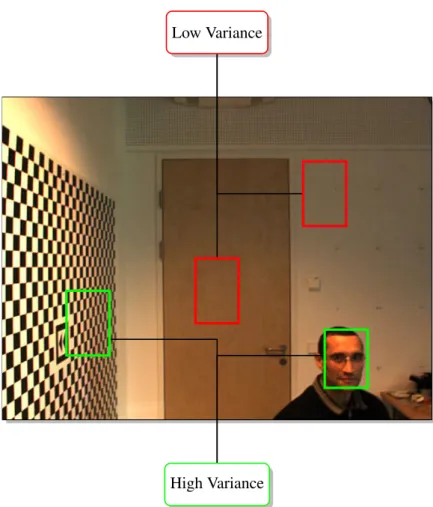
Figure 1: The state of an object encoded in a bounding box. The enlarged patch constrained by the bounding box is displayed on the right. The image is part of the PETS 20091dataset.
annotation of video data, human-computer interaction, traffic monitoring and ve-hicle navigation [50].
1.1 Problem Definition
In this work we focus on semi-automated single-target tracking. The problem of
single-target tracking is defined as follows [34]. Given a sequence of images I1. . .In, estimate the statexkof the target for each frameIk. Object tracking meth-ods encode the statexkas centroids, bounding boxes, bounding ellipses, chains of points or shape [34]. For example, in Fig.1, a bounding box is shown around an object of interest. In this case, the parameters ofxkconsist of the upper left corner of the rectangle(x,y)and its width and height. Maggio and Cavallaro [34] group approaches based on the amount of user interaction that is required to identify the objects of interest.Manual trackingrequires the interaction with the user in every frame. Automated trackingmethods use a priori information in order to initialise the tracking process automatically. Insemi-automatedtracking, user input is re-quired in order to initialise the tracking process.
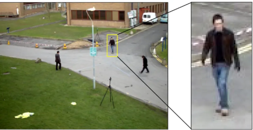
According to Maggio and Cavallaro [34], the main challenge in object tracking isclutter. Clutter is the phenomenon when features expected from the object of interest are difficult to discriminate against features extracted from other objects in the scene. In Fig.2an example for clutter is shown. In this image, several objects are present that are similar in shape to the object of interest. Another challenge is introduced byappearance variationsof the target itself. Intrinsic appearance vari-ability include pose variation and shape deformation, whereas extrinsic appearance variability include illumination change, camera motion and different camera view-points [41]. Approaches that maintain a template of the object of interest typically face thetemplate update problemthat relates to the question of how to update an existing template so that it remains a representative model [35]. If the original
tem-Figure 2: The main challenge in object tracking is to the distinguish the object of interest (green) from clutter in the background (red). Image is from [10].
plate is never changed, it will eventually no longer be an accurate representation of the model. When the template is adapted to every change in appearance, errors will accumulate and the template will steadilydriftaway from the object. This problem is closely related to thestability-plasticity dilemma, which relates to the trade-off between the stability required to retain information and the plasticity re-quired for new learning [22]. This dilemma is faced by all learning systems [1]. Objects undergoocclusionswhen covered by other object or when they leave the field of view of the camera. In order to handle such cases, a mechanism is neces-sary that re-detects the object independently of its last position in the image [50]. Requirements on theexecution timepose another difficulty. [50].
1.2 Related Work
Lepetit et al. [30] identify two paradigms in object tracking. Recursive tracking
methods estimate the current state xt of an object by applying a transformation on the previous statext−1 based on measurementsz1. . .zt taken in the respective images. The recursive estimation of a state depends on the state of the object in the previous frame and is susceptible to error accumulation [30]. For instance, Lucas and Kanade [33] propose a method for estimating sparse optic flow within a window around a pixel. The optic flow is fit into a transformation model that is used to predict the new position of the object. In our work, we use the method of Lucas and Kanade for tracking the object of interest in consecutive frames. Comaniciu et al. [15] propose a tracker based onmean shift. The transformation of the object state is obtained by finding the maximum of a similarity function based on color histograms. In contrast,Tracking-by-detectionmethods estimate the object state solely by measurements taken in the current image. This principle remedies the effect of error accumulation. However, the object detectors have to be trained beforehand. Özuysal et al. [38] generate synthetic views of an object by applying affine warping techniques to a single template and train an object detector on the 1Performance Evaluation for Tracking and Surveillance: http://www.cvg.rdg.ac.uk/
warped images. The object detector is based on pairwise pixel comparison and is implemented efficiently. Object detection is then performed in every frame in order to track the object. We use an online variant of this method as a part of an object detection cascade.
In-between these paradigms, adaptive tracking-by-detection methods have been developed that update an object detector online. Avidan [4] integrates a sup-port vector machine classifier into an optic-flow-based tracker. Instead of minimiz-ing an intensity difference function between successive frames, he maximises the classifier score. The support vector machine is trained beforehand and unable to adapt. Collins et al. [14] were the first to treat tracking as a binary classification problem, the two classes being the object of interest and background. They em-ploy automatic feature selection in order to switch to the most discriminative color space from a set of different color spaces. They employself-learningin order to acquire new training examples. In self-learning, a supervised method is retrained using its own predictions as additional labeled points. This setting is prone to drift [12]. Javed et al. [25] employ co-training in order to label incoming data and use it to improve a detector trained in an offline manner. It has been argued that in object tracking the underlying assumption of co-training that two conditionally independent views of the same data are available is violated, since in object track-ing traintrack-ing examples are sampled from the same modality [27]. Ross et al. [41] incrementally learn a low-dimensional subspace representation and adapt this rep-resentation to changes in the appearance of the target. Adam et al. [2] propose an approach calledFragTrackthat uses a static part-based appearance model based on integral histograms. Avidan [5] uses self-learning for boosting in order to update an ensemble classifier. Grabner et al. [21] employs asemi-supervisedapproach and enforces a strong prior on the first patch, while treating the incoming images as unlabeled data. However, if the prior is too strong, then the object is likely not to be found again. If it is too weak, then it does not discriminate against clutter. Babenko et al. [6] applies Multiple Instance Learning (MIL) to object tracking. In multiple instance learning, overlapping examples of the target are put into a labeled bag and passed on to the learner, which is therefore allowed more flexibility in find-ing a decision boundary. Stalder et al. [46] split the tasks of detection, recognition and tracking into three separate classifiers and achieve robustness to occlusions. Santner et al. [42] proposePROST, a cascade of a non-adaptive template model, an optical-flow-based tracker and an online random forest. The random forest is updated only if its ouput overlaps with the output of one of the two other trackers. Hare et al. [23] generalize from the binary classification problem to structured out-put prediction. In their method calledStruck they directly estimate the expected state transformations instead of predicting class labels.
Kalal et al. [27] propose a method calledTLD(Tracking-Learning-Detection) that uses patches found on the trajectory of an optic-flow-based tracker in order to train an object detector. Updates are performed only if the discovered patch is similar to the initial patch. What separates this method from the adaptive
tracking-reinitialize the optic-flow-based tracker in case of failure but is never used in order to update the classifier itself. Kalal et al. achieve superior results as well as higher frame rates compared to adaptive tracking-by-detection methods.
1.3 Scope of Work
In this work, we follow the Tracking-Learning-Detection approach of Kalal et al. [27]. We extend their object detection cascade and use different features in order to reduce execution time. This document encompasses all the details that are necessary to fully implement our approach. We implement our approach2 in C++ and evaluate it both on existing and newly recorded test data. We give a performance comparison to existing methods and analyse whether our approach is suitable for multi-camera scenarios.
We use the approach of Kalal et al. [28] for tracking that is based on estimating optical flow using the method of Lucas and Kanade [33]. This is a recursive tracker that does not require a priori knowledge about the object. For object detection, we follow [26] and maintain templates that are normalised in brightness and size. We keep separate templates for positive examples of the object and for negative exam-ples found in the background. These templates form the basis of an object detector that is run independently of the tracker. New templates are acquired using P/N-learning as proposed in [27]. If the detector finds a location in an image exhibiting a high similarity to the templates, the tracker is re-initialised on this location. Since the comparison of templates is computationally expensive, we employ a cascaded approach to object detection. In [27] a random fern classifier [38] based on 2-bit-binary patterns and a fixed single template is used. Our object detection cascade consists of a foreground detector, a variance filter, a random fern classifier based on features proposed in [31] and the template matching method. In contrast to Kalal et al., we do not employ image warping for learning. Fig.3depicts the workflow of our approach. The initialisation leads to a learning step. Next, the recursive tracker and the detector are run in parallel and their results are fused into a single final result. If this result passes a validation stage, learning is performed. Then the process repeats.
This work is organised as follows. In Chapter2, the tracking method based on the estimation of optical flow is described. In Chapter3, the cascaded approach to object detection is explained. Chapter4deals with the question of how to fuse the results of the tracker and describes what happens during the learning step. Chap-ter5shows experimental results on test data. We also give a comparison to other tracking methods. Chapter6gives a conclusion and final remarks.
1.4 Summary
In this chapter we introduced the field of object tracking and gave a problem def-inition. We then explained that tracking is made a non-trivial task by clutter,
Tracking Detection
Fusion
Validation
Learning Initialisation
Figure 3: The tracking process is initialised by manually selecting the object of interest. It requires no further user interaction.
pearance variations of the target and the template update problem. We then gave a description of related work and explained that existing approaches use elements of recursive tracking and tracking-by-detection. We explained that Kalal et al. pro-pose a novel approach that integrates a tracker and a detector and that we base our approach on this method.
2
Tracking
In this chapter we describe a recursive method for object tracking. In this method, no a priori information is required about the object except its location in the previ-ous frame, which means that an external initialisation is required. In our approach, the initialisation is accomplished by manual intervention in the first frame and by the results of an object detection mechanism in consecutive frames.
We use the approach of Kalal et al. [28] for recursive tracking. We explain this method according to Fig.4. First, an equally spaced set of points is constructed in the bounding box in framet, which is shown in the left image. The optical flow is now estimated for each of these points using the method of Lucas and Kanade [33]. This method works most reliably if the point is located on corners [45] and is unable to track points on homogenous regions. We use information from the Lucas-Kanade method as well as two different error measures based on normalised cross correlation and forward-backward error in order to filter out tracked points that are likely to be erroneous. In the right image the remaining points are shown. If the
median of all forward-backward error measures is above a certain threshold, we stop recursive tracking entirely, since we interpret this event as an indication for drift. Finally, the remaining points are used in order to estimate the position of the new bounding box in the second frame. We use a transformation model based on changes in translation and scale. In the right image, the bounding box from the previous frame was transformed according to the displacement vectors from the remaining points.
Figure 4: The principle of the recursive tracking method consists of tracking points using an estimation of the optical flow, retaining only correctly tracked points and estimating the transformation of the bounding box. Images are from [28].
This chapter is organised as follows. Sec. 2.1 describes the Lucas-Kanade for estimating optical flow. In Sec. 2.2 the error measures are introduced. In Sec. 2.3 the transformation model that we use is described and an algorithm is given. Sec.2.4concludes this chapter with a summary.
2.1 Estimation of Optical Flow
Lucas and Kanade base their approach on three assumptions. The first assumption is referred to asbrightness constancy[8] and is expressed as
I(X) =J(X+d).
This assumption says that a pixel at the two-dimensional location(X)in an image I might change its location in the second imageJ but retains its brightness value. In the following, the vectord will be referred to as the displacement vector. The second assumption is referred to [8] astemporal persistence. It states that the dis-placement vector is small. Small in this case means thatJ(X)can be approximated by
J(X)≈I(X) +I0(X)d,
whereI0(X)is the gradient ofIat locationX. An estimate fordis then d≈J(X)−I(X)
I0(X) .
For any given pixel, this equation is underdetermined and the solution space is a line instead of a point. The third assumption, known asspatial coherence, allevi-ates this problem. It stallevi-ates that all the pixels within a window around a pixel move
coherently. By incorporating this assumption,dis found by minimizing the term
∑
(x,y)∈W
(J(X)−I(X)−I0(X)d)2,
which is the least-squares minimisation of the stacked equations. The size ofW defines the considered area around each pixel. In [48] it is shown that the closed-form solution to this equation is
Gd=e, (1) where G=
∑
X∈W I0(X)I0(X)>=∑
X∈W Ix2(X) Ixy(X) Ixy(X) Iy2(X) and e=∑
(x,y)∈W (I(X)−J(X))I0(X).Additional implementational details are in [8].
2.2 Error Measures
In order to increase the robustness of the recursive tracker, we use three criteria in order to filter points that were tracked unreliably. The first criterion is established directly from Eq.1. It can be seen from this equation thatdcan be calculated only ifGis invertible. Gis reliably invertible if it has two large eigenvalues (λ1,λ2),
which is the case when there are gradients in two directions [8]. We use formula min(λ1,λ2)>λ
of Shi and Tomasi [45] as a first criterion for reliable tracking of points.
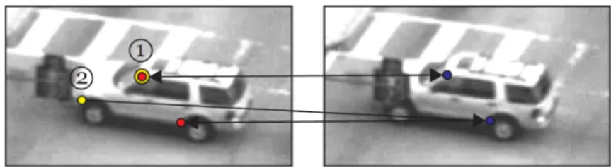
Kalal et al. [28] propose the forward-backward errormeasure. This error measure is conceptually illustrated in Fig.5. In the left image, the point1is tracked correctly to its corresponding position in the right image. The point2, however, ends up at a wrong location as an occlusion occurs. The proposed error measure is based on the idea that the tracking of points must be reversible. Point1is tracked back to its original location. In contrast, point 2 is tracked back to a different location. The proposed error measure is defined as the Euclidean distance
ε=|p−p00|,
wherep00is
p00=LK(LK(p)),
meaning that the Lucas-Kanade method is applied twice onp.
In [28] the forward-backward error measure is used in conjunction with another measure based on the similarity of the patch surroundingpand the patch surround-ing the tracksurround-ing resultp0. The similarity of these two patchesP andP is compared
Figure 5: The idea of the forward-backward error measure lies in the observa-tion that certain points cannot be re-tracked to their original locaobserva-tion. Images are from [28].
using the Normalised Correlation Coefficient (NCC) of two image patchesP1and P2that is defined as NCC(P1,P2) = 1 n−1 n
∑
x=1 (P1(x)−µ1)(P2(x)−µ2) σ1σ2 ,whereµ1,µ2,σ1 andσ2 are the means and standard deviations ofP1andP2. The
normalised correlation coefficient is invariant against uniform brightness varia-tions [32].
2.3 Transformation Model
Following the approach of Kalal et al. [28], we calculate the median of all forward-backward errors medFB and the median medNCC of all similarity measures and keep only those points exhibiting a forward-backward error less thanmedFB and a similarity measure larger thanmedNCC. Furthermore, if medFB is larger than a predefined thresholdθFB, we do not give any results as we interpret this case as an unreliable tracking result. The remaining points are used to calculate the trans-formation of the bounding box. For this, the pairwise distances between all points are calculated before and after tracking and the relative increase is interpreted as the change in scale. The translation in x-direction is computed using the median of the horizontal translations of all points. The translation in y-direction is calculated analogously. An algorithmic version of the proposed tracker is given in Alg.1. We use a grid of size 10×10, a window sizeW =10 and a thresholdθFB=10 for all of our experiments.
2.4 Summary
In this chapter we described the method that we employ for recursive estimation of an object of interest. No a priori information about the object is required except its position in the previous frame. We explained that the transformation of the bound-ing box of the previous frame is estimated by calculatbound-ing a sparse approximation to the optic-flow field and explain the method of Lucas-Kanade that we use for this estimation in detail. We introduced two error measures in order to improve
Algorithm 1Recursive Tracking Input: BI,I,J p1. . .pn←generatePoints(BI) for allpi do p0i←LK(pi) p00i ←LK(p0i) εi← |pi−p00i| ηi←NCC(W(pi),W(p0i)) end for medNCC←median(η1. . .ηn) medFB←median(ε1. . .εn) ifmedFB>θFBthen BJ =/0 else C← {(pi,p0i)|p 0 i6=/0,εi≤medFB,ηi≥medncc} BJ ←transform(BI,C) end if
Figure 6: Recursive tracking is possible as long as the selected object is visi-ble in the image. In the third frame an occlusion occurs. Images are from the SPEVI3dataset.
results and to act as a stopping criterion. In Fig.6an example result of this track-ing method is shown. In the left-most image, the initial boundtrack-ing box is depicted in blue. In the second image, it is shown that the selected object was tracked cor-rectly. By employing the stopping criterion, the method is able to identify when an occlusion takes place, as it is shown in the third image. However, in the fourth image the method is unable to re-initialise itself as it lacks a mechanism for object detection.
3
Detection
In this chapter we discuss the method that we employ for object detection. Ob-ject detection enables us to re-initialise the recursive tracker that itself does not maintain an object model and is therefore unable to recover from failure. While 3Surveillance Performance EValuation Initiative: http://www.eecs.qmul.ac.uk/
the recursive tracker depends on the location of the object in the previous frame, the object detection mechanism presented here employs an exhaustive search in order to find the object. Since several thousands of subwindows are evaluated for each input image, most of the time of our complete approach is spent for object detection.
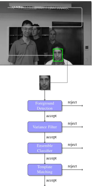
Our object detector is based on a sliding-window approach [49,16], which is illustrated in Fig.7. In this figure, the image at the top is presented to the object detector, which then evaluates a classification function at certain predefined sub-windows within each input image. Depending on the size of the initial object, we typically employ 50,000 to 200,000 subwindows for an image of VGA (640×480) resolution. Each subwindow is tested independently whether it contains the object of interest. Only if a subwindow is accepted by one stage in the cascade, the next stage is evaluated. The four stages that we use for image classification are shown below the input image. Cascaded object detectors aim at removing as many non-relevant subwindows with a minimal amount of computation [43]. First, we use a background subtraction method in order to restrict the search space to foreground regions only. This stage requires a background model and is skipped if it is not available. In the second stage all subwindows are rejected that exhibit a variance lower than a certain threshold. The third stage comprises an ensemble classifier based on random ferns [38]. The fourth stage consists of a template matching method that is based on the normalised correlation coefficient as a similarity mea-sure. We handle overlapping positive subwindows by employing a non-maximal suppression strategy.
This chapter is organised as follow. In Sec.3.1the sliding-window approach is described in detail. Sec.3.2shows how a background model restricts the search space to foreground regions. In Sec.3.3the variance filter is described. Sec.3.4 comprises a description of the ensemble classifier that is able rapidly identify pos-itive subwindows. The template matching method is described in Sec. 3.5. In Sec.3.6it is shown how overlapping detections are combined into a single result. In Sec3.7a summary of this chapter is given.
3.1 Sliding-Window Approach
In sliding-window-based approaches for object detection, subimages of an input image are tested whether they contain the object of interest [29]. Potentially, ev-ery possible subwindow in an input image might contain the object of interest. However, in a VGA image there are already 23,507,020,800 possible subwindows and the number of possible subwindows grows asn4 for images of sizen×n(see App. A.1for a proof), we restrict the search space to a subspace R by employ-ing the followemploy-ing constraints. We assume that the object of interest retains its aspect ratio. Furthermore, we introduce marginsdx anddy between two adjacent subwindows and set dx and dy to be 101 of the values of the original bounding box. In order to employ the search on multiple scales, we use a scaling factor s=1.2a,a∈ {−10. . .10}for the original bounding box of the object of interest.
Foreground Detection Variance Filter Ensemble Classifier Template Matching accept reject accept reject accept reject accept reject
Figure 7: In sliding-window-based approaches for object detection, subwindows are tested independently. We employ a cascaded approach in order to reduce com-puting time. The input image is from the SPEVI dataset.
We also consider subwindows with a minimum area of 25 pixels only. The size of the set of all subwindowsRconstrained in this manner is then
|R|=
∑
s∈1.2{−10...10} n−s(w+dx) sdx m−s(h+dx) sdy ,wherewandhdenote the size of the initial bounding box andnandmthe width and height of the image. A derivation for this formula is given in App.A.1. For an initial bounding box of size w=80 and h=60 the number of subwindows in a VGA image is 146,190. Since each subwindow is tested independently, we employ as many threads as cores are available on the system in order to test the subwindows.
3.2 Foreground Detection
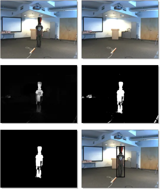
One approach in order to identify moving objects in a video stream is background subtraction, where each video frame is compared against a background model [13]. In this section, we describe how a background model speeds up the detection pro-cess. The problem of establishing a background model itself is non-trivial and out of scope for this work, for a survey see [39]. We perform background subtraction in four steps, as it is depicted in Fig.8. In this figure, the right upper image is the background imageIbgand the top left image is the imageI in which object detec-tion is to be performed. We start by calculating theabsolute differenceofIbgand
I
IabsDi f f =|Ibg−I|.
The result of this operation is shown in the first image of the second row. We now apply athresholdingof 16 pixels toIabsDi f f in order to create a binary image
Ibinary, which is shown in the second image of the second row.
Ibinary(x,y) =
(
1 ifIabsDi f f(x,y)>16 0 otherwise
In the following, we will refer to connected white pixels as components. In order to calculate the area and the smallest bounding box the blob fits into, we now apply thelabelingalgorithm proposed in [11]. This algorithm calculates labels in a single pass over the image. The idea of this algorithm is shown in Fig.9. Starting from the top row, each line is scanned from left to right. As soon as a white pixel A is encountered that is not yet labeled, a unique label is assigned to A and all the points lying on the contour of the component are assigned the same label as A. This contour is considered an external contour. This case is shown in the first image. If a pixelA0 on an external contour is encountered that is already labeled, all white pixels to the right are assigned the same label until another contour is encountered. If this is an external contour it is already labeled and the labeling algorithm proceeds. In the second image, this corresponds to to all the lines above
Figure 8: The process of background subtraction. From top left to bottom right: The input image, the background image, the result of the subtraction, the image after thresholding, after the removal of small components, the minimal bounding box around the foreground.
Figure 9: Labeling algorithm. Image is from [11].
pointB. If it is not yet labeled, as it is the case for the contour on whichBlies, then it considered an internal contour and all of its pixels are assigned the same label asB. This case is shown in the third image. If a labeled internal contour pointB0 is encountered, all subsequent white pixels are assigned the same label as A. This case is shown in the fourth image. The smallest bounding box the component fits into is determined by the coordinates of the outermost pixels of the component. The area of the component is the sum of all white pixels in a component.
Going back to Fig. 8, we now remove all components from the binary image with an area less than the size of the originally selected bounding box. The result of this operation is shown in the first image in the third row. All subwindows are rejected that are not fully contained inside one of the smallest bounding boxes around the remaining components. We call this set of bounding boxesC. If no background image is available, then all subwindows are accepted.
3.3 Variance Filter
The variance of an image patch is a measure for uniformity. In Fig.10two sample subwindows are shown, marked in red, that are evaluated in uniform background regions. Both of these subwindows contain patches that exhibit a variance lower than the patch of the object selected for tracking, which is contained in the right green rectangle. In this section we describe a mechanism that calculates the vari-ance of a patch in a subwindow using integral images and that rejects patches ex-hibiting a variance lower than a thresholdσmin2 . Such a variance filter is able to rapidly reject uniform background regions but unable to distinguish between dif-ferent well-structured objects. For instance, the left green bounding box in Fig.10 will be accepted as well.
We use an efficient mechanism in order to compute the variance that is shown in [49]. In order to simplify the following explanation, image patches defined by the bounding boxBare considered as a one-dimensional vector of pixels and its elements are addressed using the notationxi for theith pixel. For images, the varianceσ2is defined as σ2=1 n n
∑
i=1 (xi−µ)2, (2)Low Variance
High Variance
Figure 10: Uniform background regions are identified by setting a variance thresh-old.
wherenis the number of pixels in the image andµ is µ=1 n n
∑
i=1 xi. (3)An alternative representation of this formula is
σ2=1 n n
∑
i=1 x2i −µ2. (4)the derivation for this formula is given in App.A.2.
In order to calculateσ2 using Eq.4 for an image patch of sizen, nmemory lookups are needed. By taking advantage of the fact that two overlapping image patches partially share the same pixel values, we will now show a way to calculate
σ2 for an image patch that uses only 8 memory lookups after transforming the
input imageI into twointegral images. An integral imageI0 is of the same size asI and contains at location(x,y)the sum of all pixel values between the points
(1,1)and(x,y). This can be formulated as I0(x,y) =
∑
x0≤x,y0≤y
I(x0,y0). (5)
An integral image is computable in a single pass over the image by using the fact thatI0(x,y)can be decomposed into
I0(x,y) =I(x,y) +I0(x−1,y) +I0(x,y−1)−I0(x−1,y−1),
whereI0(x,y) =0 forx=0 ory=0. By using the integral image representation, the computation of the sum of pixels up to a specific point no longer depends on the number of pixels in the patch. In Fig. 11, the summed pixel values within the rectangleABCD is obtainable the following way. First, the sum of all pixels between(0,0)and the pointDis computed. Next, the pixels in the area between
(0,0) and B are subtracted as well as the pixels in the area between and(0,0)
andC. The area between(0,0)andAmust be added again, since it is subtracted twice. Using this observation, a formula for computing the sum of pixels within a bounding boxBconsisting of the parameters(x,y,w,h)is given by
n
∑
i=1
xi=I0(x−1,y−1)−I0(x+w,y−1)−I0(x−1,y+h) +I0(x+h,y+w). and use the notation
n
∑
i=1
xi=I0(B). (6)
as a shorthand. We use Eq.6in order to calculateµ in Eq.4. In order to calculate
also the first term of the right-hand side of this equation using integral images, we modify Eq.5to use the squared value ofI(x,y). We get
I00(x,y) =
∑
x0≤x,y0≤y
A B
C D
Figure 11: The sum of the pixel values within the rectangleABCD is calculable by summing up the pixels up toD, subtracting the pixels up to bothBandCand adding the pixels up toA. The computation is achieved using four look-ups when done on integral images.
In analogy to Eq.6we write n
∑
i=1
x2i =I00(B). (8)
By combining Eq.3, Eq.4, Eq.6and Eq.8, we get
σ2=1 nI 00 (B)− 1 nI 0 (B) 2 . (9)
This formula allows for a calculation ofσ2by using eight memory lookups. InA.3 the maximum resolution for integral images and typical data types are given. For
σmin2 , we use half of the variance value found in the initial patch.
3.4 Ensemble Classifier
In the third stage of the detection cascade we employ an ensemble classification method presented in [38] that is known asrandom fern classification. This clas-sifier bases its decision on the comparison of the intensity values of several pixels. For each tested subwindow, a probabilityPposis calculated. If this probability is smaller than 0.5 the subwindow is rejected. This method of classification is slower than the variance filter, but still is very fast compared to classification methods using SIFT features, as it was experimentally evaluated in [38].
We use features that are proposed in [31]. Fig.12depicts the process of feature calculation. In this figure, a sample image to be classified is shown. In each of the four boxes below this image, a black and a white dot are shown. Each of these dots refers to a pixel in the original image. The positions of these dots are drawn out of a uniform distribution once at startup and remain constant. For each of these boxes it is now tested whether in the original image the pixel at the position of the white dot is brighter than the pixel at the position of the black dot. Mathematically, we
1 1 0 1
F=13 Training Data
P(y=1|F) =0.9
Figure 12: Feature Calculation for a single fern. The intensity values of theith pixel pair determine theith bit of the feature value. This feature value is then used to retrieve the posterior probabilityP(y=1|Fk).
express this as
fi=
(
0 ifI(di,1)<I(di,2)
1 otherwise,
where di,1 and di,2 are the two random locations. Note that this comparison is
invariant against constant brightness variations. The result of each of these com-parisons is now interpreted as a binary digit and all of these values are concatenated into a binary number. In Fig.12the resulting binary number is 1101. When written in decimal form, this translates to 13, as it is shown in the box below the binary digit. Theith feature determines the value of theith bit of a number. In Alg.2, an algorithmic variant of this calculation is shown, in whichIis the input image,F is the calculated feature value andSis the number of features to be used. The value ofSinfluences the maximum feature value, which is 2S−1. A feature group of size S, such as the one shown in Fig.12 is referred to as afernin [38]. The obtained feature value is used to retrieve the probability P(y=1|F), wherey=1 refers to the event that the subwindow has a positive class label. These probabilities are determined by an online learning method that will be discussed in Chap.4.
Algorithm 2Efficient Fern Feature Calculation
Input: I Output: F F←0 fori=1. . .Sdo F←2×F ifI(di,1)<I(di,2)then F←F+1 end if end for
With only one fern, it is necessary to use a large number of features to achieve satisfactory results [38]. However, the amount of training data needed to estimate theP(y=1|Fk)increases with each additional feature. This problem is known as
curse of dimensionality[36]. Amit and Geman [3] encounter the same problem when using randomised decision trees for character recognition and alleviate it by not using one large tree, but several smaller trees. They then average their output. This finding was adopted in [38] and leads to the classifier depicted in Fig. 13. Below the image to be classified, there are three ferns, each consisting of a different set of feature positions and each yielding a different value forP(y=1|Fk). In the bottom rectangle, the average of these valuesPposis shown. Pposis expressed as
Ppos= 1 M M
∑
k=1 P(y=1|Fk),P(y=1|F1) =0.9 P(y=1|F2) =0.5 P(y=1|F3) =1.0
Ppos=0.8
Figure 13: Ensemble classification using three random ferns. The posteriorsP(y=
3.5 Template Matching
In the fourth stage of the detector cascade we employ a template matching method. This stage is even more restrictive than the ensemble classification method de-scribed in the previous section, since the comparison is performed on a pixel-by-pixel level. We resize all patches to 15×15 pixels. For comparing two patchesP1
andP2, we employ the Normalised Correlation Coefficient (NCC) ncc(P1,P2) = 1 n−1 n
∑
x=1 (P1(x)−µ1)(P2(x)−µ2) σ1σ2 ,whereµ1,µ2,σ1 andσ2are the means and standard deviations ofP1 andP2. This
distance measure is also known as the Pearson coefficient [40]. When interpreted geometrically, it denotes the cosine of the angle between the two normalised vec-tors [10]. NCC yields values between−1 and 1, with values closer to 1 when the two patches are similar. We use the following formula in order to define a distance between two patches that yields values between 0 and 1.
d(P1,P2) =1−
1
2(ncc(P1,P2) +1).
We maintain templates for both the positive and negative class. We refer to the positive class asP+ and to the negative class asP−. The templates are learned online, as it will be described in Sec.4.2. In Fig.14positive and negative examples are shown that were learned on the sequenceMulti Face Turning(see Sec.5.4for a description). Given an image patchPthat is of unknown class label, we calculate both the distances to the positive class
d+= min
Pi∈P+d(P0,Pi)
and the distance to the negative class d−= min
Pj∈P−
d(P0,Pj).
In Fig.15, the green dots correspond to positive instances and red dots correspond to negative instances. The black dot labeled with a question mark corresponds to a patch with unknown class label. The distance to the nearest positive instance is d+=0.1 and the distance to the nearest negative instance is d−=0.4. We fuse these distances into a single value using the formula
p+= d
−
d−+d+
that expresses the confidence whether the patch belongs to the positive class. A subwindow is accepted if p+ is greater than a threshold θ+. A confidence value
above this threshold indicates that the patch belongs to the positive class. We use a value of θ+ =0.65 for all of our experiments. In Fig. 16, p+ is shown for all possible values. As it can be seen from this figure, p+ is 1 if d+ is 0. This corresponds to the event that an exact positive match has been found. Ifd− is 0,
(a) Positive Examples (b) Negative Examples
Figure 14: Positive and negative patches acquired for the template matching method during a run on a sequence from the SPEVI dataset.
d+=0.1 d−=0.4 ?
Figure 15: An unknown patch, labeled with a question mark, and the distanced+ to the positive class and the distanced−to the negative class. The distance is based on the normalised correlation coefficient. The actual space in which the distance measurement takes place has 15×15 dimensions.
0 0.5 1 0 0.5 1 0 0.5 1 d -d+ 0 0.2 0.4 0.6 0.8 1
Figure 16: The confidence for a patch being positive depends on the distance to the closest positived+and on the distance to the closest negative patchd−.
Figure 17: Overlapping subwindows with high confidence (yellow) are averaged and form a single result (green). The underlying image is from [41].
3.6 Non-maximal Suppression
So far, the components of the detector cascade were introduced. Each subwindow is assigned a valuep+that expresses the degree of belief whether it contains the ob-ject of interest. According to Blaschko [7], an object detection mechanism ideally identifies positive subwindows with a confidence value of 1 and negative subwin-dows with a confidence of 0, but in practice the output consists of hills and valleys characterizing intermediate belief in the fitness of a given location. In Fig.17this situation is illustrated. In this figure, several detections with high confidence occur around the true detection marked in green. Blaschko also states that considering only the subwindow yielding the highest confidence is problematic because this leads to other local maxima being ignored. Instead it is desirable to employ non-maximal suppressionstrategies that identify relevant local maxima.
B1
B2
I
Figure 18: We define an overlap measure between two bounding boxesB1 and
B2 to be the area of their conjunction I divided by the area of their disjunction
B1+B2−I.
For non-maximal suppression, we use the method described in [49] that clus-ters detections based on their spatial overlap. For each cluster, all bounding boxes are then averaged and compressed into a single detection. The confidence value p+of this single bounding box is then the maximum value confidence value in the corresponding cluster. In Fig.18,B1 is the area of the first bounding box,B2 the
area of the second bounding box andI is the area of the intersection of the two bounding boxes. For measuring the overlap between two bounding boxes, we use the formula from the PASCAL challenge [18]
overlap=B1∩B2
B1∪B2 =
I
(B1+B2−I). (10)
This measure is bounded between 0 and 1. We now use thehierarchical clustering
algorithm described in [37] that works as follows. First we calculate the pairwise overlap between all confident bounding boxes. We then start at one bounding box and look for the nearest bounding box. If this distance is lower than a certain cutoff threshold, we put them into the same cluster and furthermore, if one of the bounding already was in a cluster, we merge these clusters. If the overlap is larger than the cutoff threshold, we put them into different clusters. We then proceed to the next bounding box. We use a cutoff of 0.5 for all of our experiments.
3.7 Summary
In this chapter, we described how we run a cascade object detector on a subset of all possible subwindows in an input image. The components of the detection cascade were described and it was shown how overlapping positive bounding boxes are grouped into a single detection by employing non-maximal suppression. We ex-plained that the foreground detector and the variance filter are able to rapidly reject subwindows, but require a preprocessing step. The ensemble classifier is compu-tationally more expensive but provides a more granular decision mechanism. The final decision is obtained by comparing each subwindow to normalised templates. In Table1it is shown for each component how many memory lookups are neces-sary in order to test a subwindow.
Method Memory Lookups
Foreground Detection |C|
Variance Filter 8
Ensemble Classifier 2·M·S Template Matching 255· |P+| · |P−|
Table 1: Comparison of necessary memory lookups for testing a subwindow. The variance filter and the ensemble Classifier operate at constant time (M andS are constant values). The foreground detection depends on the number of detected foreground regions |C|. The template matching method depends on the learned number of templates.
In Alg. 3 an algorithm for implementing the detection cascade is given. In Line1the setDt that contains confident detection is initialised. In Lines2-4the re-quired preprocessing for the foreground detection and the variance filter is shown. Lines5-16contain the actual cascade. In Line11the subwindow is added to the set of confident detections if it has passed all stages of the cascade. In Line17the non-maximal suppression method is applied.
Algorithm 3Detection Cascade 1: Dt ←/0 2: F←foreground(I); 3: I0←integralImage(I); 4: I00←integralImage(I2); 5: for allB∈Rdo 6: ifisInside(B,F);then
7: ifcalcVariance(I0(B),I00(B))>σmin2 then
8: ifclassifyPatch(I(B))>0.5then 9: P←resize(I(B),15,15) 10: ifmatchTemplate(I(B))>θ+then 11: Dt←DtSB 12: end if 13: end if 14: end if 15: end if 16: end for 17: Dt ←cluster(Dt)
4
Learning
When processing an image, both the recursive tracker and the object detector are run in parallel. In this chapter we deal with the question of how to combine the output of both methods into a single final result. We then show what happens during the learning step and when it is performed.
The background model and the threshold for the variance filter are not adapted during processing, while the ensemble classifier and the template matching method are trained online. We address the template update problem by defining certain criteria that have to be met in order to consider a final result suitable for performing a learning step. In learning, we enforce two P/N-learning constraints [27]. The first constraint requires that all patches in the vicinity of the final result must be classified positively by the object detector. The second constraint requires that all other patches must be classified negatively by the object detector.
This remainder of this chapter is organised as follows. In Sec.4.1it is shown how the results of the recursive tracker and the object detector are combined. Fur-thermore, the criteria for validity are given. In Sec. 4.2 it is explained how the constraints are implemented. In Sec.4.3 the main loop of our approach is given. Sec.4.4concludes this chapter with a summary.
4.1 Fusion and Validity
In Alg. 4 our algorithm for fusing the result of the recursive tracker Rt and the confident detectionsDt into a final resultBt is given. The decision is based on the number of detections, on their confidence valuesp+Dt and on the confidence of the tracking resultp+R
t. The latter is obtained by running the template matching method on the tracking result. If the detector yields exactly one result with a confidence higher than the result from the recursive tracker, then the response of the detector is assigned to the final result (Line5and15). This corresponds to are-initialisation
of the recursive tracker. If the recursive tracker produced a result and is not re-initialised by the detector, either because there is more than one detection or there is exactly one detection that is less confident than the tracker, the result of the recursive tracker is assigned to the final result (Line7). In all other cases the final result remains empty (Line1), which suggests that the object is not visible in the current frame.
We use the predicatevalid(Bt)to express a high degree of confidence that the final resultBt is correct. Only if the final result is valid the learning step described in the next section is performed. As it is stated in Alg.4 the final result is valid under the following two circumstances, both of which assume that the tracker was not re-initialised by the detector. The final result is valid if the recursive tracker produced a result with a confidence value being larger than θ+ (Line 9). The
final result is also valid if the previous result was valid and the recursive tracker produced a result with a confidence larger thanθ−. (Line11). In all other cases,
already in Sec.3.5, the thresholdθ+indicates that a result belongs to the positive class. The thresholdθ−indicates that a result belongs to the negative class and is
fixed atθ−=0.5 for all of our experiments. Algorithm 4Hypothesis Fusion and Validity.
Input: Rt,Dt Output: Bt 1: Bt ← /0 2: valid(Bt)←false 3: ifRt 6=/0then 4: if|Dt|=1∧p+Dt >p + Rt then 5: Bt ←Dt 6: else 7: Bt ←Rt 8: if p+R t >θ +then 9: valid(Bt)←true 10: else ifvalid(Bt−1)∧p+Rt >θ −then 11: valid(Bt)←true 12: end if 13: end if 14: else if|Dt|=1then 15: Bt←Dt 16: end if 4.2 P/N-Learning
According to Chapelle [12], there are two fundamentally different types of tasks in machine learning. Insupervised learninga training set is created and divided into classes manually, essentially being a set of pairshxi,yii. Thexi correspond to training examples and theyi to the corresponding class label. The training set is used to infer a function f :X→Y that is then applied to unseen data. Supervised learning methods in object detection have been successfully applied most notably to face-detection [49] and pedestrian detection [16]. However, the learning phase prevents applications where the object to be detected is unknown beforehand. In the same way, the learned classifier is also unable to adapt to changes in the distri-bution of the data. The second task in machine learning isunsupervised learning. In this setting, no class labels are available and task is finding a partitioning of this data, which is be achieved by density estimation, clustering, outlier detection and dimensionality reduction [12].
Between these two paradigms there is semi-supervised learning. In semi-supervised learning, there are labeled examples as well as unlabeled data. One type of semi-supervised learning methods uses the information present in the training data as supervisory information [12] in order to find a class distribution in the
Figure 19: P/N Constraints
unlabeled data and to update the classifier using this class separation as a training set. In our tracking setting there is exactly one labeled example. In [27], a semi-supervised learning method calledP/N-learningis introduced. This method shows how so-called structural constraints can extract training data from unlabeled data for binary classification. In P/N-learning, there are two types of constraints: A P-constraint identifies false negative outputs and adds them as positive training examples. An N-constraint does the converse. In Fig.19,Xurefers to the unlabeled data available. This data is first classified by an existing classifier that assigns labels Yu to Xu. Then, the structural constraints, according to some criterion, identify misclassified examples Xc with new labelsYc. These examples are then added to the training set and training is performed, which results in an update of the classification function.
We use the following constraints for object detection that are proposed in [27]. The P-Constraint requires that all patches that are highly overlapping with the final result must be classified as positive examples. The N-Constraint requires that all patches that are not overlapping with the valid final result must be classified as negative examples. We consider a bounding boxBhighly overlapping withBt if it exhibits an overlap of at least 60%. Bis considered not to be overlapping withBt if the overlap is smaller than 20%. For measuring overlap, we employ the metric already described in Sec.3.6.
A complete algorithmic description of the constraints is given in Alg.5. We will now describe the measures that we take in order to adapt the ensemble clas-sifier and the template matching method in order to classifiy these examples cor-rectly. For the ensemble classifier, we have not yet explained how the posterior values are calculated for each fern. Recall thatP(y=1|Fk) is the probability
whether a patch is positive given the featuresFk. We define the posterior to be
P(y=1|Fk) =
( pFk
pFk+nFk, ifpFk+nFk >0 0, ifpFk+nFk =0.
In this formulapFk is the number of times the P-constraint was applied to this com-bination of features andnFk is the number of times the N-constraints was applied. In Line2we test whether a bounding box overlapping with the final result is mis-classified by the ensemble classifier. We incrementpFkin Line5for each fern if the overlap is smaller than 0.6 and the ensemble classifier yielded a confidence lower than 0.5. In Line10nFk is incremented for misclassified negative patches. When updating the ensemble classifier, the computational overhead does not increase. This is different for the template matching method, as every additional patch in the set of positive or negative templates increases the number of comparisons that must be made in order to classify a new patch. In order to change the label of a misclassified positive patch for the template matching method, we add it to the set of positive templates. This patch then has a distance ofd+=0, which means that its confidence is 1. However, as it is shown in Line18, we do this only for the patch contained in the final resultBt. Note that the learning step is performed only if the final result is valid, which already implies thatp+Bt is larger thanθ−. As
for the N-constraint for the template matching method, we add negative patches to the template matching method if they were misclassified by the ensemble classifier and also are misclassified by the template matching methods.
In Fig.20it is illustrated when positive templates are added. At point A, track-ing starts with a high confidence and a valid result. Learntrack-ing is performed, but no positive examples are added, because the confidence is aboveθ+. The confidence then drops belowθ+ (Point B) but remains aboveθ−. According to Alg.4 this
means that the final result is still valid. Exactly in this case positive patches are added, which leads to an increased confidence. At Point C, the confidence drops belowθ−, which leads to the final result not being valid anymore. In Point D,
confidence is at the same level as in Point B, but no learning is performed since the final result is not valid.
4.3 Main Loop
We now have described all components that are used in our approach. In Alg.6 the main loop of our implementation is given. When the initial patch is selected, a learning step is performed (Line1). For each image in the sequence, the tracker and the detector are run (Line3and4), their result is fused (Line5) and if the final result is considered valid then the learning step is performed (Line7). The final result is then printed (Line9) and the next image is processed.
Algorithm 5Applying P/N-constraints
Input: I,Bt
1: for allB∈Rdo
2: ifoverlap(B,Bt)>0.6andclassifyPatch(I(B))<0.5then 3: fork=1. . .Mdo
4: F←calcFernFeatures(I(B),k)
5: pFk[F]←pFk[F] +1 6: end for
7: else ifoverlap(B,Bt)<0.2andclassifyPatch(I(B))>0.5then 8: fork=1. . .Mdo 9: F←calcFernFeatures(I(B),k) 10: nFk[F]←nFk[F] +1 11: end for 12: if p+B t >θ −then 13: P−←P−∪I(B) 14: end if 15: end if 16: end for 17: ifp+Bt <θ+then 18: P+←P+∪I(Bt) 19: end if 0 θ− θ+ 1 A B C D Frame Confidence
Figure 20: Positive examples are added only when the confidence value drops from a high value (FrameA) to a value betweenθ+ andθ−(Frame B). In FrameDno learning is performed, since the confidence rises from a low value in FrameC. This measure ensures that the number of templates is kept small.
Algorithm 6Main loop Input: I1. . .In,B1 1: learn(I1,B1) 2: fort=2. . .ndo 3: Rt←track(It−1,It,Bt−1) 4: Dt ←detect(It) 5: Bt←fuse(Rt,Dt) 6: ifvalid(Bt)then 7: learn(It,Bt) 8: end if 9: print(Bt) 10: end for 4.4 Summary
In this chapter, we described that we obtain a final result based on the results of the recursive tracker and the object detector by basing our decision on the confidence of the template matching method run on both results. We further defined criteria for validity based on the confidence value and of the validity of the previous bounding box. We perform learning only if the final result is valid. The learning step consists of identifying falsely labeled examples and updating the ensemble classifier and the template matching method in order to correctly classify them.
5
Results
In this chapter, our approach is evaluated empirically both on sequences that have been used in the literature as well as on newly recorded sequences. We employ the standard metrics recall and precision for assessing performance. For this evalua-tion, a C++ implementation was created, where the calculation of the optical flow (Sec.2.1), the calculation of the normalised correlation coefficient (Seq. 3.5), all the operations for the foreground detection (Sec.3.2) as well as low-level image operations are implemented as function calls to the OpenCV4library. The multi-threaded optimisation described in Sec.3.1 was implemented using an OpenMP5 pragma. All experiments were conducted on an Intel Xeon dual-core processor running at 2.4 Ghz.
This chapter is organised as follows. Sec.5.1explains the evaluation protocol. In Sec.5.2, the video sequences that are used in our experiments are described. In Sec.5.3, the parameters for the ensemble classifier are evaluated empirically. In Sec.5.4, qualitative results are shown on two video sequences. The requirement set on the overlap when comparing to ground truth is discussed in Sec.5.5. In Sec.5.6
4Open Computer Vision:http://opencv.willowgarage.com 5Open Multi-Processing:http://openmp.org
quantitative results for performance and execution time are obtained for our ap-proach and two state-of-the-art methods. In Sec.5.7our algorithm is evaluated in a multi-camera scenario. Each experiment is concluded with a discussion.
5.1 Evaluation Protocol
In order to compare the output of an algorithm to ground truth values we use the overlap measure from Eq.10. In [24] it is shown that this measure equally penalizes translations in both directions and scale changes. Based on the overlap between algorithmic output and ground truth values, each frame of a sequence is categorised as one of the five possible cases shown in Fig. 21. A result is considered true positiveif the overlap is larger than a thresholdω (Casea). A result is counted as false negativewhen the algorithm yields no result for a frame even though there is an entry in the ground truth database (Caseb). The opposite case is afalse positive
(Casec). If the overlap is lower than the thresholdω, then this is counted both a
false negative and a false positive (Cased). If for a frame neither an algorithmic output nor an entry in the ground truth database exists then this case is considered atrue negative(Casee).
After processing a video sequence, all occurrences of True Positives (TP), False Positives (FP), True Negatives (TN) and False Negatives (FN) are counted. Based on these values we calculate two performance metrics. Recall is defined as
recall= TP
TP+FN
and measures the fraction of positive examples that are correctly labeled [17]. Pre-cision is defined as
precision= TP
TP+FP
and measures the fraction of examples classified as positive that are truly posi-tive [17]. Depending on the application, high recall or high precision (or both) may be demanded. Since our approach uses random elements, we repeat every experiment five times and average the values for precision and recall.
Our algorithm provides a confidence measure for each positive output it pro-duces. By applying thresholding, results exhibiting a confidence lower than a cer-tain valueθ are suppressed. This suppression affects the performance metrics as
follows. True positives with a confidence less thanθbecome false negatives, mean-ing that both recall and precision get worse. Also, false positives with a confidence less thanθ become true negatives, meaning that precision improves. Thresholding
is most effective if false positive results are produced with low confidence values and true positive results with high confidence values. A precision-recall curve vi-sualise how different values forθ impact precision and recall. A sample curve is
given in Fig. 22, where the right bottom end of the curve refers to the precision and recall values when the threshold is 0, meaning that no true positives and no false positives were removed. The rest of the curve represents recall and preci-sion values asθ is increased, ending in a point whereθ=1. We chose not to use
GT
ALG
(a) True Positive
GT
(b) False Negative
ALG
(c) False Positive
GT ALG
(d) False Negative and False Positive
(e) True Negative
Figure 21: Five possible cases when comparing algorithmic results to ground truth values. The case(e)is not considered in metrics that we use.
precision-recall curves because it turned out during experiments that no relevant improvement for precision was achievable. We attribute this to the mechanism for automatic failure detection described in Sec.2.3that prevents false positives.
0 0.5 1 0 0.5 1 Recall Precision
Figure 22: Sample precision-recall curve.
5.2 Sequences
In this section we describe the sequences that we use for evaluation, all of which are accompanied by manually annotated ground truth data. Multi Face Turning
from the SPEVI6dataset consists of four people moving in front of a static camera, undergoing various occlusions and turning their faces right and left. The diffi-culty in this sequence lies in the fact that four instances of the same category are present and that all persons undergo various occlusions. The sequence consists of 1006 individual frames. The sequence PETS view 001is taken from the PETS 20097 dataset. It shows pedestrians walking across a T junction and consists of 794 frames. The pedestrians exhibit a similar appearance due to low spatial reso-lution. The following six sequences that are shown in Fig.23were used in [51,27] for evaluating object tracking methods. The sequenceDavid Indoor8consists of 761 frames and shows a person walking from an initially dark setting into a bright room. No occlusions occur in this sequence. Jumping consists of 313 frames and shows a person jumping rope, which causes motion blur. Pedestrian 1 (140 frames),Pedestrian 2(338 frames) andPedestrian 3(184 frames) show pedestri-ans being filmed by an unstable camera. The sequenceCarconsists of 945 frames showing a moving car. This sequence is challenging because the images exhibit low contrast and various occlusions occur.
6Surveillance Performance EValuation Initiative: http://www.eecs.qmul.ac.uk/
~andrea/spevi.html
7Performance Evaluation of Tracking and Surveillance: http://www.cvg.rdg.ac.uk/
PETS2009/a.html
(a) David Indoor (b) Jumping (c) Pedestrian 1
(d) Pedestrian 2 (e) Pedestrian 3 (f) Car
Figure 23: The data set used for analysing the importance of the overlap measure and for comparing to existing approaches.
We recorded two datasets, Multi Cam Narrow andMulti Cam Wide, each consisting of three sequences, for the evaluation in multi-camera scenarios. The camera positions and orientations for both datasets are shown in Fig.24. InMulti Cam Narrowthe cameras were placed next to each other, each camera looking in the same direction. For Multi Cam Wideeach camera was placed in a corner of the room, facing to its center. In Fig.25a frame from each camera inMulti Cam Wideis shown recorded at the same instant of time. In Fig.26a frame from each sequence inMulti Cam Wide is shown as well as enlarged views of the selected object.
5.3 Parameter Selection for Ensemble Classifier
In this experiment we analyse the effects of varying the parameters for the ensem-ble classifier on the sequenceMulti Face Turning. The two parameters in question are the number of features in a group (S) and the total number of groups (M). In [38] it was concluded that settingS=10 andM=10 gives good recognition rates. Since we do not employ random ferns as a final classification step but as part of a detector cascade and furthermore use on online learning approach, we re-evaluate these parameters. Breiman [9] shows that randomized decision trees do not overfit as the number of trees is increased but produce a limiting value of the generalization error. This means that increasingMdoes not decrease recall.
Since Sis the number of features that are assumed to be correlated, for large values ofSthe curse of dimensionality arises, meaning that the amount of training data increases withS. On the other hand, low values ofSignore correlation in the
3 1 2
(a) Multi Cam Narrow
3 1 2
(b) Multi Cam Wide Figure 24: Camera setup forMulti Cam Narrow.
Figure 26: Sample frames ofMulti Cam Wideand an enlarged view of the selected object.
data [38]. Another aspect for choosingSis the amount of memory required. For S=24, at least 16,777,216 entries for the posterior values have to be stored for every fern. For this experiment, we setM=50 and letS vary from 1 to 24. In Fig.27,Sis plotted against the achieved recall. The recall first increases linearly withSand reaches its maximum at S=13. For higher values ofS, less recall is achieved.
Since the time spent on testing each sliding window depends linearly onM, this means that M should be small when low execution time is desired. Fig.28 shows how the recall is affected byM. For this experiment, we set S=13. The results show that recall increases up toM=30 and does not change afterwards.
Discussion
This experiment shows that the parameters of the ensemble classifier influence recall. We get best results forS=13 andM>30. The observations here are in line with the finding in [9] that randomised decision trees do not overfit as more trees are added. For the rest of the experiments in this chapter, we setS=13 and M=10, as a compromise between recall, speed and memory consumption.
0 10 20 0 0.5 1 S Recall
Multi Face Turning
Figure 27: Varying the sizeSof the feature groups whenM=50.
0 20 40 60 80 100 120 140 160 180 200 0 0.5 1 M Recall
Multi Face Turning
5.4 Qualitative Results
In this section, qualitative results for the sequencesMulti Face TurningandPETS view 001are given. In all of the presented images, a blue bounding box denotes a result with its confidence being larger than 0.5, all other bounding boxes are drawn in yellow. We show results forMulti Face Turningin Fig.29. In the top left image, the face initially selected for tracking is shown. The person then moves to the right and gets occluded by another person. The recursive tracker correctly stops tracking and the face is detected as it appears to the right of the occluding person. This is shown in the top right image. The selected face then turns left and right several times and undergoes another occlusion, which is again handled correctly, as it is depicted in the first image in the second row. The selected person then leaves the camera view on the right and enters on the same side in the back of the room. At first, the head of the person is rotated but as soon as a position frontal to the camera is assumed a detection occurs, as it is shown in the second image in the second row. In the first image in the third row the recursive tracker does not stop tracking even though an occlusion occurred, however no learning is performed since the distance to the model remains below 0.5, as indicated by the yellow bounding box. The detector then yields a detection with a higher confidence than the recursive tracker, as it is depicted in the second image in the third row. The person then leaves the field of view on the left-hand side and enters at a position close to the camera (see first image in the fourth row), appearing twice as large as in the first frame. The face is detected and tracked correctly until the last appearance of the selected face, depicted in the second image in the fourth row.
Results for PETS view 001 are shown in Fig. 30. The person shown in the top-left image is selected for tracking. The person walks to the left and gets almost fully occluded several times by the pole in the middle of the image. Additional occlusions occur when walking behind two other people. The tracker stops and the detector correctly re-initialises the target as soon as it reappears, which is shown in the second image in the first row. The person then returns to the right-hand side of the image and leaves the field of view while being tracked correctly, as it is depicted in the first image of the second row. In the second image of the second row a false detection occurs. The original target then appears on the right-hand side of the field of view and causes another detection, as it is shown in the first image of the third row. The person then walks to the left and gets occluded by another person, as depicted in the second image in the third row. Both persons walk in opposite directions, which causes the recursive tracker to erroneously remain at the current position for the following 297 frames with a confidence lower than 0.5. The target person in the meantime walks around the scene without being re-detected. Finally, a correct detection occurs in the last image presented and the person is tracked correctly until the end of the sequence.
Discussion
The experiments discussed in this section demonstrate that our method is able to learn the appearance of objects online and to re-detect the objects of interest after occlusions, even at different scales. OnMulti Face Turning, the face is re-detected after every but one occlusion. In both the first and the second experiment there are frames where the object of interest is not detected even though it is visible. InMulti Face Turningthis is due to the face appearing in a pose that never appeared before, which is a situation that our method cannot handle. In the second experiment, the object of interest is not detected even it appears in poses similar to the ones encountered in learning steps. The problem here is that during learning, the other persons walking around the scenes are (correctly) recognised as negative examples. However, since the appearance of these persons is similar to the appearance of the object of interest, a close positive match is needed in order to achieve a detection. InMulti Face Turningthe faces exhibit sufficiently dissimilarity.
5.5 Requirement on Overlap
As it was pointed out in Sec.5.1, the categorisation of algorithmic output depends on the parameterω that defines the required overlap between an algorithmic result
and ground truth values. Whenω is increased, both recall and precision decrease.
Depending on the intended application, different requirements on accurate results are desired. In this section we analyse empirically to what extent precision and recall change when varyingω. For this experiment, we use three different values
forω (0.25, 0.5 and 0.75) and evaluate precision and recall on the sequencesDavid Indoor, Jumping, Pedestrian 1-3andCar. The resulting values for precision and recall that are obtained when running our implementation with the three different values forω are shown in Table2.
omega=0.75 omega=0.5 omega=0.25
David Indoor 0.08/0.08 0.65/0.65 0.66/0.66 Jumping 0.13/0.14 0.63/0.63 1.00 1.00 Pedestrian 1 0.00/0.00 0.04/0.04 1.00 1.00 Pedestrian 2 0.06/0.11 0.55/1.00 0.56/1.00 Pedestrian 3 0.22/0.35 0.32/0.51 0.32/0.51 Car 0.08/0.09 0.95/0.94 0.95/0.94
Table 2: Performance metrics improve when the requirement on the overlapω is relaxed. The first value in a cell denotes recall, the second value is precision.
Discussion
In the conducted experiment, for all sequences there is a drastic increase in both recall and precision when the requirement of an exact match is relaxed. This is
![Figure 9: Labeling algorithm. Image is from [11].](https://thumb-us.123doks.com/thumbv2/123dok_us/1962881.2790751/16.892.166.731.186.320/figure-labeling-algorithm-image-is-from.webp)