and Data Management,
2nd Edition
A Guide for SPSS
®and SAS
®Users
Raynald Levesque
Chicago, IL 60606-6412 Tel: (312) 651-3000 Fax: (312) 651-3668
SPSS is a registered trademark and the other product names are the trademarks of SPSS Inc. for its proprietary computer software. No material describing such software may be produced or distributed without the written permission of the owners of the trademark and license rights in the software and the copyrights in the published materials.
The SOFTWARE and documentation are provided with RESTRICTED RIGHTS. Use, duplication, or disclosure by the Government is subject to restrictions as set forth in subdivision (c)(1)(ii) of The Rights in Technical Data and Computer Software clause at 52.227-7013. Contractor/manufacturer is SPSS Inc., 233 South Wacker Drive, 11th Floor, Chicago, IL 60606-6412.
General notice: Other product names mentioned herein are used for identification purposes only and may be trademarks of their respective companies.
SAS is a registered trademark of SAS Institute Inc.
Windows is a registered trademark of Microsoft Corporation. Microsoft® Access, Microsoft® Excel, and Microsoft® Word are products of Microsoft Corporation.
DataDirect, DataDirect Connect, INTERSOLV, and SequeLink are registered trademarks of DataDirect Technologies. Portions of this product were created using LEADTOOLS © 1991–2000, LEAD Technologies, Inc.
ALL RIGHTS RESERVED.
LEAD, LEADTOOLS, and LEADVIEW are registered trademarks of LEAD Technologies, Inc. Portions of this product were based on the work of the FreeType Team (http://www.freetype.org).
A portion of the SPSS software contains zlib technology. Copyright © 1995–2002 by Jean-loup Gailly and Mark Adler. The zlib software is provided “as-is,” without express or implied warranty. In no event shall the authors of zlib be held liable for any damages arising from the use of this software.
A portion of the SPSS software contains Sun Java Runtime libraries. Copyright © 2003 by Sun Microsystems, Inc. All rights reserved. The Sun Java Runtime libraries include code licensed from RSA Security, Inc. Some portions of the libraries are licensed from IBM and are available at http://oss.software.ibm.com/icu4j/. Sun makes no warranties to the software of any kind.
Sax Basic is a trademark of Sax Software Corporation. Copyright © 1993–2004 by Polar Engineering and Consulting. All rights reserved.
SPSS® Programming and Data Management, 2nd Edition: A Guide for SPSS® and SAS® Users Copyright © 2005 by SPSS Inc.
All rights reserved.
Printed in the United States of America.
No part of this publication may be reproduced, stored in a retrieval system, or transmitted, in any form or by any means, electronic, mechanical, photocopying, recording, or otherwise, without the prior written permission of the publisher. 1 2 3 4 5 6 7 8 9 0 06 05 04 03
iii
P r e f a c e
Experienced data analysts know that a successful analysis or meaningful report often requires more work in acquiring, merging, and transforming data than in specifying the analysis or report itself. SPSS contains powerful tools for accomplishing and
automating these tasks. While much of this capability is available through the graphical user interface, many of the most powerful features are available only through command syntax, the macro facility that extends the power of command syntax, and the scripting facility. Until now, no book or other documentation has focused on those features, and many potential users have been unaware of the power available to them or have not exploited it for lack of examples. This book fills that void.
Using This Book
The contents of this book and the accompanying CD are discussed in Chapter 1. In particular, see the section “Using This Book” if you plan to run the examples on the CD. The CD also contains additional command files, macros, and scripts that are mentioned but not discussed in the book and that can be useful for solving specific problems.
This edition has been updated to included numerous enhanced data management features introduced in SPSS 13.0. Many examples will work with earlier versions, but some examples rely on features not available prior to SPSS 13.0.
For SAS Users
If you have more experience with SAS than with SPSS for data management, see Chapter 10 for comparisons of the different approaches to handling various types of data management tasks. Quite often, there is not a simple command-for-command relationship between the two programs, although each accomplishes the desired end.
iv
the book (not the software) to [email protected]. Check my Web site at www.spsstools.net for possible errata and generalizations or improvements of code included on the companion CD.
Acknowledgments
First of all, I wish to thank the SPSS Senior Director of Publications, Bob Gruen, for giving me the opportunity to work on this challenging project. In addition to providing general guidance, Bob reviewed the macros chapter. Jon Peck reviewed and
contributed to the scripting chapter. Richard Cohen provided a new chapter on scoring. In addition to reviewing all of the remaining chapters, Rick Oliver wrote the sections on importing data from sources other than text files, data transformations, and the new SPSS Output Management System. I enjoyed working with these gentlemen; the book greatly benefited from their technical expertise and communications skills.
I also wish to thank Stephanie Schaller, who provided many sample SAS jobs and helped to define what the SAS user would want to see, as well as Marsha Hollar and Brian Teasley, the authors of the chapter“SPSS for SAS Programmers.”
On the nontechnical side, I am grateful to my spouse, Nicole Tousignant, who demonstrated patience and provided support and encouragement during those months when I was handling two jobs and working seven days a week. I dedicate this book to her.
v
1 Overview
1
Data Management Tasks . . . . 1
Using SPSS Data Management Facilities . . . . 3
Graphical User Interface. . . . 3
Command Language . . . . 4
Macro Facility . . . . 5
Scripting Facility . . . . 5
Working with Command Syntax . . . . 5
Creating Command Syntax Files . . . . 5
Running SPSS Commands . . . . 6
Syntax Rules. . . . 7
Using This Book . . . . 8
Documentation Resources . . . . 8
2 Best Practices and Efficiency Tips
11
Introduction . . . 11Customizing the Programming Environment . . . 11
Displaying Commands in the Log . . . 11
Displaying the Status Bar in Command Syntax Windows . . . 12
Customizing the Toolbars . . . 13
Protecting the Original Data . . . 16
Do Not Overwrite Original Variables . . . 16
Using Temporary Transformations . . . 17
Using Temporary Variables . . . 18
Using Command Syntax to Document Work . . . 20
vi
MISSING VALUES Command . . . 24
WRITE and XSAVE Commands . . . 25
Using Comments . . . 25
Using SET SEED to Reproduce Random Samples or Values . . . 25
Divide and Conquer . . . 27
Using INSERT with a Master Command Syntax File . . . 27
Defining Global Settings . . . 28
3 Getting Data into SPSS
33
Getting Data from Databases . . . 33Installing Database Drivers . . . 33
Database Wizard . . . 34
Reading a Single Database Table . . . 35
Reading Multiple Tables . . . 37
Reading Excel Files . . . 40
Reading a “Typical” Worksheet . . . 40
Reading Multiple Worksheets. . . 43
Reading Text Data Files . . . 45
Simple Text Data Files . . . 46
Delimited Text Data. . . 47
Fixed-Width Text Data . . . 51
Text Data Files with Very Wide Records. . . 55
Reading Different Types of Text Data . . . 56
Reading Complex Text Data Files . . . 58
Mixed Files . . . 58
Grouped Files . . . 59
Nested (Hierarchical) Files . . . 62
Repeating Data . . . 68
vii
Variable Labels. . . .77
Value Labels . . . .77
Missing Values . . . .78
Measurement Level . . . .79
Using Variable Properties As Templates . . . .79
Cleaning and Validating Data . . . .80
Finding and Displaying Invalid Values. . . .80
Excluding Invalid Data from Analysis . . . .83
Finding and Filtering Duplicates . . . .84
Merging Data Files . . . .88
Merging Files with the Same Cases but Different Variables . . . . .88
Merging Files with the Same Variables but Different Cases . . . . .92
Updating Data Files by Merging New Values from Transaction Files. . . .95
Aggregating Data . . . .97
Aggregate Summary Functions . . . .99
Weighting Data . . . . 100
Changing File Structure . . . . 102
Transposing Cases and Variables . . . . 102
Cases to Variables . . . . 106
Variables to Cases . . . . 108
Transforming Data Values . . . . 112
Recoding Categorical Variables . . . . 113
Banding Scale Variables . . . . 113
Simple Numeric Transformations . . . . 116
Arithmetic and Statistical Functions. . . . 117
Random Value and Distribution Functions . . . . 118
String Manipulation . . . . 119
Working with Dates and Times . . . . 126
Date Input and Display Formats . . . . 127
viii
Indenting Commands in Programming Structures . . . 138
DO REPEAT . . . 138
VECTOR . . . 142
LOOP . . . 144
Self-Adjusting Command Syntax . . . 151
Using Command Syntax to Write Command Syntax . . . 152
Auto-Adjusting Command Syntax Based on Data Conditions . . . 154
Executing Selective Portions of Command Syntax . . . 162
Excluding Variables from Analysis . . . 165
Debugging Command Syntax . . . 168
Errors Caused by Different Syntax Rules for Different Operational Modes . . . 168
Calculations Affected by Low Default MXLOOPS Setting . . . 169
Missing Values in DO IF-ELSE IF-END IF Structures . . . 171
Disappearing Vectors . . . 172
Locale-Sensitive Decimal Indicators . . . 174
6 Macros
177
A Very Basic Macro . . . 178Macro Arguments . . . 178 Positional Arguments . . . 180 Tokens . . . 181 Conditional Processing . . . 182 Looping Constructs . . . 184 Macro Expansion. . . 188
Doing Arithmetic with Macro Variables . . . 189
Macro Examples . . . 190
ix
Including a Procedure in a Loop . . . . 201
Counting Distinct Values across Variables . . . . 204
Recursive Macro (Macro Calling Itself). . . . 206
Random Samples and Selections . . . . 208
Generating Simulated Data . . . . 217
Working with Many Files . . . . 219
Finding All Combinations of Three Letters Out of N . . . . 225
Creating Variables Containing Bounds of the CI for the Mean . . . 228
Debugging Macros . . . . 232
Printback of the Expanded Syntax . . . . 232
Print Arguments . . . . 232
Examples of Error Messages . . . . 233
Other Macro Examples Included with SPSS. . . . 236
7 Scripting
237
Introduction . . . . 237Scripting or OMS? . . . . 238
Tasks for Scripting. . . . 239
Automation Objects . . . . 239
Script Window . . . . 241
Global Scripts . . . . 242
Invoking a Script . . . . 243
Debugging a Script . . . . 244
Scripts Included with SPSS . . . . 245
Sample Scripts . . . . 246
Add File Date to Filename. . . . 246
Run Simple Statistics on All Variables . . . . 248
Using a Parameter in the Script Command . . . . 250
x
Modify Page Title in Left Pane of Output Window . . . 258
Print Syntax with Path, Date, and Page Numbers . . . 261
Create PowerPoint Presentation . . . 265
Utilities. . . 272
Empty Designated Output Window . . . 272
Count Number of Errors . . . 274
Find String in the Viewer Outline . . . 278
Check Viewer for Errors . . . 281
A Challenge: Missing Labels . . . 284
Synchronizing Scripts and Syntax . . . 284
Illustration of the Problem . . . 284
Synchronizing without the IsBusy Method . . . 287
Other Scripts Included on the CD . . . 291
8 Scoring Data with Predictive Models
293
The Basics of Scoring Data . . . 294Command Syntax for Scoring . . . 294
Mapping Model Variables to SPSS Variables. . . 295
Missing Values in Scoring . . . 296
Using Predictive Modeling to Identify Potential Customers . . . 296
Building and Saving Predictive Models . . . 297
Commands for Scoring Your Data . . . 303
Including Post-Scoring Transformations . . . 304
Getting Data and Saving Results . . . 305
xi
Using Output Results as Input Data . . . . 310
Transforming OXML with XSLT. . . . 319
Exporting Data to Other Applications and Formats . . . . 334
Saving Data in SAS Format . . . . 334
Saving Data in Excel Format . . . . 335
Writing Data Back to a Database . . . . 335
Saving Data in Text Format . . . . 337
Exporting Results to Word, Excel, and PowerPoint . . . . 337
Customizing HTML . . . . 338
10 SPSS for SAS Programmers
339
Reading Data . . . . 339Reading Database Tables. . . . 339
Reading Excel Files . . . . 343
Reading Text Data . . . . 345
Merging Data Files . . . . 346
Merging Files with the Same Cases but Different Variables . . . . 346
Merging Files with the Same Variables but Different Cases . . . . 347
Aggregating Data . . . . 349
Assigning Variable Properties . . . . 351
Variable Labels. . . . 351
Value Labels . . . . 352
Cleaning and Validating Data . . . . 353
Finding and Displaying Invalid Values. . . . 354
Finding and Filtering Duplicates . . . . 356
Transforming Data Values . . . . 357
Recoding Data . . . . 357
String Parsing . . . 364 Working with Dates and Times . . . 365 Calculating and Converting Date and Time Intervals. . . 365 Adding to or Subtracting from One Date to Find Another Date . . 367 Extracting Date and Time Information . . . 368
1
C h a p t e r
1
Overview
Most researchers and others who work regularly with data recognize that much more of their time goes into various stages of acquiring and preparing data than into building models and producing reports. SPSS offers a rich set of tools for carrying out those data management tasks. This book offers many examples of how these tools can be used to bring in data from almost any source, clean it, transform it, merge it with other data, and get it into the kind of shape required to produce reliable models and informative reports. It is intended for use with other documentation resources that go into more detail about specific features but have fewer extended examples.
For readers who may be more familiar with the data management commands in the SAS system, Chapter 10 provides examples that demonstrate how some common data management tasks are handled in both SAS and SPSS.
Data Management Tasks
The data management, or data preparation, tasks that you need to perform may be quite simple or quite complex. They will typically involve some or all of the following:
Get and define the data. Getting data requires reading it from a source, such as a database, spreadsheet, text file, or file saved by another analysis program. Defining it means providing the information that SPSS needs to analyze it correctly and present meaningful reports and analyses. In many cases, that information comes directly from the source, but you may want to provide additional metadata that describes the data, such as descriptive value labels, missing value codes, and level of measurement for selected variables.
Combine data from various sources. You can read data from multiple database tables directly into SPSS. You can also combine multiple SPSS data files to add cases or add information to each case.
Clean the data. Data often come with duplicate records, missing information, and impossible (or highly unlikely) values or combinations of values. Checking for these anomalies helps to ensure valid results in analyses.
Aggregate, select, sort, and weight cases. Often, you want to work with just a sample or selection of the data, or you want to aggregate the data so that each case represents a subgroup of a large original file. By saving aggregated files and merging them back to the original data, you can compare individual values to group means or other statistics. Weighting cases allows you to give some more influence than others in analyses.
Transform data. Often, the variables that you want to test or report aren’t actually in your original data but are functions of existing variables—ratios between variables, ages calculated from birth dates, counts of positive responses or missing responses across multiple questions, last names when you have names such as “Harold B. Williams,” and so on. Or, variables may not be coded consistently. You might also want to collapse a lot of infrequently used values into one category. SPSS offers a powerful set of facilities for transforming data values and selecting which cases should be analyzed.
Restructure data for analysis. Various reports and analytical procedures require that the data be organized in a particular way. For example, independent samples tests typically require that all of the measured values be in one variable and that one or more classifying variables indicate which sample each value belongs to; if you have one variable for each sample (such as one column for those who accepted an offer and another column for those who did not), you need to restructure your data. The opposite may be true if you want to compare two or more measurements on the same cases. Export data and results. After preparing the data and running reports and/or analyses, you can export both the data and the results to other applications. You can even export results as data for further analysis in SPSS or other applications.
Using SPSS Data Management Facilities
SPSS provides facilities for performing all of the tasks mentioned in the previous section and a good deal more.
Graphical User Interface
Many SPSS data management tasks are most easily performed through the graphical user interface that provides dialog boxes and wizards to aid with specifications.
The File menu contains the options for reading data into the system.
The Data menu provides options for file-level tasks, such as merging two or more data files together, aggregating data, restructuring data files, and selecting subsets of cases.
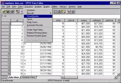
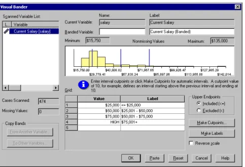
The Transform menu, as shown in Figure 1-1, provides options for case-level transformations, such as recoding data values and computing new data values (see Figure 1-2).
Figure 1-1
Figure 1-2
Recoding scale values into banded categories
This book does not discuss the graphical user interface in any great detail. The Help system provides detailed tutorials about using the graphical user interface, and almost all dialog boxes have Help buttons that display dialog-box-specific Help topics.
Command Language
The primary emphasis of this book is on using the SPSS command language, or command syntax, to write programs to solve data management problems. Although the command language may not be as user friendly as the graphical user interface, it has several distinct advantages:
You can save command files and run them repeatedly and in unattended batch mode.
Some data management facilities are available only through the command language and are not available via the menus and dialog boxes.
Command syntax provides documentation of your work, making it clear how you obtained your results and making it possible to reproduce them.
Macro Facility
SPSS has a macro facility that can be used to streamline the coding of repetitive commands and build command streams that can be run many times with varied parameters. You could, for example, create a complex command stream in which a variable or filename appears multiple times, define that stream as a macro with the name as an argument, and then call that stream as part of a job simply by naming the macro and specifying the name as an argument. Or, you could define a stream that iterates across a list of names. See Chapter 6 for more information about the macro facility.
Scripting Facility
In addition to the command language and the macro facility, you can automate many tasks with the SPSS scripting facility using standard programming languages, such as Visual Basic and C++.
Working with Command Syntax
If you haven’t worked with SPSS command syntax before, there are a few things you should know. A detailed introduction to SPSS command syntax is available in the “Universals” section in the SPSS Command Syntax Reference.
Creating Command Syntax Files
An SPSS command file is a simple text file. You can use any text editor to create a command syntax file, but SPSS provides a number of tools to make your job easier. Most features available in the graphical user interface have command syntax equivalents, and there are several ways to reveal this underlying command syntax:
Use the Paste button. Make selections from the menus and dialog boxes, and then click the Paste button instead of the OK button. This will paste the underlying commands into a command syntax window.
Record commands in the log. Select Display commands in the log on the Viewer tab in the Options dialog box (Edit menu, Options). As you run analyses, the
commands for your dialog box selections will be recorded and displayed in the log in the Viewer window. You can then copy and paste the commands from the Viewer into a syntax window or text editor.
Retrieve commands from the journal file. Most actions that you perform in the graphical user interface (and all commands that you run from a command syntax window) are automatically recorded in the journal file in the form of command syntax. The default name of the journal file is spss.jnl. The default location varies, depending on your operating system. Both the name and location of the journal file are displayed on the General tab in the Options dialog box (Edit menu, Options).
Running SPSS Commands
Once you have a set of commands, you can run the commands in a number of ways:
Highlight the commands that you want to run in a command syntax window and click the Run button.
Invoke one command file from another with the INCLUDE or INSERT command (see Chapter 2 for more information).
Use the Production Facility to create production jobs that can run unattended and even start unattended (and automatically) using common scheduling software. See the Help system for more information about the Production Facility.
Use SPSSB (available only with the server version) to run command files from a command line and automatically route results to different output destinations in different formats. See the SPSSB documentation supplied with the SPSS server software for more information.
Figure 1-3
Syntax Rules
Commands run from a command syntax window during a typical SPSS session must follow the interactive command syntax rules:
Each command must start on a new line.
Each command must end with a period (.).
Commands files run via SPSSB or the Production Facility or invoked via the INCLUDE
command must follow the batch command syntax rules:
Each command must start in the first column of a new line.
Each command continuation line must be indented at least one space.
The command terminator (a period) is optional.
If you adhere to the batch rules and also include a period at the end of each command, your command syntax will run in either mode. Command syntax pasted from dialog box selections is compatible with both interactive and batch modes.
CASE doesn’t MaTTeR (mostly)
For the most part, SPSS command syntax is not case sensitive.
Commands and keywords are not case sensitive. Examples in this book display command names and keywords in upper case simply to distinguish them from user-specified parameters.
Variable names can be defined with any mixture of upper- and lowercase characters, and case is preserved for display purposes.
Commands that refer to existing variable names are not case sensitive. For example, FREQUENCIES VARIABLES = newvar and frequencies variables = NEWVAR are functionally equivalent.
String values are case sensitive. This includes string data values and quoted strings. For example, the conditional statement IF (stringvar="abc") is false if the value of stringvar is “Abc”.
Using This Book
This book is intended for use with SPSS release 13.0 or later. Many examples will work with earlier versions, but some commands and features are not available in earlier releases.
Most of the examples shown in this book are designed as hands-on exercises that you can perform yourself. The CD that comes with the book contains the command files and data files used in the examples. All of the sample files are contained in the examples folder.
\examples\commands contains SPSS command syntax files.
\examples\data contains data files in a variety of formats.
\examples\scripts contains sample scripts.
All of the sample command files that contain file access commands assume that you have copied the examples folder to your C drive. For example:
GET FILE='c:\examples\data\duplicates.sav'.
SORT CASES BY ID_house(A) ID_person(A) int_date(A) . AGGREGATE OUTFILE = 'C:\temp\tempdata.sav'
Many examples, such as the one above, also assume that you have a c:\temp folder for writing temporary files. You can access command and data files from the
accompanying CD, substituting the drive location for c: in file access commands. For commands that write files, however, you need to specify a valid folder location on a device for which you have write access.
Documentation Resources
The SPSS Base User’s Guide documents the data management tools available through the graphical user interface. The material is similar to that available in the Help system. In addition to the chapters on “Data Files,” “Data Preparation,” “Data
Transformations,” and “File Handling and File Transformations,” see:
“Production Facility” for information about running unattended batch-mode SPSS jobs
The SPSS Command Syntax Reference, which is installed as a PDF file with the SPSS system, is a complete guide to the specifications for each SPSS command. The guide provides many examples illustrating individual commands. It has only a few extended examples illustrating how commands can be combined to accomplish the kinds of tasks that analysts frequently encounter. Sections of the SPSS Command Syntax Reference of particular interest include:
The DEFINE—!ENDDEFINE command, which covers the macro facility
The appendix “Using the Macro Facility,” which includes additional examples
The appendix “Defining Complex Files,” which covers the commands specifically intended for reading common types of complex files
The INPUT PROGRAM—END INPUT PROGRAM command, which provides rules for working with input programs
For additional information about scripting, see the SPSS for Windows Developer’s Guide, which is included on the SPSS installation CD in the SPSS\developer folder.
11
C h a p t e r
2
Best Practices and
Efficiency Tips
Introduction
If you haven’t worked with SPSS command syntax before, you will probably start with simple jobs that perform a few basic tasks. Since it is easier to develop good habits while working with small jobs than to try to change bad habits once you move to more complex situations, you may find the information in this chapter helpful.
Some of the practices suggested in this chapter are particularly useful for large projects involving thousands of lines of code, many data files, and production jobs run on a regular basis and/or on multiple data sources.
Customizing the Programming Environment
There are a few global settings and customization features that may make working with command syntax a little easier.
Displaying Commands in the Log
By default, commands that have been run are not displayed in the log, which can make it difficult to interpret error messages. To display commands in the log, use the command:
Or, using the graphical user interface:
E From the menus, choose:
Edit Options...
E Click the Viewer tab.
E Select (check) Display commands in the log. Figure 2-1
Log with and without commands displayed
Displaying the Status Bar in Command Syntax Windows
In addition to various status messages, the status bar at the bottom of a command syntax window displays the current line number and character position within the line. Since error messages typically contain information about the column position where an error was encountered, the column position information in the status bar can help you to pinpoint errors. (Note: You may have to increase the width of the command syntax window to see this information.)
The status bar is displayed by default. If it is currently not displayed, select Status Bar from the View menu in the command syntax window.
Figure 2-2
Status bar in command syntax window with current line number and column position displayed
Customizing the Toolbars
SPSS provides a simple drag-and-drop interface for creating customized toolbars that use buttons as shortcuts for virtually any menu item. You can also create custom buttons that run specific command syntax files or script files. To create customized toolbars:
E From the menus, choose:
View Toolbars...
E Select the window type for which you want to create or modify a toolbar. E Click Customize to modify an existing toolbar, or click New Toolbar to create a
completely new toolbar.
For detailed information about customizing toolbars, click the Help button in any of the toolbar customization dialog boxes.
Example
The following toolbar combines items from the File, Run, and Help menus, all added to the syntax window toolbar simply by dragging and dropping selections from list boxes to the toolbar. It also contains one custom toolbar button that runs a script. Figure 2-3
Customized toolbar
The first two buttons are shortcuts to the following menu selections:
File New Data and File New Syntax
Both selections are often useful when writing and debugging command syntax.
The next four buttons are shortcuts to the Run menu items that you can use to run different segments of a command syntax file: Current, Selection, To End, and All.
After the Run buttons, the next two buttons display the command syntax chart for the current command (your cursor location) and the PDF version of the detailed SPSS Command Syntax Reference, respectively. Clicking the latter button displays the first page of the guide, not the section for the current command; the icon shown has been edited to depict an open book rather than the default generic icon provided for “user-defined” items.
These two items may be a little hard to find when creating customized toolbars. The item for adding a button for context-sensitive syntax charts is Syntax Help in the Help category in the Customize Toolbar dialog box, and the item for adding a button for the SPSS Command Syntax Reference PDF is in the User-Defined category (although it is not actually “user-defined”).
The last button is a custom control that launches a customized script called CountNumberOfErrors.SBS, located in the examples\scripts folder. This script calculates and displays the number of errors encountered in a designated block of commands. For more information about this script, see “Count Number of Errors” on p. 274 in Chapter 7.
Additional Utility Scripts
The accompanying CD contains additional utility scripts that you may want to include as custom controls on your toolbar.
DeleteStatisticsAndCaseProcessingSummary.sbs. Deletes Statistics and Case
Processing tables from the Viewer. (As an alternative, you could use the OMS
command to simply prevent these table types from ever appearing in the Viewer, using the VIEWER=NO setting.)
EmptyDesignatedOutputWindow.sbs. Deletes all of the contents of the designated
Viewer window and displays the number of errors encountered so far in the session.
ExportViewerToSingleExcelSheet.sbs. Exports visible SPSS pivot tables, standard
charts, and interactive charts to Excel. Before executing this script, open a worksheet in Excel and select the cell/row in which pasting should start.
FindErrorMessages.sbs. Find error messages in logs and text blocks. Warnings objects
and items that are not visible are not included.
FindOutlineText.sbs. Searches for the specified text string in the outline pane of the
designated Viewer window. The search is not case sensitive.
ReplaceLeftPanePageTitle.sbs. Replaces “Page Title” in the outline pane with a
portion of the content of the page title. This is useful for placing quick references in the outline pane to locate given areas of the output. It has no effect if no page titles have been created. Page titles are different from the object titles that also appear in the outline. They are created by the TITLE command or, in the Viewer, by selecting Page Title from the Insert menu.
PrintSyntaxFile.sbs. Saves and prints the currently designated syntax window. The
filename, path, date, timestamp, and page numbers are printed
ConvertSyntaxToScript.sbs. Converts the command syntax of the designated syntax
window into the corresponding script format. The resulting command syntax is pasted at the end of the designated syntax window.
Protecting the Original Data
The original data file should be protected from modifications that may alter or delete original variables and/or cases. If the original data are in an external file format (for example, text, Excel, or database), there is little risk of accidentally overwriting the original data while working in SPSS. However, if the original data are in SPSS-format data files (.sav), there are many transformation commands that can modify or destroy the data, and it is not difficult to inadvertently overwrite the contents of an SPSS-format data file. Overwriting the original data file may result in a loss of data that cannot be retrieved.
There are several ways in which you can protect the original data, including:
Storing a copy in a separate location, such as on a CD, that can’t be overwritten.
Using the operating system facilities to change the read-write property of the file to read-only. If you aren’t familiar with how to do this in the operating system, you can use Mark File Read Only on the File menu or the new PERMISSIONS
subcommand on the SAVE command.
The ideal situation is then to load the original (protected) data file into SPSS and do all data transformations, recoding, and calculations using SPSS. The objective is to end up with one or more command syntax files that start from the original data and produce the required results without any manual intervention.
Do Not Overwrite Original Variables
It is often necessary to recode or modify original variables, and it is good practice to assign the modified values to new variables and keep the original variables unchanged. For one thing, this allows comparison of the initial and modified values to verify that the intended modifications were carried out correctly. The original values can subsequently be discarded if required.
Example
*These commands overwrite existing variables. COMPUTE var1=var1*2.
RECODE var2 (1 thru 5 = 1) (6 thru 10 = 2). *These commands create new variables. COMPUTE var1_new=var1*2.
RECODE var2 (1 thru 5 = 1) (6 thru 10 = 2)(ELSE=COPY) /INTO var2_new.
The difference between the two COMPUTE commands is simply the substitution of a new variable name on the left side of the equals sign.
The second RECODE command includes the INTO subcommand, which specifies a new variable to receive the recoded values of the original variable. ELSE=COPY
makes sure that any values not covered by the specified ranges are preserved.
Using Temporary Transformations
You can use the TEMPORARY command to temporarily transform existing variables for analysis. The temporary transformations remain in effect through the first command that reads the data (for example, a statistical procedure), after which the variables revert to their original values.
Example
*temporary.sps.
data list free /var1 var2. begin data 1 2 3 4 5 6 7 8 9 10 end data. TEMPORARY. COMPUTE var1=var1+5.
RECODE var2 (1 thru 5=1) (6 thru 10=2). FREQUENCIES
/VARIABLES=var1 var2
/STATISTICS=MEAN STDDEV MIN MAX. DESCRIPTIVES
/VARIABLES=var1 var2
/STATISTICS=MEAN STDDEV MIN MAX.
The transformed values from the two transformation commands that follow the
TEMPORARY command will be used in the FREQUENCIES procedure.
The original data values will be used in the subsequent DESCRIPTIVES procedure, yielding different results for the same summary statistics.
Under some circumstances, using TEMPORARY will improve the efficiency of a job when short-lived transformations are appropriate. Ordinarily, the results of
transformations are written to the virtual active file for later use and eventually are merged into the saved SPSS data file. However, temporary transformations will not be
written to disk, assuming that the command that concludes the temporary state is not otherwise doing this, saving both time and disk space. (TEMPORARY followed by
SAVE, for example, would write the transformations.)
If many temporary variables are created, not writing them to disk could be a noticeable saving with a large data file. However, some commands require two or more passes of the data. In this situation, the temporary transformations are recalculated for the second or later passes. If the transformations are lengthy and complex, the time required for repeated calculation might be greater than the time saved by not writing the results to disk. Experimentation may be required to determine which approach is more efficient.
Using Temporary Variables
For transformations that require intermediate variables, use scratch (temporary) variables for the intermediate values. Any variable name that begins with a pound sign (#) is treated as a scratch variable that is discarded at the end of the series of
transformation commands when SPSS encounters an EXECUTE command or other command that reads the data (such as a statistical procedure).
Example
*scratchvar.sps. DATA LIST FREE / var1. BEGIN DATA
1 2 3 4 5 END DATA.
COMPUTE factor=1.
LOOP #tempvar=1 TO var1.
- COMPUTE factor=factor * #tempvar. END LOOP.
Figure 2-4
Result of loop with scratch variable
The loop structure computes the factorial for each value of var1 and puts the factorial value in the variable factor.
The scratch variable #tempvar is used as an index variable for the loop structure.
For each case, the COMPUTE command is run iteratively up to the value of var1.
For each iteration, the current value of the variable factor is multiplied by the current loop iteration number stored in #tempvar.
The EXECUTE command runs the transformation commands, after which the scratch variable is discarded.
The use of scratch variables doesn’t technically “protect” the original data in any way, but it does prevent the data file from getting cluttered with extraneous variables. If you need to remove temporary variables that still exist after reading the data, you can use the DELETE VARIABLES command to eliminate them.
Using Command Syntax to Document Work
Contrary to what many new SPSS users generally expect, it is often almost as easy— and sometimes even easier—to create a command syntax file (which is a program) as it is to select menu and dialog box options. Command syntax also has a number of distinct advantages:
Documentation. The commands represent step-by-step documentation of how you obtained your results.
Verification. Anyone can easily rerun the command syntax and compare the results.
Reuse. You can automate common tasks performed on a routine basis.
Creating Command Syntax Files
If you’re new to SPSS command syntax, there are a number of tools to help you get started. Most features available in the graphical user interface have command syntax equivalents, and there are several ways to reveal that underlying command syntax:
Use the Paste button. Make selections from the menus and dialog boxes, and then click the Paste button instead of the OK button. This will paste the underlying commands into a command syntax window.
Record commands in the log. Select Display commands in the log on the Viewer tab in the Options dialog box (Edit menu, Options). As you run analyses, the
commands for your dialog box selections will be recorded and displayed in the log in the Viewer window. You can then copy and paste the commands from the Viewer to a syntax window or text editor. See “Displaying Commands in the Log” on p. 11 for more information.
Retrieve commands from the journal file. Most actions that you perform in the graphical user interface (and all commands that you run from a command syntax window) are automatically recorded in the journal file in the form of command syntax. The default name of the journal file is spss.jnl. The default location varies, depending on your operating system. Both the name and location of the journal file are displayed on the General tab in the Options dialog box (Edit menu, Options).
Use the script define_variables.sbs. Use this script (located in the examples\scripts folder) to generate variable definition command syntax based on the current properties of the working data file. If you use Variable View in the Data Editor to define variable properties, such as variable labels, value labels, and missing values, there is no Paste button and none of these actions will be recorded in the log or journal. This script generates the equivalent command syntax based on the defined properties of the variables in the working data file.
Use EXECUTE Sparingly
SPSS is designed to work with large data files (the current version can accommodate 2.15 billion cases). Since going through every case of a large data file takes time, the software is also designed to minimize the number of times it has to read the data. Statistical and charting procedures always read the data, but most transformation commands (for example, COMPUTE, RECODE, COUNT, SELECT IF) do not require a separate data pass.
The default behavior of the graphical user interface, however, is to read the data for each separate transformation so that you can see the results in the Data Editor immediately. Consequently, every transformation command generated from the dialog boxes is followed by an EXECUTE command. So, if you create command syntax by pasting from dialog boxes or copying from the log or journal, your command syntax may contain a large number of superfluous EXECUTE commands that can significantly increase the processing time for very large data files.
In most cases, you can remove virtually all of the auto-generated EXECUTE
commands, which will speed up processing, particularly for large data files and jobs that contain many transformation commands.
To turn off the automatic, immediate execution of transformations and the associated pasting of EXECUTE commands:
E From the menus, choose:
Edit Options...
E Click the Data tab.
E Select Calculate values before used.
Lag Functions
One notable exception to the above rule is transformation commands that contain lag functions. In a series of transformation commands without any intervening EXECUTE
commands or other commands that read the data, lag functions are calculated after all other transformations, regardless of command order. While this might not be a consideration most of the time, it requires special consideration in the following cases:
The lag variable is also used in any of the other transformation commands.
One of the transformations selects a subset of cases and deletes the unselected cases, such as SELECT IF or SAMPLE.
Example
*lagfunction.sps. *create some data. DATA LIST FREE /var1. BEGIN DATA
1 2 3 4 5 END DATA.
COMPUTE var2=var1.
********************************. *Lag without intervening EXECUTE. COMPUTE lagvar1=LAG(var1).
COMPUTE var1=var1*2. EXECUTE.
********************************. *Lag with intervening EXECUTE. COMPUTE lagvar2=LAG(var2). EXECUTE.
COMPUTE var2=var2*2. EXECUTE.
Figure 2-5
Results of lag functions displayed in Data Editor
Although var1 and var2 contain the same data values, lagvar1 and lagvar2 are very different from each other.
Without an intervening EXECUTE command, lagvar1 is based on the transformed values of var1.
With the EXECUTE command between the two transformation commands, the value of lagvar2 is based on the original value of var2.
Any command that reads the data will have the same effect as the EXECUTE
command. For example, you could substitute the FREQUENCIES command and achieve the same result.
In a similar fashion, if the set of transformations includes a command that selects a subset of cases and deletes unselected cases (for example, SELECT IF), lags will be computed after the case selection. You will probably want to avoid case selection criteria based on lag values—unless you EXECUTE the lags first.
Using $CASENUM to Select Cases
The value of the system variable $CASENUM is dynamic. If you change the sort order of cases, the value of $CASENUM for each case changes. If you delete the first case, the case that formerly had a value of 2 for this system variable now has the value 1. Using the value of $CASENUM with the SELECT IF command can be a little tricky because SELECT IF deletes each unselected case, changing the value of $CASENUM for all remaining cases.
For example, a SELECT IF command of the general form: SELECT IF ($CASENUM > [positive value]).
will delete all cases because, regardless of the value specified, the value of
$CASENUM for the current case will never be greater than 1. When the first case is evaluated, it has a value of 1 for $CASENUM and is therefore deleted because it doesn’t have a value greater than the specified positive value. The erstwhile second case then becomes the first case, with a value of 1, and is consequently also deleted, and so on.
The simple solution to this problem is to create a new variable equal to the original value of $CASENUM. However, command syntax of the form:
COMPUTE CaseNumber=$CASENUM.
SELECT IF (CaseNumber > [positive value]).
will still delete all cases because each case is deleted before the value of the new variable is computed. The correct solution is to insert an EXECUTE command between COMPUTE and SELECT IF, as in:
COMPUTE CaseNumber=$CASENUM. EXECUTE.
SELECT IF (CaseNumber > [positive value]).
MISSING VALUES Command
If you have a series of transformation commands (for example, COMPUTE, IF,
RECODE) followed by a MISSING VALUES command that involves the same variables, you may want to place an EXECUTE statement before the MISSING VALUES command. This is because the MISSING VALUES command changes the dictionary before the transformations take place.
Example
IF (x = 0) y = z*2. MISSING VALUES x (0).
The cases where x = 0 would be considered user missing on x, and the transformation of y would not occur. Placing an EXECUTE before MISSING VALUES allows the transformation to occur before 0 is assigned missing status.
WRITE and XSAVE Commands
In some circumstances, it may be necessary to have an EXECUTE command after a
WRITE or an XSAVE command. See “Using XSAVE in a Loop to Build a Data File” on p. 150 and “Using Command Syntax to Write Command Syntax” on p. 152 in Chapter 5 for more information.
Using Comments
It is always a good practice to include explanatory comments in your code. In SPSS, you can do this in several ways:
COMMENT Get summary stats for scale variables.
* An asterisk in the first column also identifies comments. FREQUENCIES
VARIABLES=income ed reside
/FORMAT=LIMIT(10) /*avoid long frequency tables /STATISTICS=MEAN /*arithmetic average*/ MEDIAN.
* A macro name like !mymacro in this comment may invoke the macro. /* A macro name like !mymacro in this comment will not invoke the
macro*/.
The first line of a comment can begin with the keyword COMMENT or with an asterisk (*).
Comment text can extend for multiple lines and can contain any characters. The rules for continuation lines are the same as for other commands. Be sure to terminate a comment with a period. See “Syntax Rules” on p. 7 in Chapter 1 for more information.
Use /* and */ to set off a comment within a command.
The closing */ is optional when the comment is at the end of the line. The command can continue onto the next line just as if the inserted comment was a blank.
To ensure that comments that refer to macros by name don’t accidently invoke those macros, use the /* [comment text] */ format.
Using SET SEED to Reproduce Random Samples or Values
When doing research involving random numbers—for example, when randomly assigning cases to experimental treatment groups—you should explicitly set the random number seed value if you want to be able to reproduce the same results.
The random number generator is used by the SAMPLE command to generate random samples and is used by many distribution functions (for example, NORMAL, UNIFORM) to generate distributions of random numbers. The generator begins with a seed, a large integer. Starting with the same seed, the system will repeatedly produce the same sequence of numbers and will select the same sample from a given data file. At the start of each session, the seed is set to a value that may vary or may be fixed, depending on your current settings. The seed value changes each time a series of transformations contains one or more commands that use the random number generator.
Example
To repeat the same random distribution within a session or in subsequent sessions, use
SET SEED before each series of transformations that use the random number generator to explicitly set the seed value to a constant value.
*set_seed.sps.
GET FILE = 'c:\examples\data\onevar.sav'. SET SEED = 123456789.
SAMPLE .1. LIST. SHOW SEED.
GET FILE = 'c:\examples\data\onevar.sav'. SET SEED = 123456789.
SAMPLE .1. LIST.
Before the first sample is taken the first time, the seed value is explicitly set with
SET SEED.
The LIST command causes the data to be read and the random number generator to be invoked once for each original case. The result is an updated seed value.
The second time the data file is opened, SET SEED sets the seed to the same value as before, resulting in the same sample of cases.
Both SET SEED commands are required because you aren’t likely to know what the initial seed value is unless you set it yourself.
Note: This example opens the data file before each SAMPLE command because successive SAMPLE commands are cumulative within the working data file.
Divide and Conquer
A time-proven method of winning the battle against programming bugs is to split the tasks into separate, manageable pieces. It is also easier to navigate around a syntax file of 200–300 lines than one of 2,000–3,000 lines.
Therefore, it is good practice to break down a program into separate stand-alone files, each performing a specific task or set of tasks. For example, you could create separate command syntax files to:
Prepare and standardize data.
Merge data files.
Perform tests on data.
Report results for different groups (for example, gender, age group, income category).
Using the INSERT command and a master command syntax file that specifies all of the other command files, you can partition all of these tasks into separate command files.
Using INSERT with a Master Command Syntax File
The INSERT command provides a method for linking multiple syntax files together, making it possible to reuse blocks of command syntax in different projects by using a “master” command syntax file that consists primarily of INSERT commands that refer to other command syntax files.
Example
INSERT FILE = "c:\examples\data\prepare data.sps" CD=YES. INSERT FILE = "combine data.sps".
INSERT FILE = "do tests.sps". INSERT FILE = "report groups.sps".
Each INSERT command specifies a file that contains SPSS command syntax.
By default, inserted files are read using interactive syntax rules, and each command should end with a period.
The first INSERT command includes the additional specification CD=YES. This changes the working directory to the directory included in the file specification, making it possible to use relative (or no) paths on the subsequent INSERT
INSERT versus INCLUDE
INSERT is a newer, more powerful and flexible alternative to INCLUDE. Files included with INCLUDE must always adhere to batch syntax rules, and command processing stops when the first error in an included file is encountered. You can effectively duplicate the INCLUDE behavior with SYNTAX=BATCH and ERROR=STOP on the
INSERT command.
Defining Global Settings
In addition to using INSERT to create modular master command syntax files, you can define global settings that will enable you to use those same command files for different reports and analyses.
Example
You can create a separate command syntax file that contains a set of FILE HANDLE
commands that define file locations and a set of macros that define global variables for client name, output language, and so on. When you need to change any settings, you change them once in the global definition file, leaving the bulk of the command syntax files unchanged.
*define_globals.sps.
FILE HANDLE data /NAME='c:\examples\data'.
FILE HANDLE commands /NAME='c:\examples\commands'. FILE HANDLE spssdir /NAME='c:\program files\spss'. FILE HANDLE tempdir /NAME='d:\temp'.
DEFINE !enddate()DATE.DMY(1,1,2004)!ENDDEFINE. DEFINE !olang()English!ENDDEFINE.
DEFINE !client()"ABC Inc"!ENDDEFINE. DEFINE !title()TITLE !client.!ENDDEFINE.
The first two FILE HANDLE commands define the paths for the data and command syntax files. You can then use these file handles instead of the full paths in any file specifications.
The third FILE HANDLE command contains the path to the SPSS folder. This path can be useful if you use any of the command syntax or script files that are installed with SPSS.
The last FILE HANDLE command contains the path of a temporary folder. It is very useful to define a temporary folder path and use it to save any intermediary files
created by the various command syntax files making up the project. The main purpose of this is to avoid crowding the data folders with useless files, some of which might be very large. Note that here the temporary folder resides on the D drive. When possible, it is more efficient to keep the temporary and main folders on different hard drives.
The DEFINE–!ENDDEFINE structures define a series of macros. This example uses simple string substitution macros, where the defined strings will be substituted wherever the macro names appear in subsequent commands during the session. See Chapter 6 for more information.
!enddate contains the end date of the period covered by the data file. This can be useful to calculate ages or other duration variables as well as to add footnotes to tables or graphs.
!olang specifies the output language.
!client contains the client’s name. This can be used in titles of tables or graphs.
!title specifies a TITLE command, using the value of the macro !client as the title text.
The master command syntax file might then look something like this:
INSERT FILE = "c:\examples\commands\define_globals.sps". !title.
INSERT FILE = "data\prepare data.sps". INSERT FILE = "commands\combine data.sps". INSERT FILE = "commands\do tests.sps". INCLUDE FILE = "commands\report groups.sps".
The first INCLUDE runs the command syntax file that defines all of the global settings. This needs to be run before any commands that invoke the macros defined in that file.
!title will print the client’s name at the top of each page of output.
"data" and "commands" in the remaining INSERT commands will be expanded to
"c:\examples\data" and "c:\examples\commands", respectively.
Note: Using absolute paths or file handles that represent those paths is the most reliable way to make sure that SPSS finds the necessary files. Relative paths may not work as you might expect, since they refer to the current working directory, which can change frequently. You can also use the CD command or the CD keyword on the INSERT
Global Subroutines
You can create much more sophisticated macros than these simple string substitution macros, including macros that take arguments that you specify in the macro calls. As a general rule, you may find it most useful to keep most macros in separate files, distinct from your regular command syntax files. You can then use the macro files as a library of global subroutines.
Example
This macro executes one set of commands for a list of categorical variables that you supply and another set of commands for a list of scale variables that you supply. This might be useful if you routinely generate the same descriptive and summary statistics as a preliminary step before further analysis, where the only thing that differs is the variables used in the summaries.
*macro_lib1.sps.
DEFINE !sumstat (catvars = !CHAREND('/') /scalevars = !CMDEND)
!IF (!catvars ~=!NULL) !THEN frequencies variables = !catvars /barchart.
!IFEND
!IF (!scalevars ~= !NULL) !THEN frequencies variables = !scalevars /format = notable
/statistics = mean median min max /histogram.
!IFEND !ENDDEFINE.
The macro contains two arguments: one for handling categorical variables and one for handling scale variables.
catvars = !CHAREND('/') specifies that any text in the macro call between catvars =
and the next forward slash encountered in the macro call will be used wherever
!catvars appears in the macro.
scalevars = !CMDEND specifies that any text in the macro call that appears after
scalevars = will be used wherever !scalevars appears in the macro.
Two FREQUENCIES commands are defined in the macro: one to use for categorical variables and one to use for scale variables.
The !IF statements make sure that the macro call includes a list of catvars and/or scalevars before running the respective FREQUENCIES command. This provides more flexibility, since the macro call can then contain one list of either kind or both lists without generating any errors.
You could then invoke the macro in several ways:
***First run the file that defines the macro***. INCLUDE FILE="c:\examples\commands\macro_lib1.sps".
***now run the macro with both catvars and scalevars***. !sumstat catvars = marital gender jobcat
/scalevars = income age edyears.
***now run it with just catvars***.
!sumstat catvars = marital gender jobcat. ***and now just scalevars***.
!sumstat scalevars = income age edyears.
The first macro call would generate two FREQUENCIES commands; the other two would each generate one FREQUENCIES command. In each case, the variables listed in the macro call would be used in the VARIABLES subcommand. Macros are discussed in greater detail in Chapter 6.
33
C h a p t e r
3
Getting Data into SPSS
Before you can work with data in SPSS, you need some data to work with. There are several ways to get data into the application:
Open a data file that has already been saved in SPSS format.
Enter data manually in the Data Editor.
Read a data file from another source, such as a database, text data file, spreadsheet, or SAS.
Opening an SPSS-format data file is simple, and manually entering data in the Data Editor is not likely to be your first choice, particularly if you have a large amount of data. This chapter focuses on how to read data files created and saved in other applications and formats.
Getting Data from Databases
SPSS relies on ODBC (open database connectivity) to read data from databases. ODBC is an open standard with versions available on many platforms, including Windows, UNIX, and Macintosh.
Installing Database Drivers
You can read data from any database format for which you have a database driver. In local analysis mode, the necessary drivers must be installed on your local computer. In distributed analysis mode (available with the server version), the drivers must be installed on the remote server.
ODBC database drivers for a wide variety of database formats are included on the SPSS installation CD, including: Access Btrieve DB2 dBASE Excel FoxPro Informix Oracle Paradox Progress SQL Base SQL Server Sybase
Most of these drivers can be installed by installing the SPSS Data Access Pack. You can install the SPSS Data Access Pack from the Autoplay menu on the SPSS installation CD.
If you need a Microsoft Access driver, you will need to install the Microsoft Data Access Pack. An installable version is located in the Microsoft Data Access Pack folder on the SPSS installation CD.
Before you can use the installed database drivers, you may also need to configure the drivers using the Windows ODBC Data Source Administrator. For the SPSS Data Access Pack, installation instructions and information on configuring data sources are located in the Installation Instructions folder on the SPSS installation CD.
Database Wizard
It’s probably a good idea to use the Database Wizard (File menu, Open Database) the first time you retrieve data from a database source. At the last step of the wizard, you can paste the equivalent commands into a command syntax window. Although the SQL generated by the wizard tends to be overly verbose, it also generates the CONNECT
Reading a Single Database Table
SPSS reads data from databases by reading database tables. You can read information from a single table or merge data from multiple tables in the same database. A single database table has basically the same two-dimensional structure as an SPSS data file: records are cases and fields are variables. So reading a single table can be very simple.
Example
This example reads a single table from an Access database. It reads all records and fields in the table.
*access1.sps.
GET DATA /TYPE=ODBC /CONNECT=
'DSN=MS Access Database;DBQ=C:\examples\data\dm_demo.mdb;'+ 'DriverId=25;FIL=MS Access;MaxBufferSize=2048;PageTimeout=5;' /SQL = 'SELECT * FROM CombinedTable'.
EXECUTE.
The GET DATA command is used to read the database.
TYPE=ODBC indicates that an ODBC driver will be used to read the data. This is required for reading data from any database, and it can also be used for other data sources with ODBC drivers, such as Excel workbooks (see “Reading Multiple Worksheets” on p. 43).
CONNECT identifies the data source. For this example, the CONNECT string was copied from the command syntax generated by the Database Wizard. The entire string must be enclosed in single or double quotes. In this example, we have split the long string onto two lines using a plus sign (+) to combine the two strings.
The SQL subcommand can contain any SQL statements supported by the database format. Each line must be enclosed in single or double quotes.
SELECT * FROM CombinedTable reads all of the fields (columns) and all records (rows) from the table named CombinedTable in the database.
Any field names that are not valid SPSS variable names are automatically converted to valid variable names, and the original field names are used as variable labels. In this database table, many of the field names contain spaces, which are removed in the variable names.
Figure 3-1
Database field names converted to valid variable names
Example
Now we’ll read the same database table—except this time, we’ll read only a subset of fields and records.
*access2.sps.
GET DATA /TYPE=ODBC /CONNECT=
'DSN=MS Access Database;DBQ=C:\examples\data\dm_demo.mdb;'+ 'DriverId=25;FIL=MS Access;MaxBufferSize=2048;PageTimeout=5;' /SQL =
'SELECT Age, Education, [Income Category]' ' FROM CombinedTable'
' WHERE ([Marital Status] <> 1 AND Internet = 1 )'. EXECUTE.
The SELECT clause explicitly specifies only three fields from the file; so the working data file will contain only three variables.
The WHERE clause will select only records where the value of the Marital Status field is not 1 and the value of the Internet field is 1. In this example, that means only unmarried people who have Internet service will be included.
Two additional details in this example are worth noting:
The field names Income Category and Marital Status are enclosed in brackets. Since these field names contain spaces, they must be enclosed in brackets or quotes. Since single quotes are already being used to enclose each line of the SQL statement, the alternative to brackets here would be double quotes.
We’ve put the FROM and WHERE clauses on separate lines to make the code easier to read; however, in order for this command to be read properly, each of those lines also has a blank space between the starting single quote and the first word on the line. When the command is processed, all of the lines of the SQL statement are merged together in a very literal fashion. Without the space before WHERE, the program would attempt to read a table named CombinedTableWhere, and an error would result. As a general rule, you should probably insert a blank space between the quotation mark and the first word of each continuation line.
Reading Multiple Tables
You can combine data from two or more database tables by “joining” the tables. The working data file can be constructed from more than two tables, but each “join” defines a relationship between only two of those tables:
Inner join. Records in the two tables with matching values for one or more specified fields are included. For example, a unique ID value may be used in each table, and records with matching ID values are combined. Any records without matching identifier values in the other table are omitted.
Left outer join. All records from the first table are included regardless of the criteria used to match records.
Right outer join. Essentially the opposite of a left outer join. So the appropriate one to use is basically a matter of the order in which the tables are specified in the SQL
SELECT clause. Example
In the previous two examples, all of the data resided in a single database table. But what if the data were divided between two tables? This example merges data from two