Numerical and experimental study of the flow around
a 4:1 rectangular cylinder at moderate Reynolds number
Amandine Guissart∗, Thomas Andrianne, Greg Dimitriadis, Vincent E. Terrapon
Department of Aerospace and Mechanical Engineering, University of Li`ege, All´ee de la D´ecouverte 9, 4000 Li`ege, Belgium
Abstract
This paper presents the results of investigations into the flow around a rectangular cylinder with a chord-to-depth ratio equal to 4. The studies are performed through wind tunnel dynamic pressure measurements along a cross-section combined with Unsteady Reynolds-Averaged Navier-Stokes (urans) and Delayed-Detached Eddy Simulation (ddes). These experimental and numerical
studies are complementary and combining them allows a better understanding of the unsteady dynamics of the flow. The comparison of experimental and numerical data is performed using statistics and Dynamic Mode Decomposition. It is shown that the rectangular cylinder involves complex separation-reattachment phenomena that are highly sensitive to the Reynolds number. In particular, the mean lift slopeclαincreases rapidly with the Reynolds number in the range 7.8×10³ ≤Re≤1.9×10⁴due to the modification of the mean vortex strength, thickness and distance from the surface. Additionally, it is shown that bothuransandddessimulations fail to accurately predict the flow at all the different incidence angles considered. Theuransapproach is able to qualitatively estimate the spatio-temporal variations of vortices for incidences below the stall angleα=4◦. Nonetheless,
uransdoes not predict stall, while ddescorrectly identifies the stall angle observed experimentally.
Keywords: bluffbody, rectangular cylinder,urans,ddes, unsteady pressure measurements, aerodynamics. 1. Introduction
1
Despite the simple two-dimensional geometries involved, the 2
flow around bodies of elongated rectangular cross section are 3
highly complex because of the three-dimensional nature of tur-4
bulence and the unsteady separation and reattachment dynamics 5
characterizing bluffbodies. Rectangular cylinders at zero inci-6
dence have been extensively studied, first experimentally (e.g. 7
Nakaguchi et al.,1968;Nakamura and Mizota,1975;Washizu
8
et al.,1978;Okajima,1983;Stokes and Welsh,1986) and then 9
numerically (e.g. Tamura et al.,1993;Yu and Kareem,1998; 10
Shimada and Ishihara,2002). These authors have shown that 11
the flow dynamics around such cross sections is mainly influ-12
enced by the ratio of the chord c to the dephd of the cross 13
section. In particular,Shimada and Ishihara(2002) investigated 14
the impact of thec/d ratio at zero incidence through Unsteady
15
Reynolds-Average Navier-Stokes (urans) simulations at Re = 16
2.2×10⁴, this Reynolds number being defined as Re = U∞d/ν, 17
whereU∞andνare the freestream velocity and the kinematic
18
viscosity, repectively.Shimada and Ishihara(2002) divided the 19
aerodynamic behavior into three main categories based on the 20
dynamics of the shear layer. For short cylinders withc/d≤2.8,
21
flow separation occurs at the leading edges and the rectangular 22
cross section is too short to allow shear layer reattachment. The 23
flow is thus fully separated and vortices are periodically shed 24
from the leading edges of the cylinder. On rectangular cross 25
∗
Corresponding author
Email address:[email protected](Amandine Guissart)
sections with a ratio 2.8 < c/d < 6, the shear layer reattaches
26
periodically and vortex shedding occurs from both the leading 27
and trailing edges. Finally, for longer rectangular cylinders with 28
c/d ≥6 , the flow is able to fully reattach and vortices are shed
29
from the trailing edges. 30
In this context, the Benchmark on the Aerodynamics of a 31
Rectangular Cylinder (barc) (Bartoli et al.,2008) provides ex-32
perimental and numerical contributions to the study of a 5:1 33
rectangular cylinder. Bruno et al.(2014) compared more than 34
70 studies in terms of bulk parameters, flow and pressure statis-35
tics, as well as spanwise correlations. Among the principal con-36
clusions,Bruno et al.(2014) reported a narrow distribution of 37
results obtained for the Strouhal number and the mean drag co-38
efficient while those collected for the standard deviation of the 39
lift coefficient are significantly dispersed. It was argued that this 40
scattering is caused by the high sensitivity of the flow along the 41
upper and lower surfaces of the rectangular cylinder to small 42
differences in the wind tunnel setup and in the simulation pa-43
rameters. Within the framework of the barc, Schewe (2013) 44
investigated experimentally the impact of Reynolds number in 45
the range between 4×10³and 4×10⁵on the aerodynamic co-46
efficients. He showed that the Reynolds number has a minor 47
influence on both the drag coefficient and the Strouhal number, 48
but significantly impacts the lift coefficient and particularly the 49
lift curve slope. Schewe(2013) argued that an increase in the 50
Reynolds number could correspond to an increase in the turbu-51
lence level which would cause a shift downstream of the mean 52
reattachment point on the lower surface (for a cylinder at pos-53
itive angle of attack). This would lead to a modification of the 54
flow topology that could impact the pressure coefficient distri-55
bution and therefore the lift. The need for the wind engineer-56
ing community to capture accurately the slope of the lift coef-57
ficient is obvious: it appears (i) in the calculation of the critical 58
wind speed in the quasi-steady theory of galloping and (ii) in 59
the calculation of the buffeting response of structures subject to 60
turbulent wind flows. More recently,Patruno et al.(2016) per-61
formeduransand Large Eddy Simulations (les) at three angles 62
of attack. They reported large discrepancies betweenuransand 63
lesresults for the different incidences. Moreover, they showed 64
thaturansis not able to correctly estimate the internal organi-65
zation of the recirculation bubble, which impacts the estimation 66
of the spatio-temporal pressure coefficient and subsequently the 67
load coefficients. Finally,Mannini et al. (2017) used pressure 68
and load measurements to investigate the effects of the inci-69
dence, Reynolds number and turbulent intensity on the flow and 70
the subsequent bulk parameters. In particular, the Reynolds-71
number dependence of force coefficients and the effect of the 72
incoming turbulence on the vortex-shedding mechanism were 73
highlighted. 74
As an extension of the studies performed by Patruno et al.
75
(2016) andMannini et al.(2017), the present work investigates 76
both experimentally and numerically the flow around a rect-77
angular cylinder of aspect ratio c/d = 4, i.e., slightly shorter
78
that in the context of the barc but exhibiting similar dynam-79
ics. The spatio-temporal pressure distribution along a cross sec-80
tion of the cylinder is acquired by carrying out unsteady pres-81
sure measurements at different incidences and for 7.8×10³ < 82
Re<1.9×10⁴. The flow is also investigated through Compu-83
tational Fluid Dynamics (cfd) using bothurans and Delayed-84
Detached Eddy Simulation (ddes) approaches. The objective of 85
the present study is two-fold: i) to determine the effects of the 86
rectangle incidence and freestream velocity on the variation of 87
the flow topology and the aerodynamic loads, and ii) to assess 88
the capability of urans andddesto provide a sufficiently ac-89
curate estimation of the flow and the subsequent aerodynamic 90
loads for different incidences. 91
2. Methodology 92
Sections2.1and2.2are dedicated to the description of the 93
experiments and the setup of thecfdsimulations, respectively. 94
An extensive description of the experimental set-up can be 95
found inGuissart(2017). 96
2.1. Experimental approach 97
The measurements are conducted in a G¨ottingen-type wind 98
tunnel whose freestream turbulence intensity is below 2%. The 99
test section is 5 m long, 2.5 m wide and 1.8 m high. The main 100
Reynolds number studied in the following is Re = 1.1×10⁴, 101
which is based on a freestream velocityU∞ = 8.3 m/s. Four
102
additional freestream velocities are also considered to study the 103
impact of the Reynolds number in the range between 7.8×10³ 104
and 1.9×10⁴. These velocities are U
∞ = 6 m/s, 10.6 m/s,
105
12.8 m/s and 15 m/s. 106
The model consists of a hollow rectangular aluminum tube 107
of 2 mm thickness and 1 m length. Its cross-section is 8 cm ×
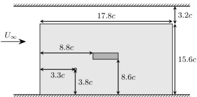
108 U∞ 17.8c 15.6c 3.2c 8.6c 8.8c 3.8c 3.3c
Figure 1: Schematic side view of the mounting apparatus where the rectangular cylinder is depicted in dark gray, the wooden plate in light gray, and the small disk represents the point where the reference freestream velocity and static pres-sure are meapres-sured.
2 cm, which corresponds to a chord-to-depth ratioc/d =4. The
109
cross-section edges are not perfectly sharp and their radiusrc 110
is such thatrc/d = 1.5%. The tube is attached horizontally on 111
one of its sides with ball bearings on a vertical beam. This 112
assembly leads to a single degree of freedom in pitch that is 113
clamped once the desired incidence is imposed. The other side 114
of the tube is located at a distance of 0.4cfrom the wind tunnel 115
wall to reduce three-dimensional effects. A wooden plate of 116
dimensions 15.6c×17.8cis added next to the vertical beam to 117
reduce as much as possible the impact of the mounting on the 118
flow around the rectangular cylinder. As depicted in Fig.1, the 119
rectangular tube is located relatively far from the edges of the 120
wooden plate and the boundary effects are thus assumed to be 121
small. 122
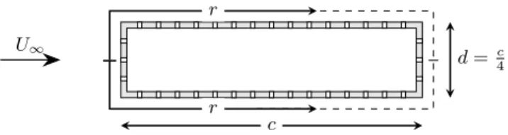
The pressure is sampled at several pressure taps located on a 123
cross-section of the rectangular cylinder as depicted in Fig.2. 124
This section located at the mid-span of the cylinder is cov-125
ered with 36 taps separated by a nominal distance of 5 mm 126
or 6.25% of the chord. Note that after the pressure taps were 127
drilled manually, their exact location is measured to an accu-128
racy of 0.2 mm. In the following, the taps are identified by their 129
non-dimensional curvilinear abscissar = r/c,r being defined
130
in Fig.2. Pressure is measured with a multi-channel Dynamic 131
PressureMeasurement System made by TFI and working in 132
the range±10 hPa to±35 hPa. This transducer measuresp−p∞,
133
the difference between the pressure pat a tap and a reference 134
pressure p∞ measured at the reference point shown in Fig.1.
135
The pressure taps are connected to the pressure transducer by 136
TransContinentalManufacturingtubes that are 1.34 m long 137
and have a documented internal diameter of 1.32 mm. Each 138
tube forms a pneumatic line that acts as a filter and causes 139
amplitude and phase distortions of the unsteady pressure sig-140
nal to be measured. Therefore, a correction is applied as a 141
post-processing step to retrieve the local unsteady pressure at 142
each tap. In particular, the theoretical correction proposed by 143
Bergh and Tijdeman(1965) is chosen. The freestream veloc-144
ity and static pressure being known, the pressure coefficient 145
Cp= p−p∞
1/2ρ
∞U∞ at each tap location can then be straightforwardly
146
computed. The pressure distribution is acquired for angles of 147
attack ranging from−7◦ to 8◦, the incidence angle being set
148
with an accuracy of 0.2◦. The sampling frequency fs is set to
149
500 Hz and each set of experiments lasts for 60 s. Assuming 150
U∞ d=c 4 c r r
Figure 2: Schematic sectional view of the pressure taps located on the rectangu-lar cylinder and definition of the coordinateralong the cylinder cross-section surface.
the Strouhal number St = f d/U
∞ = 0.13 (Washizu et al.,1978) 151
where f is the shedding frequency of the rectangular cylinder, 152
this sampling frequency corresponds to at least 5f and each set 153
contains more than 2 000 shedding cycles. 154
The pressure coefficient is first computed from the raw data 155
and filtered using a Butterworth 12thorder band-pass filter with 156
a frequency band from 10 to 200 Hz. Then, the amplitude and 157
phase distortions caused by the tube lines on the time response 158
ofCpare corrected by applying the method proposed byBergh 159
and Tijdeman(1965). Note that the sensitivity of the corrected 160
pressure to the input parameters required by this method has 161
been studied, and it has been demonstrated that the conclu-162
sions exposed below are robust to uncertainties associated with 163
them (Guissart,2017). Aerodynamic loads applied on the rect-164
angle are calculated by integrating the Cp distribution along 165
the rectangle surfaces. The integration is performed using the 166
trapezoidal rule. This leads to the two-dimensional sectional 167
coefficients of liftcl, dragcdand pitching momentcm, the latter 168
being computed about the cross section center and defined pos-169
itive nose-up. These three load coefficients are computed based 170
on the chord lengthc. Finally, the Strouhal number is computed 171
through Fourier analysis performed on the lift coefficient. 172
2.2. Computational approaches 173
Twocfdsimulation tools are used to compute the flow and 174
aerodynamic loads on the 4:1 cylinder: urans andddes. The 175
simulations are performed in OpenFOAM®. The implementa-176
tion characteristics of each model are presented below. 177
2.2.1. uranssimulations 178
The chosenuransmodel is thek−ωsstproposed byMenter 179
and Esch(2001) and modified byMenter et al.(2003). A tran-180
sient solver for incompressible flow based on the pimple al-181
gorithm is used with a non-dimensional time step ∆tU∞/cset to 182
10−3, i.e.,1/1700thof a typical shedding cycle. The second order
183
implicit backward Euler scheme is used to advance the equa-184
tions in time and second order schemes are chosen for spatial 185
discretization. In particular, the velocity gradient ∂iuj is dis-186
cretized through a second order, upwind-biased scheme. 187
As depicted in Fig.3, the computational domain is a square 188
of dimensions 50c×50ccentered vertically on the centroid of 189
the rectangular cylinder. The upstream and downstream borders 190
of this square are respectively distant of 19.5cand 30.5cfrom 191
the rectangle center. These dimensions are similar to those used 192
in most of the numerical studies performed in the context of the 193
barc(Bruno et al.,2014). The mesh is divided into an unstruc-194
tured and a structured parts. The structured region consists of 195 50c 50c 19.5c 30.5c 15d x y
Figure 3: Computational domain used for theuransandddessimulations.
a disc of radius 15dcentered on the rectangle and the zone of 196
the wake located downstream of the body. The simulations are 197
wall-resolved and the first mesh point away from the surface is 198
set such thaty+ ≈0.7 for most of the cells around the
rectan-199
gle. The grid consists of 140 cells spread along the chord of the 200
rectangular cylinder, 130 along its depth, 100 cells along the 201
radius of the circle surrounding the rectangle and 90 cells dis-202
cretizing horizontally the wake. It contains 75 000 hexahedra 203
and the grid independence of the results was verified through a 204
mesh convergence study. 205
At walls, the no-slip boundary condition is imposed for the 206
velocity and a zero-gradient condition is set for the pressure. 207
Dirichlet conditions are imposed for the turbulent scalars using 208
the automatic near-wall treatment proposed byMenter and Esch
209
(2001). At the inlet, the freestream velocity is imposed and the 210
pressure gradient is set to zero. The value of the turbulent ki-211
netic energyk∞is based on an inlet freestream turbulence
in-212
tensity of 0.3% and the specific dissipation rateω∞is such that
213
the turbulent eddy viscosity verifiesνt=5×10⁻³ν(Menter and 214
Esch,2001). The outlet corresponds to a zero-gradient for the 215
velocity and turbulent scalars, while the pressure is enforced. 216
Finally, a slip boundary condition is imposed for all variables at 217
the upper and lower boundaries of the domain, allowing only a 218
streamwise variation. 219
2.2.2. ddessimulations 220
The ddessimulations carried out within the context of the 221
present work are based on the original formulation of the 222
Spalart-Allmaras model (Spalart et al.,1997). The setup is very 223
similar to that ofurans, except for a few particular points spe-224
cific toddes. 225
As foruranssimulations, the transient incompressible solver 226
pimpleis selected. For stability purposes, the non-dimensional 227
time-step is decreased compared to theuranscases and set to 228
6.25×10⁻⁴. Similarly to the
urans setup, a backward Euler 229
scheme is chosen for temporal discretization. The same second-230
order schemes are also used for spatial discretization, except for 231
the non-linear advective term, which is discretized with a Lin-232
ear Upwind Stabilized Transport (lust) scheme, as suggested 233
byPatruno et al.(2016). 234
The two-dimensional computational domain depicted in 235
Fig. 3 is extruded along the z-direction to obtain a spanwise 236
length s = c. This dimension has been used in les studies 237
performed on similar cases (e.g.Yu and Kareem,1998;Bruno
238
et al., 2010) and verifies the criterion s/
c ≥ 1 suggested by
239
Tamura et al.(1998). Note however thatMannini et al.(2011) 240
showed that this common choice for the span is not enough 241
to allow the free development of large-scale turbulent struc-242
tures, which could lead to an overestimation of the load coeffi -243
cients’ second order statistics.Spalart and Streett(2001) argued 244
that the geometry-dependent turbulence structures are gener-245
ated in the “focus region” and that the maximum grid spacing 246
∆0within that region is the principal measure of the spatial res-247
olution inddes. This region is assumed here to extend up to half 248
a chord downstream of the rectangular cylinder’s trailing edges 249
and theddesmesh is designed to obtain∆0 =c/64, similarly to
250
Mannini et al. (2011) who demonstrated the strong impact of 251
this parameter on the results. The spanwise discretization is 252
∆z=c/
64and the grid in thex−yplane has to be modified
com-253
pared touransgrid to keep the extent of the “focus region”. In 254
particular, the chord and the depth of the rectangular cylinder 255
are divided into 200 and 130 cells, respectively, while 110 cells 256
are spread into the wake. Finally, a mesh made of 8.2 M cells is 257
obtained. 258
The boundary conditions for pressure and velocity are the 259
same as the ones described forurans. As a smooth freestream 260
flow is assumed, a Dirichlet boundary condition ˜ν = 0 is im-261
posed at the inlet while a Neumann condition is set for the out-262
let. A slip condition is imposed on the upper and lower bound-263
aries. Finally, periodic boundary conditions are adopted on the 264
two boundaries normal to the extrusion direction. 265
The ddesresults presented below are based on a computed 266
time window containing 150 non-dimensional time instances, 267
i.e., roughly 80 shedding cycles. A convergence study showed 268
that the mean and standard deviation of the aerodynamic coeffi -269
cients converged to within 5% after 150 time instances. More-270
over, the first 100 of the total 250 non-dimensional time units 271
contained in each ddessimulation were discarded in order to 272
eliminate the transient response. 273
2.3. Comparison of the different approaches 274
The experimental (exp) and numerical results are compared 275
through usual statistical analysis and via a spatio-temporal 276
decomposition technique (Dynamic Mode Decomposition, or 277
dmd). 278
First and second order statistics are computed on the time 279
response of the pressure and aerodynamic load coefficients. 280
The time-averaged values and the corresponding standard de-281
viations are respectively denoted by·and·0. The pressure
dis-282
tribution of interest corresponds toCp along the cross-section 283
of the rectangular cylinder. The three-dimensional pressure 284
distributions calculated by theddessimulations are first aver-285
aged along thez-direction. Note that the second order statistics 286
resulting from this averaging step are small, which is proba-287
bly due to the short span length that does not allow the devel-288
opment of large-scale structures (Mannini et al.,2011). First 289
and second order statistics are then computed on the resulting 290
hCpddes(x,t)i
z. Finally, becauseexpanduransresults are two-291
dimensional, the corresponding statistics are computed without 292
this span-averaging step. 293
The spatio-temporalexpandcfdresults are compared using 294
dmd, a technique proposed bySchmid(2010) that decomposes 295
data into single frequency modesφdmd
k describing the dynamic 296
process. The dynamical flow features are extracted from a tem-297
poral sequence ofNsnapshotsvnequidistant in time, each snap-298
shot being a column vector ofMtwo or three-dimensional spa-299
tial data. In particular, the M×N matrix of snapshotsVN1 = 300
{v1,v2, . . . ,vN}is decomposed into the variable-separated finite 301 sum 302 VN1 (x,t)= K X k=1 qdmd k φdmdk exp λdmd k t , (1) 303 where, φdmd k is thek
th spatial mode. The time response is ex-304 pressed asqdmd k exp λdmd k t , whereqdmdandλdmd k are respectively 305
the complex amplitude and frequency associated with the kth 306
mode, while tis the line vector containing the N time-steps. 307
In the present work,V1N consists of both the time response of 308
the load coefficients and the Cp distribution, Cp being span-309
averaged in the context ofddesresults. dmdis then used to re-310
construct an approximation of the results. To this end, the most 311
relevant modesφdmd
k are selected by descending order of am-312
plitudeqdmd
k and the approximated matrixbV N 1 is then calculated 313 from 314 b VN1 = X kthselected mode qdmd k φdmdk exp =λdmd k t. (2) 315
The number of selected modesφdmd
k is chosen to obtain statis-316
tics computed onbV1Nsimilar to those computed onVN1. In the
317
following, these modes correspond to the mean mode and the 318
modeφdmd
k associated with the shedding frequency. 319
3. Results 320
This section presents and discusses the results obtained ex-321
perimentally and numerically. Statistics computed on load and 322
pressure coefficients are discussed and compared in Secs.3.1
323
and3.2, respectively. Section3.3aims to understand the dy-324
namics of the flow by analysing the time response of the pres-325
sure distribution. Finally, Sec. 3.4 studies the effects of the 326
Reynolds number on the flow and the subsequent aerodynamic 327
loads. 328
3.1. Statistics on the load coefficients and Strouhal number 329
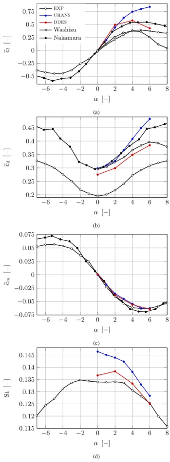
Figure4shows the aerodynamic coefficients and the Strouhal 330
number as a function of the incidence αat Re = 1.1 ×10⁴. 331
Experimental results reported byNakamura and Mizota(1975) 332
and Washizu et al.(1978) are also depicted for comparison. 333
Note that these authors specified only a range of Reynolds num-334
bers, which are respectively 104≤Re≤105and 2×10⁴ ≤Re≤ 335
3.3×10⁵, and not a precise value. 336
Figure4aplots the mean lift coefficient as a function of the 337
angle of attack. In particular,clexpclearly exhibits a linear in-338
crease withαfrom−4◦ to 4◦. In this linear region, the slope 339
clexp
α is approximately 2.1π. For |α| > 5◦, the absolute mean 340
lift coefficient decreases and the rectangular cylinder is stalled. 341
The mean drag coefficient is depicted in Fig. 4b. The varia-342
tion ofcdexpexhibits a classical parabolic variation for absolute 343
angles lower than 4◦. For higher incidence, as the rectangular
344
cylinder is stalled (decrease of lift), the increase in drag satu-345
rates. Finally, as shown in Fig. 4c, the variation of the mean 346
pitching moment about the center of the rectangular cylinder 347
exhibits a linear decrease for incidence |α| ≤ 2◦. The
corre-348
sponding slope iscmexp
α ≈ −0.35π. This linear behavior is fol-349
lowed by a saturation. For|α|>5◦, the absolutecmexpdecreases 350
slightly again. Finally, the Strouhal number is shown in Fig.4d. 351
For−3◦ < α <3◦, Stexpis nearly constant and equal to 0.134. 352
Then, for increasing incidence, Stexpdecreases linearly to reach 353
Stexp=0.116 forα=8◦.
354
The mean aerodynamic coefficients are compared to exper-355
imental results available in the literature. The slope clexp α is 356
relatively close to the value reported by Washizu et al.(1978) 357
(clα=2.3π) but very different from the result ofNakamura and
358
Mizota(1975) (clα =3.3π). As mentioned in Sec.1and later 359
illustrated in Sec.3.4, the mean lift slope can be very sensitive 360
to the Reynolds number. However, as the Reynolds number 361
associated with these works from the literature is not known 362
precisely, no conclusion can be drawn. The stall angle is sim-363
ilar for the three sets of results. However, the post-stall de-364
crease inclis higher for the results presented byNakamura and
365
Mizota(1975) and even higher for the experiments carried out 366
byWashizu et al.(1978). The mean dragcd at zero incidence 367
is identical for the two studies from the literature. However, 368
this value is higher by 0.1 compared to cdexp. For incidences 369
|α| < 4◦, the parabolic shape exhibited by the curve cdexp is 370
similar to the one obtained byWashizu et al.(1978), but the re-371
sults reported byNakamura and Mizota(1975) show a stronger 372
increase of the drag with the incidence. Some of those dis-373
crepancies can be explained by the difference in the load acqui-374
sition process, as Nakamura and Mizota (1975) andWashizu
375
et al.(1978) used strain-gauges which include the friction drag 376
to measure the forces. As shown by Carassale et al. (2014) 377
andWang and Gu(2015), rounded cross-section corners lead 378
to a decrease of the drag. Therefore, another source of discrep-379
ancy could be the sharpness of the model edges. Moreover, 380
the number of pressure tabs available along the front and rear 381
surfaces might be insufficient to obtain sufficient accurate drag 382
estimates. Finally, the variation ofcmexpwithαis comparable to 383
the results reported byNakamura and Mizota(1975). In partic-384
ular, the slope in the linear part of the curves and the saturation 385
behavior are similar. 386
Figure 4 also compares the mean load coefficients and the 387
Strouhal number obtained experimentally and numerically. In 388
particular, Fig. 4a shows that the mean lift coefficient clurans 389
increases linearly with the angle of attackαuntilα =3◦.
Be-390
yond this value, the lift coefficient keeps increasing, but at a 391
decreasing rate. The discrepancies with the experimental curve 392
clexpare very large as both the
uransestimated slopeclαand the 393
behavior in the post-stall region differ dramatically. The slope 394
clurans
α is equal to 3.9πwhich is nearly twice the measured one. 395
This slope is also very different from the result documented by 396 −6 −4 −2 0 2 4 6 8 −0.5 −0.25 0 0.25 0.5 0.75 α [−] cl [− ] exp urans ddes Washizu Nakamura (a) −6 −4 −2 0 2 4 6 8 0.2 0.25 0.3 0.35 0.4 0.45 α [−] cd [− ] (b) −6 −4 −2 0 2 4 6 8 −0.075 −0.05 −0.025 0 0.025 0.05 0.075 α [−] cm [− ] (c) −6 −4 −2 0 2 4 6 8 0.115 0.12 0.125 0.13 0.135 0.14 0.145 α [−] St [ − ] (d)
Figure 4: Mean of the aerodynamic coefficients (a,bandc) and Strouhal num-ber (d) obtained experimentally and bycfdas a function of the angle of attack
at Re=1.1×10⁴. Experimental results ofNakamura and Mizota(1975) and
Washizu et al.(1978) from direct load measurements are included for compar-ison.
Washizu et al.(1978). However, for incidences lower than 2◦, 397
clurans
α is similar to the results presented byNakamura and Mi-398
zota (1975). Additionally, the behavior for angles of attack 399
higher than 3◦ is not correctly captured by the
urans model, 400
as the lift curve does not exhibit any stall region for the con-401
sidered range of incidences but only a monotonic increase at 402
a decreasing rate. Thecduranscurve shown in Fig.4bexhibits 403
the expected quadratic behavior. The most visible discrepancy 404
is the constant shift up ofcduranscompared tocdexp. However, 405
as discussed previously, it is preferable to comparecduranswith 406
the results documented by Nakamura and Mizota(1975) and 407
Washizu et al. (1978), for which the discrepancies are lower. 408
In particular, for incidences lower than 2◦,cduransapproximates 409
fairly accurately the literature results. For larger angles of at-410
tack,uranssimulations overestimate the mean drag coefficient, 411
this overestimation increasing with incidence. The dependence 412
of the mean moment coefficient cmurans onα in Fig.4c is in 413
agreement with the experimental results. Finally, as shown in 414
Fig.4d, the Strouhal number exhibits an initial linear decrease 415
untilα=3◦, followed by a second faster linear decrease.
Com-416
pared to the experimental results, theuransStrouhal is higher 417
at all angles of incidence. Nonetheless, a modification of the 418
slope at α =3◦ is also observed experimentally, although the
419
value of the slopes differs quantitatively. 420
Theddespredictions are an improvement upon theurans es-421
timates but discrepancies with the experimental results still re-422
main. Figure4ashows that the slopeclddes
α ≈4.5πis even higher 423
than the already too high slope calculated byurans. Nonethe-424
less, ddessimulations lead to a better behavior ofcl for inci-425
dence angles higher than 2◦. In particular, a stall region charac-426
terized by a decrease in lift is captured but the estimated lift is 427
still too high compared to the experimental results. Moreover, 428
Fig.4bshows thatddessimulations lead to a better estimation 429
ofcdthanuransfor incidence angles higher than 2◦. As shown
430
in Fig.4c, the mean pitching moment coefficientcmddesis esti-431
mated with reasonable accuracy compared to the experimental 432
measurements. Finally, as depicted in Fig.4d, the estimation 433
of the Strouhal number is also improved by the use ofddes, al-434
though the plateau observed in expresults for 0◦ < α < 3◦ is 435
not perfectly captured. 436
In conclusion, theuransapproach is not able to estimatecl 437
with a reasonable accuracy, neither to accurately predict the 438
stall angle. Nevertheless, it demonstrates a reasonable ability 439
to estimate the drag below the stall angle and it provides an 440
accurate estimation of the mean pitching moment. ddesyields 441
better predictions for incidence angles in the stall region. The 442
stall angle is correctly captured and the estimated lift is closer 443
to the experimental values for post-stall incidences. However, 444
the estimation of clddes
α is even worse than theurans results. 445
In order to explain these discrepancies, the next sections ana-446
lyze the pressure coefficient distributionsCp obtained experi-447
mentally and numerically. 448
3.2. Statistics on the pressure coefficient 449
The discrepancies between the simulated and experimental 450
aerodynamic loads presented in the previous section are ex-451
plained here by means of a statistical analysis of the pressure 452
distribution. First, the experimentalCpdistribution is presented 453
for several angles of attack for Re=1.1×10⁴. Then, the com-454
parison with the simulation results (uransandddes) is carried 455
out. 456
3.2.1. Experimental results 457
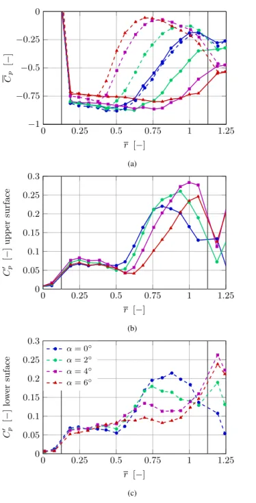
Figure5depicts the mean and standard deviation ofCpexpfor 458
angles of attack in the range 0◦ ≤ α ≤ 6◦. The distributions
459
along the upper and lower surfaces of the rectangular cylinder 460
are represented by plain and dashed lines, respectively. For the 461
sake of clarity,Cpis not depicted along the upstream face but it 462
exhibits the expected parabolic behavior aroundCp=1. 463
At zero incidence, the distribution ofCpexp is nearly identi-464
cal for the upper and lower surfaces. Starting from the leading 465
edges of the cylinder, the pressure is almost constant with only 466
a very weak decrease over the first half of the upper and lower 467
surfaces. It then increases rapidly but smoothly until the rear 468
side of the rectangular cylinder. The start of this pressure recov-469
ery is located at aroundr = 0.5. This location corresponds to 470
the core of a vortex referred to as the main vortex byBruno et al.
471
(2010) and appearing along both the upper and lower sides. In 472
particular, this main vortex is enclosed in a mean separation 473
bubble extending from the leading edge of the cylinder to the 474
point where the mean free shear layer impinges on the surface 475
and the flow reattaches. The maximum ofCp along the upper 476
and lower surfaces is located at a distance 0.94cfrom the lead-477
ing edges. As shown byRobertson et al.(1975,1978) and illus-478
trated in Sec.3.2.2, this location correlates with the point where 479
the mean flow reattachment occurs (Mannini et al.,2017), i.e. 480
the end of the main vortex 481
For non-zero incidences, increasing the angle of attack ex-482
tends the plateau region on the upper surface further down-483
stream and reduces the magnitude of the pressure recovery. Ad-484
ditionally, the pressure intensity of theCp exp
plateau region re-485
mains more or less the same for small angles of attack. As these 486
changes in the pressure distribution can be related to changes in 487
the mean flow structures, this shows that the main vortex core 488
moves downstream on the upper surface asαincreases. More-489
over, asCpexpdoes not exhibit a local maximum near the trail-490
ing edge of the cylinder, it is possible that the mean flow does 491
not reattach along the upper surface forα ≥ 2◦. Atα = 4◦, 492
the suction in the nearly constantCpregion slightly decreases, 493
which corresponds to the end of the linear region of the clexp 494
curve shown in Fig.4a. Atα = 6◦, the distribution ofCp exp 495
is nearly flat over the entire upper surface and its magnitude is 496
significantly reduced compared to lower angles of attack. This 497
is typical for a post-stall angle and explains the decrease of the 498
mean lift coefficient clexp. The opposite behavior is observed 499
on the lower surface. The extent of the plateau region and the 500
corresponding suction decrease with increasing angle of attack. 501
Moreover, the pressure recovery is more abrupt and reaches a 502
maximum value that increases and whose location moves up-503
stream withα. This behavior suggests that the mean reattach-504
ment point moves upstream with increasing angle, while the 505
mean separation bubble lying along the lower surface shortens. 506
The second order statisticC0prepresents the temporal varia-507
0 0.25 0.5 0.75 1 1.25 −1 −0.75 −0.5 −0.25 0 r [−] Cp [− ] (a) 0 0.25 0.5 0.75 1 1.25 0 0.05 0.1 0.15 0.2 0.25 0.3 r [−] C 0 p [− ] upp er surface (b) 0 0.25 0.5 0.75 1 1.25 0 0.05 0.1 0.15 0.2 0.25 0.3 r [−] C 0 p [− ] lo w er suface α= 0◦ α= 2◦ α= 4◦ α= 6◦ (c)
Figure 5: Mean (a) and standard deviation (bandc) of the pressure coefficient Cpalong the rectangle surface obtained experimentally at Re=1.1×10⁴for
different angles of attack. The vertical gray lines represent the leading and trailing edges and the coordinateris defined in Fig.2.
tion aroundCp. Therefore, a high standard deviation along a 508
particular region is representative of unsteady flow separation. 509
As depicted in Fig.5b, the distribution ofC0pexpalong the upper 510
surface can be divided into two main parts: a region with low 511
standard deviation from the leading edge tor ≈0.6, followed
512
by rapid increase and large values ofC0
pup to the trailing edge. 513
The standard deviation reaches a maximum in this second re-514
gion. Increasing the incidence extends the first region further 515
downstream and moves the location of the maximumC0
pcloser 516
to the trailing edge. The value of this maximum also increases 517
untilα=4◦, and then decreases for post-stall angles of attack. 518
The same two regions are also present on the lower surface, as 519
shown in Fig.5c. Increasing the angle of attack has however 520
the opposite effects. 521
3.2.2. Comparison between experimental andcfdresults 522
Figure6depicts theCpdistributions obtained throughurans 523
andddes. Experimental results are also shown for comparison 524
purposes. The streamlines of the mean flow obtained byurans 525
andddesare also depicted. 526
As shown in Fig.6afor 0◦ angle of attack, two symmetric 527
vortices denoted AUand ALlie along the upper and lower sur-528
faces, respectively. The flow reattachment point is located at a 529
distance 0.92cfrom the leading edge forurans and 0.94cfor 530
ddes. A distribution similar toCp exp
is obtained withurans. 531
The main difference is a shift down ofCpuranscompared to the 532
experimental distribution. Moreover, the numerically computed 533
pressure recovery begins slightly further from the leading edge 534
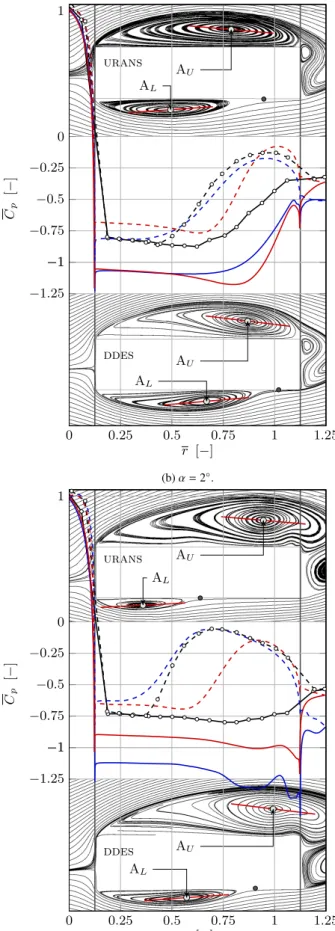
and the suction minimum occurs slightly downstream. These 535
differences can be explained by discrepancies in the estimation 536
of the mean flow features. In particular, it seems that theurans 537
vortex core of AU and AL and the reattachment points are lo-538
cated slightly downstream compared to the presumed experi-539
mental locations. As shown byWang and Gu(2015), this could 540
be explained by the sharpness of the lower edge of the exper-541
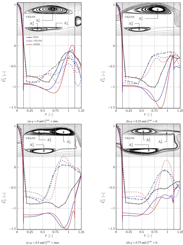
imental model compared to the numerical geometry. On the 542
other hand, the shape ofCp ddes
significantly differs fromCp exp
. 543
In particular, the plateau region is followed by a zone where the 544
suction increases before the pressure recovery and the pressure 545
recovery begins at a location much further downstream than for 546
other results. These discrepancies are caused by differences in 547
the shape of the mean vortices AU and AL. As shown by the 548
streamlines, the mean vortex cores are located further down-549
stream than forurans, which delays the pressure recovery. Ad-550
ditionally, the vortices are more tilted than for othercfdresults. 551
Therefore, the curvature of the mean streamlines is more im-552
portant below the vortex cores, which explains the suction peak 553
atr = 0.75. Finally, the mean streamlines can be compared 554
to the literature results. Theurans streamlines are similar to 555
the experimental results obtained byMizota(1981) for a sim-556
ilar case. In particular, the reattachment of the flow occurs at 557
the same location. However, this experimental study reports 558
a slightly thinner vortex with a core located atr ≈ 0.53, i.e.,
559
slightly further upstream than forurans. Conversely, the mean 560
streamlines computed withddesare very different as the prin-561
cipal axis of the main vortex is too tilted and its core is located 562
too far downstream. 563
At larger angles of attack, vortex AUgrows and moves down-564
stream, as seen in Figs.6bto6d(α = 2◦, 4◦ and 6◦). From 565
α = 2◦ the flow does not reattach along the upper surface, 566
and for α ≥ 4◦, vortex AU wraps around the trailing edge. 567
Conversely, vortex ALshrinks and is located further upstream, 568
so that the reattachment point moves forward. This behavior 569
is consistent with the conclusions drawn in Sec. 3.2.1. The 570
mean pressure distribution along the lower surface estimated 571
byuransis similar toCp exp
, despite an underestimation of the 572
suction due to vortex ALforα >2◦. On the other hand,Cp ddes
is 573
AU AL urans AU AL ddes 0 0.25 0.5 0.75 1 1.25 −1.25 −1 −0.75 −0.5 −0.25 0 1 r [−] Cp [− ] −1 exp urans ddes (a)α=0◦. AU AL urans AU AL ddes 0 0.25 0.5 0.75 1 1.25 −1.25 −1 −0.75 −0.5 −0.25 0 1 r [−] Cp [− ] −1 (b)α=2◦. AU AL urans AU AL ddes 0 0.25 0.5 0.75 1 1.25 −1.25 −1 −0.75 −0.5 −0.25 0 1 r [−] Cp [ − ] −1 (c)α=4◦. AU AL urans AU AL ddes 0 0.25 0.5 0.75 1 1.25 −1.25 −1 −0.75 −0.5 −0.25 0 1 r [−] Cp [ − ] −1 (d)α=6◦.
Figure 6: Streamlines of the mean flow calculated bycfdand mean pressure coefficientCpalong the rectangle surface obtained byurans,ddesand experimentally (exp) at Re=1.1×10⁴for different angles of attack. Plain and dashed lines correspond to the upper and lower surface, respectively. The light gray disk corresponds
very different from the experimental results, as the pressure re-574
covery begins significantly downstream. This shift is due to the 575
reattachment point and the vortex core of ALthat are estimated 576
too far downstream. The numerically computedCp along the 577
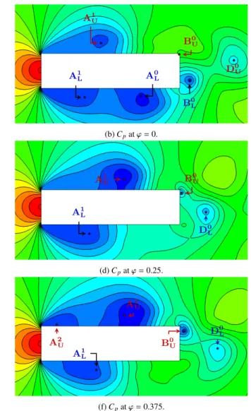
upper surface is very different fromCp exp
. The suction inten-578
sity is largely overestimated, which causes the overestimation 579
ofcldiscussed in Sec.3.1. Nonetheless, for 2◦ ≤α ≤4◦, the 580
global shape ofCp exp
along the upper surface is correctly pre-581
dicted by urans. In particular, the pressure recovery and thus 582
the location of the core of vortex AUare fairly well estimated. 583
For 2◦ ≤α ≤6◦, the pressure recovery ofCp cfd
along the up-584
per surface exhibits a non-monotonous behavior just before the 585
trailing edge. This modification in the trend ofCp is caused 586
by a small counter-rotating vortex highlighted byMannini et al.
587
(2017) which cannot be detected experimentally because of the 588
limited number of pressure taps. Atα=6◦, the flow along the
589
upper surface is better estimated byddes, as Fig.6dshows a 590
decrease of the suction intensity compared to 4◦(Fig.6c). This
591
decrease in suction is also observed forCpexp (see Sec.3.2.1) 592
and causes a decrease of the lift for incidence angles higher 593
than the stall angle. Moreover, theCpddesdistribution is nearly 594
flat, which is also the case for the experimental results. Con-595
versely, the suction intensity ofCp urans
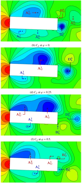
is similar for 4◦and 6◦. 596
Therefore,cluransdoes not decrease forα >4◦and
uransis not 597
able to predict the stall angle. 598
For the sake of conciseness, the standard deviations of Cp 599
obtained throughcfdare not shown. Nonetheless, the compar-600
ison between numerical and experimental results demonstrates 601
that the general shapes ofC0p depicted in Fig.5are overall re-602
trieved as long as the chordwise location of the vortex core is 603
accurately captured. However, the amplitude of C0p is largely 604
overestimated by cfd. Moreover, urans results show a non-605
physical minimum ofC0
p. These two aspects were also reported 606
byPatruno et al.(2016). 607
3.3. Spatio-temporal pressure coefficient and flow dynamics 608
This section aims to better understand the dynamics of the 609
flow by analyzing the time response of the pressure distribu-610
tion. Both experimental and numerical results are considered 611
and their respectiveCp values are compared over a shedding 612
cycle in Sec. 3.3.1. The flow dynamics is then described in 613
Sec.3.3.2. 614
3.3.1. Comparison between experimental andcfdresults 615
The experimental and numerical Cp are compared through 616
their respective approximation Cpc, which is obtained from a
617
reconstruction based on the first twodmdmodes, as explained 618
in Sec.2.3. The spatio-temporal variation ofCpcis shown for
619
α=0◦and 2◦in Figs.7and8. They depict c
Cpat four different 620
phases ϕ = t/T, where tandT are the time and the shedding
621
period, respectively. The beginning of a cycle, i.e.,ϕ=0, cor-622
responds to the minimum ofbclexp. The figures also show the 623
urans streamlines of the original flow field corresponding to 624
each phase. 625
Figure7presents the results for 0◦of incidence. As the flow 626
field is symmetrical, the accuracy of the shedding phenomenon 627
obtained numerically is assessed by comparing the variation 628
ofCpc
exp
andCpc
cfd
along the upper surface only. The dynam-629
ics along the lower surface is very similar but distant in time 630
by half a cycle. One can first observe that theurans simula-631
tion predicts better thanddesthe variation of pressure, despite a 632
consistent larger suction on the entire upper and lower surfaces. 633
Additionally, the pressure recovery starts very slightly further 634
downstream atϕ=0.25 andϕ=0.5. As already observed for 635
the mean flow, ddesresults display much larger discrepancies 636
with a larger suction peak and a pressure recovery displaced 637
downstream. This is due to a larger and more tilted vortex A1 U, 638
whose core is located further downstream. Finally, the numeri-639
cal results show larger variations in time, explaining the larger 640
standard deviation obtained withcfd. 641
For larger angles of attack (Fig.8forα=2◦), theurans pre-642
dictions are qualitatively more similar to the experimental re-643
sults than theddesestimates, but the quantitative discrepancies 644
increase with the incidence angle. This is especially the case on 645
the upper surface where suction is highly overestimated. On the 646
other hand,ddesresults show larger qualitative and quantitative 647
discrepancies. The better qualitative agreement betweenurans 648
and experiments, especially regarding the chordwise location of 649
the vortex cores and of the reattachment points, indicates that 650
uransalso provides a better representation of the flow dynam-651
ics at larger angles of attack. However, atα= 6◦ (not shown 652
here), significant discrepancies appears betweenuransand ex-653
perimental results along the upper surface anduransis not able 654
to correctly predict the flow above the rectangular cylinder. 655
3.3.2. Flow dynamics 656
The relatively good qualitative agreement betweenuransand 657
experimental results suggests thaturansis better at represent-658
ing the flow dynamics forα <6◦. Therefore, the dynamic phe-659
nomena can be qualitatively understood by analyzing the flow 660
computed byurans. In particular, Figs.9and10show the vari-661
ation of the flow around a rectangular cylinder at 0◦and 2◦of
662
incidence during a shedding cycle. 663
At 0◦ of incidence, the flow topology above and below the
664
horizontal symmetry axis of the rectangle is identical but oc-665
curs at times distant by half a shedding period. Therefore, the 666
entire dynamics is described by the time response of the flow 667
above the upper surface for 0≤ϕ≤0.5, and then by the flow
668
below the lower surface, starting back atϕ=0. Atϕ=0, and 669
as depicted by streamlines in Fig.9a, a large clockwise rotating 670
vortex, called vortex A1U, lies along the upper surface. The vor-671
ticity plot shows that the free shear layer does not impinge on 672
the rear part of the upper surface, although the flow reattaches. 673
Instead, it extends in the wake up to a zone of low pressure cor-674
responding to a previously shed vortex denoted D0
U, as depicted 675
in Fig.9b. As shown in Fig.9c, vortex A1
Uis then convected 676
downstream while the free shear layer moves closer to the sur-677
face. A clockwise rotating zone lies along the rear part of the 678
upper surface and rolls around the upper trailing edge of the 679
cylinder, forming a small vortex denoted B0
U. While vortex A 1 U 680
is being stretched and convected downstream, a new vortex A2 U 681
forms at the leading edge of the cylinder. The emergence of 682
this vortex is recognizable by the drop in pressure coefficient 683
urans A1 U 0 0.25 0.5 0.75 1 1.25 −1 −0.5 0 1 r [−] cCp [− ] expurans ddes (a)ϕ=0 andbcl exp=min. urans A1 U 0 0.25 0.5 0.75 1 1.25 −1 −0.5 0 1 r [−] cCp [− ] (b)ϕ=0.25 andbcl exp=0. urans A1 U A2 U 0 0.25 0.5 0.75 1 1.25 −1 −0.5 0 1 r [−] cCp [ − ] (c)ϕ=0.5 andbcl exp=max. urans A1 U 0 0.25 0.5 0.75 1 1.25 −1 −0.5 0 1 r [−] cCp [ − ] (d)ϕ=0.75 andbcl exp=0.
Figure 7: Distribution of the pressure coefficient reconstructed from the first twodmdmodes at four different phases of the shedding cycle for the flow around a
rectangular cylinder atα=0◦and Re=1.1×10⁴. Plain lines correspond to the upper surface. The streamlines of the original flow field obtained from uransare
also represented for easier interpretation.
near the leading edge shown in Fig.9f. Vortex A2
Uthen grows, 684
pushing vortex A1
U further downstream (lower part of Figs.9a 685 and9b), where A0 L = A 1 U and A 1 L = A 2
U. At the same time, 686
the free shear layer impinges on the upper rear corner, feed-687
ing vortex B0 U (= B
0
L), which also grows and starts to detach 688
from the rear surface. As depicted in Figs.9c and9d, where 689 D0 L =D 1 U, vortices A 1 U and B 0
U eventually merge into a single 690
vortex D1
U, which is shed into the wake. Only vortex A 2 U re-691
mains on the upper surface. Finally, vortices A2U and D1U are 692
convected downstream and a new cycle resumes. 693
Figure10ashows an overview of the flow at an incidence of 694
2◦. A large clockwise rotating vortex called vortex A1 Ucovers 695
nearly the entire upper surface atϕ=0 (Figs.10aand10b). The 696
free shear layer follows the upper part of vortex A1
Uand extends 697
into the wake until the location of a vortex called A0
U. More-698
over, a small counter-clockwise vorticity zone lies at the upper 699
trailing edge indicating the presence of a vortex called B0 U. The 700
same phase shows the emergence of a conter-clockwise rotat-701
ing vortex called A1
L at the leading edge of the lower surface. 702
Moreover, another vortex called A0
L and previously generated 703
at the leading edge is still visible on the rear part of the lower 704
surface. The free shear layer along vortices A0 L and A
1 L im-705
pinges on the rear part of the lower surface. This shear layer 706
extends further downstream, rolling around the lower trailing 707
edge and feeding the counter-clockwise rotating vortex B0L be-708
hind the rectangle. As shown in Figs.10cand10d, vortex A1U 709
elongates downstream while the upper shear layer impinges the 710
upper trailing edge and vortex B0Uis dissipated. On the lower 711
urans A1 U A1 L A2L 0 0.25 0.5 0.75 1 1.25 −1.5 −1 −0.5 0 1 r [−] cCp [− ] exp urans ddes (a)ϕ=0 andbcl exp=min. urans A1 U A2 L 0 0.25 0.5 0.75 1 1.25 −1.5 −1 −0.5 0 1 r [−] cCp [ − ] (b)ϕ=0.25 andbcl exp=0. urans A1 U A2 U A2 L 0 0.25 0.5 0.75 1 1.25 −1.5 −1 −0.5 0 1 r [−] cCp [− ] (c)ϕ=0.5 andbcl exp=max. urans A1U A2 U A2 L 0 0.25 0.5 0.75 1 1.25 −1.5 −1 −0.5 0 1 r [−] cCp [− ] (d)ϕ=0.75 andbcl exp=0.
Figure 8: Distribution of the pressure coefficient reconstructed from the first twodmdmodes at four different phases of the shedding cycle for the flow around a
rectangular cylinder atα=2◦and Re=1.1×10⁴. Plain and dashed lines correspond to the upper and lower surface, respectively. The streamlines of the original
D0 U A1 U B0U A0L A1L B0 L
(a) Streamlines andωzatϕ=0.
D0 U A1 U B0 U A0L A1 L B0L (b)Cpatϕ=0. A1 U B0 U A1 L D0L (c) Streamlines andωzatϕ=0.25. A1 U B0U A1L D0 L (d)Cpatϕ=0.25. A2U A1 U B0U A1L D0 L
(e) Streamlines andωzatϕ=0.375.
A2U A1 U B0 U A1L D0 L (f)Cpatϕ=0.375.
Figure 9: Evolution within a vortex shedding cycle of the flow around a rectangular cylinder at 0◦and Re=1.1×10⁴obtained by
urans. Left column: streamlines
and vorticity (clockwise in blue and counter-clockwise in red). Right column: pressure coefficientCp(high pressure in red and low pressure in blue) and associated
iso-contours.
surface, vortices A1Lis convected downstream while vortex A0L 712
and B0
Lmerge into a single vortex called D 0
Lwhich is shed into 713
the wake. At ϕ = 0.5 (Figs.10eand10f), a new vortex A2 U 714
forms at the upper leading edge. The upper shear layer rolls 715
around vortex A1
U and the upper trailing edge, impinging the 716
rear surface. Along the lower surface, vortex A1
L is convected 717
downstream and the free shear layer moves further away from 718
the surface. Simultaneously, a counter-clockwise vorticity zone 719
starts to form and grows into a vortex B1
Lat the lower trailing 720
edge. This vortex appears clearly in Figs. 10gand10h corre-721
sponding toϕ = 0.75. At this stage, vortex A1L lies alone on 722
the lower surface. A counter-clockwise rotating vortical zone 723
grows at the trailing edge of the upper surface and forms a 724
small vortex B1U while vortex A2U keeps growing. Simultane-725
ously, vortex A1U becomes weaker as it extends progressively 726
from the rear part of the upper surface into the wake. Vortex 727
A1
Uis finally completely shed at the end of the cycle (see vortex 728
A0
Uin Figs.10aand10b). 729
To summarize, the main dynamics consists for both cases in 730
the emergence of a vortex at the leading edge. This vortex 731
grows and is convected downstream along the surface until it 732
reaches the rear part of the cylinder and is shed into the wake. 733
However, at 0◦of incidence, the vortex generated at the leading
734
edge merges with another vortex that has grown at the trailing 735
edge. The merged vortex is then shed into the wake. For an 736
incidence of 2◦, the dynamics of the flow structures is similar
737
along the lower surface. However, it differs along the upper 738
surface where the vortex generated at the leading edge is con-739
vected and shed into the wake without merging with the vortex 740
that has appeared at the trailing edge. 741
3.4. Reynolds number effects 742
This section studies the effects of the Reynolds number on 743
the flow by analyzing the changes in the mean lift coefficient, 744
its slope and in the statistics of the pressure coefficient. 745
The mean lift coefficientclexp is represented forα =2◦ and
746
α=4◦ and several Reynolds numbers in Fig.11, that also
de-747
picts the lift slopeclexp
α calculated betweenα=0◦and 2◦. Fig-748
ure11 illustrates that an increase of the Reynolds number in 749
A0U A1U B0U A0L A1 L B0 L
(a) Streamlines andωzatϕ=0.
A0U A1U B0U A0 L A1L B0L (b)Cpatϕ=0. A1U D0 L A1 L (c) Streamlines andωzatϕ=0.25. A1 U D0 L A1 L (d)Cpatϕ=0.25. A1 U A2 U A1L B1 L D0 L
(e) Streamlines andωzatϕ=0.5.
A1 U A2 U A1L B1 L D0L (f)Cpatϕ=0.5. A1U A2U B1 U A1 L B1 L (g) Streamlines andωzatϕ=0.75. A1U A2 U B1 U A1 L B1 L (h)Cpatϕ=0.75.
Figure 10: Evolution within a vortex shedding cycle of the flow around a rectangular cylinder at 2◦and Re=1.1×10⁴obtained byurans. Left column: streamlines and vorticity (clockwise in blue and counter-clockwise in red). Right column: pressure coefficientCp(high pressure in red and low pressure in blue) and associated
iso-contours.
the range considered here leads to a significant increase of the 750
slopeclexp
α . In particular, increasing the Reynolds number from 751
7.7×10³to 1.9×10⁴leads to a relative increase of 45% of the 752
slope. This is consistent with the results reported by Schewe
753
(2013) for a 5:1 rectangular cylinder. More precisely,Schewe
754
(2013) showed a significant increase ofclαwhen increasing the 755
Reynolds number in the ranges Re<104and Re>2×10⁵, and 756
a slight decrease within 2×10⁴ <Re<105. In particular, an 757
increase of 63% of the mean lift slope atα =0◦ was reported
758
when the Reynolds number increases from 6×10³to 6×10⁴. 759
Figure12depicts the mean and the standard deviation of the 760
experimental pressure coefficient obtained at 2◦of incidence for
761
three Reynolds numbers. The main variation with the Reynolds 762
number lies in the pressure magnitude: the mean suction is 763
slightly larger on the upper surface and lower on the first and 764
last third of the lower surface (Fig.12a). Moreover, larger fluc-765
tuations, i.e., largerC0p, are observed at higher Reynolds num-766
ber (Figs.12band12c). However, the general shape of both the 767
7 692 10 513 13 590 16 282 19 231 0 0.125 0.25 0.375 0.5 clexp(α= 2◦) clexp(α= 4◦) Re [−] clexp [−] 2π 2.25π 2.5π 2.75π 3π clexpα clexpα [−]
Figure 11: Mean lift coefficient and its slope depending on Reynolds number.
mean and standard deviation does not change with the Reynolds 768
number. In particular, the location of the maximum and mini-769
mumCpexpandC0pexpremains constant. Finally, the mean pres-770
sure recovery appears to begin at the same chordwise location 771
r. 772
The changes in the magnitude of the pressure distribution, 773
and thus the higher lift, could possibly originate in the verti-774
cal displacement of the vortex cores. This could also be linked 775
to an increase/decrease of the vortex strength and/or thickness. 776
Conversely, the Reynolds number does not impact the chord-777
wise location of the two vortices as the locations of the pres-778
sure recovery along the upper and lower surfaces are constant. 779
Moreover, using the correlation of the reattachment point with 780
the maximumCp, these results indicate that the reattachment 781
point on the lower surface does not move when the Reynolds 782
number is increased, which is also supported by the location of 783
the maximum ofC0pnot being modified by Re. These results are 784
in contradiction to the mechanism proposed bySchewe(2013) 785
who suggested that the modification in the turbulence level as-786
sociated with a change of the Reynolds number induces a modi-787
fication of the flow structure along the lower surface of the rect-788
angle. More precisely,Schewe(2013) argued that an increase 789
of the Reynolds number should result in a reattachment point 790
located further upstream. The shape and curvature of the mean 791
vortex ALlocated on the lower side of the rectangular cylinder 792
would thus be modified. The subsequent change in the mean 793
pressure distribution would cause an increase of the mean lift. 794
The present results are not consistent with the mechanism pro-795
posed bySchewe(2013) but rather suggest that the lift increase 796
is related to a vertical displacement of the vortex core and/or an 797
increase in the vortex strength/thickness. 798
4. Conclusions 799
The flow around a 4:1 rectangular cylinder at several an-800
gles of attack has been studied numerically and experimentally. 801
In particular, dynamic pressure measurements have been per-802
formed to obtain the time response of the pressure coefficient 803
Cp along a cross-section of the cylinder. The pressure distri-804
bution was used to compute and study the aerodynamic loads 805 0.25 0.5 0.75 1 −1 −0.8 −0.6 −0.4 −0.2 0 r [−] Cp [− ] (a) 0.25 0.5 0.75 1 0 0.1 0.2 0.3 r [−] C 0 p [ − ] upp er surface (b) 0.25 0.5 0.75 1 0 0.05 0.1 0.15 0.2 r [−] C 0 p [ − ] lo w er surface Re = 7.7×10³ Re = 1.4×10⁴ Re = 1.9×10⁴ (c)
Figure 12: Mean and standard deviation ofCpexp atα = 2◦ depending on
Reynolds number.
on the body and to analyze the flow dynamics. The sensitiv-806
ity of the solution on the Reynolds number has been quan-807
tified by considering different Reynolds numbers ranging be-808
tween 7.8×10³and 1.9×10⁴. Additionally,
uranssimulations 809
based on thek−ωsstturbulence model andddessimulations 810
based on the Spalart-Allmaras model have been performed. The 811
pressure distribution along the cross-section of the cylinder re-812
sulting from numerical computations has been compared to the 813
experimental results through statistical analysis and a modal de-814
composition method, namelydmd. Moreover, numerical results 815
have been used to visualize key flow structures. 816
Large discrepancies between numerical and experimental re-817
sults have been highlighted. In particular, the mean suction in-818