Modeling Vortex Generators in a Navier-Stokes Code

Modeling Vortex Generators in a Navier

–

Stokes Code

Julianne C. Dudek

∗

NASA John H. Glenn Research Center at Lewis Field, Cleveland, Ohio 44135

DOI: 10.2514/1.J050683

A source-term model that simulates the effects of vortex generators was implemented into the Wind-US Navier– Stokes code. The source term added to the Navier–Stokes equations simulates the lift force that would result from a vane-type vortex generator in theflowfield. The implementation is user-friendly, requiring the user to specify only three quantities for each desired vortex generator: the range of grid points over which the force is to be applied and the planform area and angle of incidence of the physical vane. The model behavior was evaluated for subsonicflow in a rectangular duct with a single vane vortex generator, subsonicflow in an S-duct with 22 corotating vortex generators, and supersonicflow in a rectangular duct with a counter-rotating vortex-generator pair. The model was also used to successfully simulate microramps in supersonicflow by treating each microramp as a pair of vanes with opposite angles of incidence. The validation results indicate that the source-term vortex-generator model provides a useful tool for screening vortex-generator configurations and gives comparable results to solutions computed using gridded vanes.

Nomenclature

A = cross-plane area

Ap = microramp half-angle, deg

^

b = unit vector in direction of span of vortex generator c = vortex-generator chord length, mm

cVG = model constant De = exit diameter of S-duct

Di = inlet diameter of S-duct

DC60 = pressure distortion index E = total energy

FE = inviscid and viscousfluxes in energy equation

FM = inviscid and viscousfluxes in momentum equations

h = vortex-generator height, mm L = axial length of S-duct ^

l = unit vector in direction of lifting force acting onflow

Li = vortex-generator source term on celli

^

n = unit vector normal to vortex generator p = static pressure, kPa

p01 = freestream total pressure, kPa

Sj = area of cell facej

SVG = vortex-generator planform area ^

t = unit vector tangent to vortex-generator planform U = velocity,m=s

u = xvelocity

u = velocity vector ^

u = unit velocity vector Uinf = freestream velocity,m=s v = yvelocity

Vi = volume of celli

w = zvelocity

x,y,z = Cartesian coordinates

y _{= nondimensionalizedycoordinate}

= vortex-generator angle of incidence t = time step

= boundary-layer thickness, mm

,, = computational coordinates

= density

!max _{= peak vorticity}

I.

Introduction

I

N MODERN aircraft engine inlets, vortex generators (VGs) are frequently used to improve performance by minimizing the effects of adverse pressure gradients, boundary-layer separations, and shock-boundary-layer interactions. VGs come in many shapes and sizes, but in this paper, vane and microramp VGs are the focus. Vane VGs are small vane-shaped devices mounted at an angle to the localflow and introduce streamwise vortices that act to mix the high-momentumflow in the freestream with the low-momentumflow near the wall. This can be an effective means of preventing or reducing flow separation, thereby improving the performance of an inlet or wing. Microramp VGs are ramp-shaped devices that produce a pair of counter-rotating vortices that also mix the higher-momentumflow in the outer part of the boundary layer with theflow near the wall. For installation in aircraft engine inlets, microramps are sometimes more desirable than vane VGs because they are more resistant to breakage. Computationalfluid dynamics (CFD) is used to simulate inletflow and predict inlet performance and, together with experiments and statistical methods, is a useful tool in designing new inlets. Inlets occasionally include multiple VGs, and in studies where multiple VG arrays must be evaluated, it is very time consuming and impractical to generate structured computational grids for each VG. Therefore, it is highly desirable to be able to model the effects of the VGs without including their geometry in the computational mesh.

With this in mind, NASA John H. Glenn Research Center at Lewis Field (hereafter referred to as NASA Glenn) has implemented two VG models into the Wind-US Navier–Stokes code [1–3]. Previous works describe the Wendt empirical VG model and its imple-mentation [4,5]. This model was primarily developed for subsonic flows with adverse pressure gradients, and it simulates the VG by adding vorticity as a step change at a given axial station. More recently, a lift-force model, developed by Bender et al. [6], and referred to in this paper as the BAY model, was implemented into Wind-US. This is a more robust model applicable to a wider range of flows, including supersonicflows and subboundary-layer VGs. It acts over the length of the VG, rather than at a single axial station, allowing it to accurately simulate longer VGs. Both models are user-friendly; the user only needs to specify the generator location, dimensions, and angle of incidence.

In this paper, the implementation of the BAY VG model into the Wind-US code is described. The differences between the Wendt and BAY models are highlighted. Validation results for a single vane in

Presented as Paper 2010-0032 at the 48th AIAA Aerospace Sciences Meeting, Orlando, FL, 4–7 January 2010; received 24 May 2010; revision received 30 August 2010; accepted for publication 23 October 2010. This material is declared a work of the U.S. Government and is not subject to copyright protection in the United States. Copies of this paper may be made for personal or internal use, on condition that the copier pay the $10.00 per-copy fee to the Copyright Clearance Center, Inc., 222 Rosewood Drive, Danvers, MA 01923; include the code 0001-1452/11 and $10.00 in correspondence with the CCC.

∗_{Aerospace Engineer, Inlet and Nozzle Branch, 21000 Brookpark Road,} Senior Member AIAA.

AIAA JOURNAL

Vol. 49, No. 4, April 2011

equation sets governing turbulent and chemically reactingflows. The code has structured, unstructured, and hybrid grid capability, although all cases described in this paper use structured grids, and the current implementation of the VG models is valid only for structured grids. The code uses afinite volume formulation and allows the user to select from several schemes to compute both the right-hand side and left-hand side viscous terms.

Wind-US has two VG models: the Wendt model [4,5] and the recently added BAY model [6]. Both models may be used to model a single vane-type VG or an array of VGs. The Wendt model was developed primarily for subsonicflows with vanes having heights on the order of the boundary-layer thickness and having moderate height-to-chord ratios. It must be applied at a coupled zonal interface boundary, where the effects of the VGs are simulated by a step change in the secondary velocities [5]. The strength of each vortex is based on the user-input VG chord length, height, and angle of incidence with the primaryflow, as well as the local velocity and boundary-layer thickness. These VG parameters are shown in Fig. 1. The BAY model was developed to handle a wider range of VG geometric parameters, including microvanes that have small heights (25–40% of boundary-layer thickness) and vanes with large chord lengths, and it may be used in subsonic and supersonicflows. The details of the BAY model are given next.

III.

BAY Vortex Generator Model

The VG model implemented in the Wind-US Navier–Stokes code adds a source term to the momentum and energy equations that simulates the lift force introduced by a vane VG in theflowfield. This source term was developed by Bender et al. [6] and acts to align the localflow velocity with the vane VG. The BAY model has some similarities to immersed boundary methods (IBMs) [7] in that it allows the simulation of a viscousflow with immersed boundaries, the vane VGs, on grids that do not conform to the shape of the vane. It also introduces a body force that results in the desired velocityfield. It is different from an IBM in that it is not a physical boundary condition that explicitly modifies flow properties, and it is not intended to model the details of theflow on the surface of the vane, as in an IBM, but rather the effect the presence of the VG has on a given ductflow.

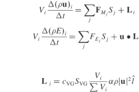
In the BAY model, the lifting force source termLiacting at grid

pointiis added to the governing discretizedfinite volume momentum and energy equations:

andl^is a unit vector in the direction of the lifting force acting on the flow. This force is equal and opposite to the force that would act on the vane. Variableuis the local velocity,is the local density,is the angle of incidence of the vane with the primaryflow,Viis the volume

of the grid cell, andViis the sum of the volumes of all of the cells

over which the model is being applied.SVGis the VG planform area, andcVGis an empirical constant. The model constantcVGcontrols the strength of the side force and the intensity with which the local velocity aligns with the vane.

The vane VG is described by three unit vectors, as shown in Fig. 2, whereb^is along the span of the vane,t^is tangent to the vane, andn^is normal to the vane and perpendicular tob^and^t. Using the small angle approximation, the unit vector l^is assumed to be normal to the velocity vector and the unit vectorb^along the VG span:

^ l u

jujb^u^b^ whereu^is a unit vector in theflow direction, and

sincos 2 u^n^ The lift-force source term is also multiplied by a factor of

^ ut^

to approximate the loss of side force at higher angles of attack. The resulting equation for the lift-force source term is

LicVGSVG Vi P Vi juj2_u^n^u^b^_u^^t (1) In [6], the value of the constantcVGwas determined by examining the integrated crossflow kinetic energyp, where

R

A_Rv2w2dA Au

2_dA

Ais the cross-plane area of the duct,vand ware the crossflow velocities, anduis the axial velocity. It was found that, for large values ofcVG,papproaches an asymptotic value because the VG model source term Li starts to dominate the other terms in the

Umax

α δ

c

h

governing equations. This causes theflow to align itself with the VG, resulting in a local angle of attack that approaches zero: i.e.,

^

un^0, so that the lift force goes to zero when the localflow becomes aligned with the vane. Reference [6] suggests that this asymptotic behavior is reached forcVG>5. Reference [8] found that theflow in an S-duct is independent of the value ofcVGfor values greater than seven. The default value forcVGin Wind-US is 10, but it may be changed by the user.

This implementation of the BAY VG model into the Wind-US code was designed to be user-friendly. The unit vectorsb^,t^, andn^are computed within the code based on the user inputs, reducing the time and effort needed to set up inputs. Within the standard Wind-US keyword inputfile, the user specifies the following information for each VG to be modeled: the range of grid points over which the model is to be applied, the planform area of the physical vane, and the angle of incidence the vane makes with the primary grid direction.

IV.

Test Cases

A. Single Vane in Subsonic Flow

Thefirst validation case run with the BAY VG model was a single vane-type VG on aflat plate in subsonic flow. For comparison,

simulations were also run with the vane gridded in the computational mesh. Results are compared with the experimental data of [9].

1. Experimental Configuration

In the experiment of interest, a single vane VG with an angle of incidence of 16 deg was mounted on a longflat plate at a location where the local boundary thicknesswas approximately 35 mm (see Fig. 3). The flow was turbulent with a freestream velocity of U35 m=s. Stereo digital particle image velocimetry measure-ments were taken using two cameras taking simultaneous pictures of the crossflow plane from opposite angles and directions. All three velocity components were obtained through stereoscopic recon-struction. The VG was a rectangularflat plate with a height of 7 mm (h=0:2) and a chord length of 49 mm (c=h7). It is considered a low-profile VG [9] (or subboundary layer VG [10]), since the height is much less than the boundary-layer thickness.

2. Computational Strategy

The boundary layer at the vane was set up by creating a long duct section (266 cm long) upstream of the specified vane location; this was the length required for the boundary-layer thickness to grow to the desired 35 mm at the vane leading edge. The model was applied at the station where35 mm. The far-field boundaries were defined to be sufficiently far from the vane to avoid influence: the grid height is 30 cm, and the grid width is 40 cm. In the experiment, the dimensions of the duct were 51 by 71 cm. A smaller computational grid was used to reduce the number of grid points, thereby reducing the computational time. Inviscid wall boundary conditions were set at the side and top boundaries. A viscous wall boundary was set at the lower wall, and the grid was clustered such thaty_{0:8at thefirst}

point from the wall. Freestream atmospheric conditions were specified at the inflow with the total temperature and pressure held

Fig. 3 Schematic of the single vane in subsonicflow test case of [9].

Fig. 4 Grid used for BAY model simulations of the Yao et al. single vane experiment [9]: a) cross-plane grid. b) isometric view showing axial grid spacing, and c) region showing grid points (in red) where the BAY model is applied.

constant. The mass flow rate at the outflow was specified as 10:75 lbm=s(4:88 kg=s). This produced the desired Mach number of 0.1 in the duct.

For the gridded vane solution, the vane had zero thickness. Two grids were created: one that was nearly identical to that used for the BAY model calculations and used inviscid boundary conditions on the vane, and another that used viscous wall boundary conditions on the vane. The latter grid was packed at the vane wall (y_{1:6) with}

viscous wall boundary conditions specified. The grid using the viscous wall boundary condition had dimensions27910164for a total of 1,803,456 grid points. The grid for the inviscid vane boundary condition case had dimensions 2799164 and 1,625,796 total points, a reduction of only 10%, since fairlyfine resolution is required to capture the vortex, as described next. In both grids, the vane grid size was22236.

Local time-stepping was used to integrate to a steady-state flowfield. The default second-order upwind-biased Roe scheme with modifications for stretched grids was used for the explicit right-hand side terms, and the default full block implicit scheme was used to compute the viscous terms. The Mentor shear stress transport (SST) turbulence model was used. The solution was considered converged when the L2 residuals had leveled off and the peak vorticity was no longer changing.

For the simulations performed using the BAY model, the model was applied to the rectangular-shaped region where the vane was located within the grid, as shown in Fig. 4c. These points envelop the region of the physical vane inclined at 16 deg and have grid dimensions22936. Generally, in the vicinity of the VG, a grid spacing of 30% of the vane chord in each coordinate direction is adequate, based on the findings in [5]. However, these recom-mendations were based on vanes that had more than double the height-to-chord ratio of the subboundary-layer vane and heights that were on the order of the boundary-layer thickness. To make sure the vortex details were captured for a vane with a smaller height, a maximum spacing of 30% of the vane height was used instead. At the vane trailing-edge tip, the resulting grid spacing in each coordinate direction wasx=h0:32,y=h0:24, andz=h0:17. To confirm that the current grid resolution was adequate, simulations were run using a grid where the number of points was halved in each direction and another grid where the number of points was doubled in each direction. The corresponding grid dimensions of the rectangular-cylinder-shaped region where the BAY model was specified were12518and441972, respectively. Based on these results, the current grid was determined to have sufficient resolution for these calculations. Doubling the number of points gave negligible benefit, while halving the grid did not provide sufficient resolution to capture the details of the vortex upstream quite as well as the chosen grid. The grid used for the model simulation is shown in Fig. 4; the cross-plane region where contours of velocity and vorticity are shown in laterfigures is also highlighted for perspective. The velocity contours’three vane heights downstream of the vane are shown for the coarse, medium, andfine grids in Fig. 5.

3. Simulation Results

Velocity contours downstream of the vane are shown for the experiment, the two gridded vane solutions, and the BAY model

solution in Fig. 6. Six axial stations are shown, measured from the vane trailing edge and nondimensionalized by the vane height. The gridded vane solution with viscous walls does the best job of simulating the vortex shape and detail forx=h10. Progressing downstream, the differences between the viscous vane solution and the inviscid vane and BAY model solutions diminish. For all stations shown, the velocity contours for the inviscid vane solution are nearly identical to those of the BAY model solution. Note that, due to limitations of the plotting software, it was not possible to match the color distribution within the velocity scale for the CFD results exactly to that shown from [9] for the experimental data; however, a best effort was made.

Vorticity contours are shown in Fig. 7 (note that three different scales are used). All simulation results underpredict the maximum vorticity magnitude, indicating a less concentrated vortex than shown experimentally. All of the simulation results are very similar in magnitude and shape, indicating that there is little benefit to using viscous wall vanes to generate a tip vortex. Note that the BAY model, unlike a viscous vane calculation, does not model the drag losses generated by the VGs and may thus give optimistic answers. For predicting these vorticity contours, the BAY model gives essentially the same result as both gridded vane solutions.

The axial decay of the peak vorticity is plotted in Fig. 8. The gridded vane solutions and the BAY model solution underpredict the initial peak vorticity shown in the experiment. The experimental value of peak vorticity at thefirst experimental measurement station atx=h1:6is approximately7200 1=s. The corresponding values for the CFD simulations are significantly less; the resulting values are 2400 1=sfor the gridded vane,2700 1=sfor the gridded vane with viscous walls, and2600 1=sfor the BAY model simulation. Of the simulations, the gridded vane solutions have slightly higher vorticity in the upstream region wherex=his between 3 and 20, but further downstream, it decays to the levels of the BAY model. This rapid decay of the peak vorticity is also seen in [9,11] and is currently unexplained.

Also, since vorticity is defined as the difference between velocity gradients, it is also very sensitive to grid resolution. To see if a grid finely packed at the location of the vane tip would significantly improve the result, a simulation was run with a grid veryfinely packed at the location of the vane tip (see Fig. 8b). The cross-plane resolution was 75%finer in the horizontal direction and 94%finer in the vertical direction. The peak vorticity resulting from the simulation using this grid is included in Fig. 8a as thefine-tip grid case. The initial peak vorticity is much higher than previous simulations; however, it also decays very quickly, as in the previous simulations. Atx=h1:6, the peak vorticity is4500 1=s. This value is closer to the experimental peak vorticity of7200 1=s, but it is still significantly lower. Another consideration is that grid refinement to this degree will not be practical in most cases, for example, in a VG screening study on a full inlet geometry with multiple VGs. And even though extensive grid resolution at the vane trailing-edge tip could potentially improve the peak vorticity near the trailing edge, it most likely will not improve the overly rapid axial decay of vorticity. Although the reasons for the discrepancy in peak vorticity between the experiment and the CFD are not fully understood, their impact on the use of the BAY model for VG screening studies is somewhat of a side issue. As the velocity contours indicate, the BAY model matched

the gridded vane results very well yet saved the user the time and labor required to grid up the vane geometry. Also, as the studies which follow will show, this discrepancy in vorticity does not negatively impact the code’s ability to predict duct performance parameters. Overall, for these calculations, the BAY model is easier to use than gridding the vanes and produces a very similar result.

B. Flow in Circular S-Duct

In this study,flow in a circular S-duct was examined for throat Mach numbers ranging from approximately 0.35 to 0.80. The purpose of the study was to evaluate Wind-US with the BAY VG model for an aggressively diffusingflow containing vane-type VGs. The results were compared with experimental data and with Wind-US simulations with the VGs represented as gridded flat plate vanes and with previous results of simulations using the Wendt VG model [5].

1. Experimental Configuration

The geometry that was tested experimentally is test case 3 from the AGARD study of [11] and was labeled the M2129 duct in the experimental investigations of [12]. The S-duct has a circular cross section and an S-shaped centerline, as shown in Fig. 9. The duct throat, which was located at the end of the upstream straight section, had a diameter Di of 5.06 in. (12.9 cm). The engine face, or

aerodynamic interface plane (AIP), was located at an axial distance ofL19:27 in:(48.9 cm); its diameterDe was 6.0 in. (15.2 cm),

and the duct vertical offsetzwas 5.4 in. (13.7 cm). The duct had a length-to-inlet diameterL=Diof 3.81, and the engine-face-to-inlet

area ratio Aef=Ai was 1.40, with an offset of z=Di1:07. A

centerbody with a cross-sectional area of about 7% of the AIP (not shown) protruded upstream from the duct outlet and extended

through the AIP. This centerbody was not modeled in the CFD investigation. A 72-probe pitot rake positioned at the engine face was used to measure the engine face total pressure recovery and distortion. It consisted of 12 six-probe rakes spaced 30 deg apart.

The VG configuration tested is referred to as VG170 in [13] and contains 11flat plate vanes per half duct, located two inlet radii downstream of the inlet throat. Each VG had a height-to-chord ratio of 0.25, where the chord was approximately 0.7 in. (18 mm), and an angle of incidence of 16 deg. The incidence was chosen in order to turn theflow near the wall away from the bottom of the duct to counteract the formation of the duct vortex.

2. Computational Strategy

The computational grids used for the simulations with the VGs gridded asflat plates and with the VG effects simulated with the VG model were very similar in terms of the number of points and clustering. The grid used for the BAY model simulations is shown in Fig. 10. Since the duct is symmetric about thex-zplane, only half of the duct was gridded. The grids include a straight 10.14-in.-long (25.76 cm) constant-area section at the upstream end of the duct, in order to allow a boundary layer to develop, and another 5.07 in. (12.88 cm) constant-area section at the downstream end, so that the computational boundary is aft of the AIP. For the gridded vane simulations, the vanes were specified using inviscid wall boundary conditions, and the grid had 718,000 points, with the sections upstream and downstream of the vane each having dimensions of 1327750 and the VG section having dimensions of 1127750. The value ofy_{at the duct wall was 0.8. The BAY}

model was specified over the 11 individual grid regions containing each VG: each region having dimensions of10225. The grid spacing at the VG trailing edge nondimensionalized by the VG chord length was 0.10 in the axial direction, 0.05 in the radial direction, and

Fig. 7 Vorticity contours at six stations downstream of VG for the experiment in [9] and three simulations.

Fig. 8 Axial decay of the peak vorticity: a) peak vorticity versus axial direction and b) cross-plane grids to illustrate grid resolution used for BAY model simulations.

0.04 in the circumferential direction. For the cases computed using the Wendt VG model, the grid was split at the vane trailing-edge station, and the Wendt model was applied at this zonal interface. For simulations using the VG models, the grid had a total of 679,000 points, 6% fewer points than used for the gridded vane. Again, afi ne-grid resolution near the vortices was desired to accurately capture the features of the vortices.

Five cases, with throat Mach numbers ranging from 0.35 to 0.80, were run with the VGs specified. The different throat Mach numbers were a result of the set value of the outflow static pressure, and the downstream pressure ratiosp=p01were those used by [14]: 0.938,

0.877, 0.861, 0.841, and 0.826. The corresponding throat Mach numbers were 0.40, 0.62, 0.68, 0.75, and 0.82.

Local time-stepping was used to integrate to a steady-state flowfield. The default second-order upwind-biased Roe scheme with modifications for stretched grids was used for the explicit right-hand side terms, and the default full block implicit scheme was used to compute the viscous terms. The Spalart–Allmaras turbulence model was used. The cases converged after approximately 15,000 iter-ations, based on the criteria that the total pressure recovery at the AIP as well as the Mach number at the throat had converged to within at least three significantfigures.

3. Results

In the discussion of results that follows, the Wind-US results computed with the BAY model are compared with experimental data

[13] and previously computed results using gridded vanes and the Wendt model [5].

The total pressure recovery versus throat Mach number is plotted in Fig. 11 for the baseline cases and for the cases with VGs in the duct. Note that neither the Wendt model nor the BAY model formulations explicitly model the total pressure losses caused by the drag forces present on the vane. This shortcoming is more apparent in the Wendt model total pressure recovery values, which are significantly higher than the experimental values, more so than the other computational results. For the lower throat Mach numbers, the VGs have little to no effect on recovery. At the higher throat Mach numbers ranging from 0.65 to 0.8, however, there is a slight increase in recovery. The VGs redistribute the low-pressureflow more uniformly around the duct, resulting in a slight improvement in the area averaged total pressure. This behavior can be better understood by examining the total pressure contours and streamline plots of Figs. 12a–12d for a throat Mach number of 0.82.

In the streamline plots shown in Figs. 12a–12d, the streamlines were released at the VG trailing-edge station, and the total pressure contours are plotted at an axial location ofx=c1, or one chord length downstream of the VG trailing edge, and at the AIP station (x=c20). The total pressure contours for the CFD solutions are shown on the computational mesh, whereas the contours for the experiment are shown using the 72-probe pitot-rake measurement locations. In the baseline case shown in Fig. 12a,flow separates on the lower surface of the duct but reattaches just upstream of the AIP; however, at the AIP, a significant low-pressure region remains at the base of the duct. This large region of low pressure results in an undesirable high level of distortion. The streamlines show that the low-pressureflow at the VG station remains near the lower surface of the duct along the axial length of the duct and through the low-pressure region at the AIP.

Fig. 9 Schematic of M2129 S-duct [13].

The total pressure contours from the experiment and the CFD solutions at the AIP show that the vanes have redistributed theflow and removed the low-pressure region at the bottom of the duct. The streamlines illustrate the movement of the low-energyflow around the circumference of the duct, resulting in an overall more uniform total pressure distribution. The BAY model AIP total pressure contour distribution gives a slightly better match to the gridded vane solution than the Wendt model result, but the two model solutions are very similar.

The DC60 distortion is plotted in Fig. 13. The DC60 distortion parameter is defined at the AIP to be the difference between the mean total pressure and the mean total pressure in the worst 60-deg sector, normalized by the mean dynamic pressure [15]. The average improvement in DC60 as a result of the addition of the VGs was 82% for the experiment, 86% for the simulations using the gridded vane, 86% for the simulations using the Wendt model, and 86% for the simulations using the BAY model. So, in terms of the DC60 distortion parameter, there appears to be no added benefit to gridding the vane versus using either VG model.

In summary, the VGs have a minimal impact on the total pressure recovery in the S-duct, with only a slight benefit at the higher throat

Mach numbers, so use of the BAY VG model versus gridded vanes makes little difference. For the distortion, the VGs greatly improve the distortion by redistributing the low-pressure region around the circumference of the duct. The results using the BAY model versus the gridded vanes were essentially equivalent; however, using the BAY model required less grid development time than gridding up vanes.

C. Counter-Rotating Vortex Generator Pair in Supersonic Flow

This validation case was run to demonstrate that the BAY model may also be used to simulate vanes in supersonic channel flow. Counter-rotating vanes in Mach 2.0flow were simulated, and results were compared with a solution computed with the vanes gridded within the computational mesh. At the time of this writing, experi-mental data for single or multiple vanes in shock-free supersonicflow could not be obtained. Data do exist for vanes in the vicinity of normal and oblique shocks; however, the computation of shock waves introduces its own challenges and may be studied in conjunction with vane VGs at a later date.

1. Configuration and Computational Strategy

Theflow conditions for this case were Mach 2.0 with a freestream velocity of 506 m=s, a total pressure of 101.4 kPa, and a total temperature of 287.2 K. The VG array consisted of two low-profile flat plate vane VGs at angles of incidence of16and 16 deg, with a chord lengthcof 36 mm and a heighthof 3.6 mm (c=h10). The leading edge of the vanes was located 100 cm from the inflow boundary where the boundary-layer thickness was 1.05 cm (h=0:34). A schematic of this configuration is shown in Fig. 14. The boundary layer at the vane was set up in a manner similar to that of the vane in subsonicflow. A long duct section (100 cm long) was created upstream of the vanes to allow the boundary-layer thickness to grow to 1.05 cm at the vane leading edge. Since the geometry was symmetric about the centerline plane between the vanes, only half of the duct was gridded, with a symmetry boundary condition applied on the plane midway between the vanes as well as on the opposite sidewall. The lower wall was specified as a viscous wall, and at thefirst grid point from the wall,y_{was equal to 0.5; the}

upper boundary was set to an inviscid wall. Inviscid wall boundary conditions were used on the vane for the gridded vane case. The inflow was set to freestream conditions, and at the outflow boundary, the pressure was extrapolated. The duct was 195 cm long, 15.25 cm high, and 2.5 cm wide. The grid had four zones. Zone 1 had dimensions of 412164, zone 2 had dimensions of 1004564, zone 3 had dimensions of214564, and zone 4 had dimensions of212164, for a total of 431,808 points. The vane was located in zone 2, and so a denser grid was used in zones 2 and 3 to capture the vortex features. The vane was specified within zone 2 and had dimensions23636.

The Wind-US code was run using local time-stepping with the Mentor SST turbulence model in a manner similar to the vane in subsonicflow. The solution was considered converged when the L2

Fig. 12 Total pressure contours forflow through an S-duct with throat Mach number of 0.82 for a) baseline case (no VGs), b) solution with gridded vanes, c) solution computed using the Wendt VG model, and d) solution computed using the BAY model.

Fig. 13 DC60 distortion at the AIP for the M2129 S-duct, shown with and without VGs.

residuals had leveled off and the area averaged total pressure recovery was changing by less than 0.0001.

2. Simulation Results

The Mach number atfive axial locations in the duct is shown in Fig. 15 for the solutions computed using the gridded vane and the BAY model. The axial stations given are nondimensionalized by the vane height. The VG pair produces a counter-rotating upward pair of

vortices, meaning that the two vortices are rotating in the upward and outward directions in the centerplane where they meet. At thefirst axial station ofx=h5, the two vortex shapes can be seen fairly distinctly. For the gridded vane case, the shape of the vortices is more clearly defined. As the vortex pair moves downstream, the two vortices move closer together and upward, away from the wall. The differences in the BAY model solution from the gridded vane solution diminish with downstream progression and, atx=h100, the shape of the Mach contours is very similar.

D. Supersonic Flow over a Microramp Vortex Generator

Microramp VGs, as shown in Fig. 16, are quite different from vane VGs in geometry. However, some of theflow physics produced by a microramp VG are similar to that produced by a pair of vanes in a counter-rotating arrangement, since both produce a counter-rotating upward pair of vortices. There are also differences in theflowfields produced by the two types of VGs; most notable is the position of the vortex shedding. The purpose of this validation case is to determine if the BAY VG model can be used to simulate microramp VGs by simulating a microramp as a pair of counter-rotating vanes.

1. Experimental Configuration

The experiment simulated was Mach 2.0 shock-freeflow over microramps, from [16]. The microramps are shown in Fig. 17 and had a heighthof 3 mm, a chord lengthcof 11 mm, and a half-angle Ap of 24 deg. Three microramps were mounted on thefloor of a

1515 cm supersonic wind tunnel at station x 13 cm and laterally spaced 25 mm apart, as measured between microramp centerlines. At this axial location, the microramp height-to-boundary-layer-thickness ratioh=was 0.26 (1:14 cm). Pitot probe measurements were taken at four downstream stations: x 8, 4, 0, and 4 cm.

2. Computational Strategy

Similar to the preceding validation case with counter-rotating vanes in supersonicflow, the boundary layer was set up by creating a long duct section (91 cm) upstream of the microramp to allow the boundary layer to grow to the desired thickness of 1.14 cm at the microramp station. Symmetry was used so only half of one microramp was modeled, and the span of the grid was 12.5 mm, which is equal to half of the distance between ramp centerlines. The height of the grid was 10 cm, which is the height of the duct used for the experiment. A symmetry boundary condition was applied on the grid plane that coincides with the microramp centerline, as well as on the opposite plane that is halfway between microramps. A viscous wall boundary condition was used on the lower wall, and thefirst grid point from the wall hady_{approximately equal to 1.0; the upper}

boundary surface was set to freestream conditions. The inflow was frozen at freestream conditions, and the outflow pressure was extrapolated. This half-microramp was simulated as a rectangular

Fig. 14 Schematic of counter-rotating VGs producing an upward vortex pair.

Fig. 15 Mach contours for a pair of counter-rotating VGs in Mach 2.0 flow for solutions computed with the gridded vane and using the BAY model.

Fig. 16 Microramp VG showing the direction of the vortices it produces.

Fig. 17 Microramp geometry parameters shown in a) top view and b) side view [16].

Fig. 18 Mach contours for a microramp in Mach 2.0flow for the experiment of [16] and the Wind-US solution computed using the BAY model. Results are shown at four axial locations.

Fig. 19 Mach number contours for a microramp in Mach 2.0flow showing results at stationx 8cmfor the experiment of [16] and for the BAY model with the vane height varied from 20–70% of the actual vane height.

vane VG using the BAY VG model. The height and chord of the vane were set to the height and chord dimensions of the microramp; however, the vane had a constant height rather than the gradually ramped-up height of the microramp. The grid had dimensions201 1944for a total of 8863 points, and the half-microramp was specified with dimensions11832.

The Wind-US code was run using local time-stepping with the Mentor SST turbulence model, as was done in the case introduced in Sec. IV.C for supersonic flow over counter-rotating vanes. The solution was considered converged when the L2 residuals had leveled off and the boundary-layer thickness at x4 cm was changing by less than 0.01%.

3. Simulation Results

The Mach number contours for both the simulation and the experiment are shown in Fig. 18 at four axial locations. The vortices produced by the BAY model are significantly larger and farther from the wall than the vortices produced by the microramps in the experiment. Vortices produced by vane VGs form at the trailing-edge tip of the vane, as shown by these simulation results. Vortices produced by microramp VGs form off the sides of the vane at some fraction of the microramp height, dependent upon the microramp geometry and the localflow conditions. Tofind out if the BAY model would better simulate the microramp vortices if the vane height were specified to be a value less than the microramp height, a series of cases were run with the vane height varied between 20 and 70% of the ramp height. The resulting Mach number contours at stationx 8 cmare shown in Fig. 19 and indicate that vane heights of 20 and 30% of the ramp height most closely match the microramp contours.

To examine this in more detail, the velocity profiles at the ramp centerline were plotted atx 8 cmin Fig. 20. By comparing the heights within the profiles where the velocity dips to a minimum value, the solution in which the vane height is 30% of the ramp height agrees best with the microramp results. Both cases show their largest velocity deficit occurring at approximately 0.45 cm from the wall, even though these minimum velocity values differ with the BAY result having a minimum velocity ratioU=Uinf of 0.66 compared with the experimental value of 0.70.

In an attempt to further improve the velocity profiles produced by the BAY model, the model constantcVGfrom Eq. (1) was varied from 1.0 to the default value of 10.0. By varying this constant, the hope was to increase the value of the minimum velocity in the deficit region to better match the experiment. The resulting Mach contours (Fig. 21) and velocity profiles (Fig. 22) were examined. As expected, for solutions where the value ofcVG>5:0, there was little change from the solution with cVG set to the default value of 10. For cVG<5:0, theylocation of the minimum velocity decreased, as did the value of the minimum velocity. So reducing the value ofcVG resulted in velocity profiles that deviated from the experiment more rather than less. Based on this, it is recommended to leavecVGset at its default value.

This validation study indicates that the BAY VG model can be used to simulate microramp VGs by specifying the microramp as two vanes at opposite angles of incidence. The vortex pair produced by the vanes occurs at the trailing-edge tip of the vanes, which tends to be further from the wall than the vortex pair produced by the microramp. To correct for this, the vane height must be specified as some fraction of the ramp height. In this case, a vane height of 30% of

Fig. 20 Velocity profiles atx 8cmfor a microramp in Mach 2.0 flow. The experiment of [16] is compared with simulation results using the BAY model with the vane heightHvspecified as 20, 30, and 100% of the microramp heightHr.

Fig. 21 Mach contours atx 8cmfor a microramp in Mach 2.0flow. Experiment of [16] is compared with simulations using the BAY model with the varying model constantcVG.

Fig. 22 Velocity profiles atx 8cmfor a microramp in Mach 2.0 flow. The experiment of [16] is compared with simulation results that used the BAY model with the model constantcVGvaried between 1.0

V.

Conclusions

A lift-force source-term VG model for vane-type VGs was implemented into the Wind-US CFD code for structured grid applications. The magnitude of the lift force is based on the localflow conditions and the size and angle of orientation of the vane. The model is user-friendly and allows the user to specify the vanes by inputting the range of grid points enveloping each vane, the planform area of the vane, and its angle of incidence. Validation results have been shown for a single vane in a subsonic channel, an S-duct with a corotating array, and a counter-rotating pair of vanes in supersonic flow. For each of these test cases, the CFD results using the model were comparable to CFD results using a gridded vane. The model was also used to successfully simulate microramps in supersonic flow by specifying the microramp as two vanes at opposite angles of incidence. Since vane VGs produce vortices at the trailing-edge tip of the VG and microramp VGs produce smaller vortices at a fraction of the microramp height, the best results in terms of the vortex size and distance from the wall were obtained when the height of the vanes was specified as 30% of the ramp height. In summary, the BAY VG model is easier to use than gridding vanes and is recommended as an efficient alternative to gridding vanes. The BAY model may also be used, with proper calibration, to simulate microramp VGs.

Acknowledgments

The author would like to sincerely thank Rodrick Chima, Mary Jo Long-Davis, and Charles Towne of the NASA John H. Glenn Research Center at Lewis Field, and Chris Nelson of Innovative Technology Applications Company, LLC.

References

[1] Bush, R. H., Power, G. D., and Towne, C. E.,“WIND: The Production Flow Solver of the NPARC Alliance,” AIAA Paper 1998-0935,

1789.

doi:10.2514/1.20141

[6] Bender, E. E., Anderson, B. H., and Yagle, P. J.,“Vortex Generator Modeling for Navier–Stokes Codes,” American Soc.of Mechanical Engineers Paper FEDSM99-6929, New York, July 1999.

[7] Fadlum, E. A., Versicco, R., and Mohd-Yusof, J.,“Combined Immersed-Boundary Finite-Difference Methods for Three-Dimensional Complex Flow Simulations,”Journal of Computational Physics, Vol. 161, No. 1, 2000, pp. 35–60.

doi:10.1006/jcph.2000.6484

[8] Jirasek, A.,“Vortex-Generator Model and Its Application to Flow Control,” Journal of Aircraft, Vol. 42, No. 6, Nov.–Dec. 2005, pp. 1486–1491.

doi:10.2514/1.12220

[9] Yao, C.-S., Lin, J. C., and Allan, B. G.,“Flow-Field Measurement of Device-Induced Embedded Streamwise Vortex on a Flat Plate,”AIAA Paper 2002-3162, June 2002.

[10] Wik, E., and Shaw, S. T.,“Numerical Simulation of Micro Vortex Generators,”AIAA Paper 2004-2697, Jan. 2004.

[11] Dudek, J. C.,“An Empirical Model for Vane-type Vortex Generators in a Navier–Stokes Code,”AIAA Paper 2005-1003, Jan. 2005.

[12] AGARD Fluid Dynamics Panel, Working Group 13,“Air Intakes for High Speed Vehicles,”AGARD AR-270, Sept. 1991.

[13] Anderson, B. H., and Gibb, J.,“Vane Effector Installation Studies on Steady State and Dynamic Inlet Distortion,”AIAA Paper 1996-3279, 1996.

[14] Mohler, R. S.,“WIND-US Flow Calculations for the M2129 S-Duct Using Structured and Unstructured Grids,”NASA CR 2003-212736, Jan. 2003.

[15] Wendt, B. J., and Dudek, J. C.,“Development of Vortex Generator Use for a Transitioning High-Speed Inlet,”Journal of Aircraft, Vol. 35, No. 4, July 1998, pp. 536–543.

doi:10.2514/2.2357

[16] Hirt, S. M., and Anderson, B. H.,“Experimental Investigation of the Application of Microramp Flow Control to an Oblique Shock Ineraction,”AIAA Paper 2009-0919, Jan. 2009.

S. Fu Associate Editor