Nonparametric Econometrics: The np Package

July 2008, Volume 27, Issue 5. http://www.jstatsoft.org/

Nonparametric Econometrics: The

np

Package

Tristen Hayfield ETH Z¨urich

Jeffrey S. Racine McMaster University

Abstract

We describe the R np package via a series of applications that may be of interest to applied econometricians. Thenppackage implements a variety of nonparametric and semiparametric kernel-based estimators that are popular among econometricians. There are also procedures for nonparametric tests of significance and consistent model speci-fication tests for parametric mean regression models and parametric quantile regression models, among others. Thenppackage focuses on kernel methods appropriate for the mix of continuous, discrete, and categorical data often found in applied settings. Data-driven methods of bandwidth selection are emphasized throughout, though we caution the user that data-driven bandwidth selection methods can be computationally demanding.

Keywords: nonparametric, semiparametric, kernel smoothing, categorical data.

1. Introduction

Devotees of R(RDevelopment Core Team 2008) are likely to be aware of a number of non-parametric kernel1 smoothing methods that exist in Rbase (e.g., density) and in certainR packages (e.g., locpolyin the KernSmooth packageWand and Ripley 2008). These routines deliver nonparametric smoothing methods to a wide audience, allowing Rusers to nonpara-metrically model a density or to conduct nonparametric local polynomial regression, by way of example.

The appeal of nonparametric methods, for applied researchers at least, lies in their ability to reveal structure in data that might be missed by classical parametric methods. Nonparametric kernel smoothing methods are often, however, much more computationally demanding than their parametric counterparts.

In applied settings we often encounter a combination of categorical and continuous datatypes. Those familiar with traditional nonparametric kernel smoothing methods will appreciate that

these methods presume that the underlying data is continuous in nature, which is frequently not the case. One approach towards handling the presence of both continuous and categorical data is called a ‘frequency’ approach, whereby data is broken up into subsets (‘cells’) corre-sponding to the values assumed by the categorical variables, and only then do you apply say densityorlocpolyto the continuous data remaining in each cell. Nonparametric frequency approaches are widely acknowledged to be unsatisfactory as they often lead to substantial efficiency losses arising from the use of sample splitting, particularly when the number of cells is large.

Recent theoretical developments offer practitioners a variety of kernel-based methods for categorical data only (i.e., unordered and ordered factors), or for a mix of continuous and categorical data. These methods have the potential to recapture the efficiency losses associated with nonparametric frequency approaches as they do not rely on sample splitting, rather, they smooth the categorical variables in an appropriate manner; see Li and Racine (2007a) and the references therein for an in-depth treatment of these methods, and see also the references listed in the bibliography.

The np package implements recently developed kernel methods that seamlessly handle the mix of continuous, unordered, and ordered factor datatypes often found in applied settings. The package also allows the user to create their own routines using high-level function calls rather than writing their ownC orFortrancode.2 _{The design philosophy underlying npaims}

to provide an intuitive, flexible, and extensible environment for applied kernel estimation. We appreciate that there exists tension among these goals, and have tried to balance these competing ends, with varying degrees of success. np is available from the ComprehensiveR Archive Network (CRAN) athttp://CRAN.R-project.org/package=np.

Currently, a range of methods can be found in the np package including unconditional (Li and Racine 2003,Ouyang, Li, and Racine 2006) and conditional (Hall, Racine, and Li 2004,

Racine, Li, and Zhu 2004) density estimation and bandwidth selection, conditional mean and gradient estimation (local constantRacine and Li 2004, Hall, Li, and Racine 2007 and local polynomialLi and Racine 2004), conditional quantile and gradient estimation (Li and Racine 2008), model specification tests (regressionHsiao, Li, and Racine 2007, quantile), significance tests (Racine 1997, Racine, Hart, and Li 2006), semiparametric regression (partially linear

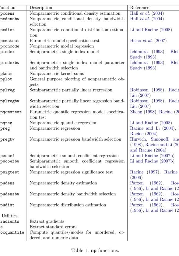
Robinson 1988, Racine and Liu 2007, index models Klein and Spady 1993, Ichimura 1993, average derivative estimation, varying/smooth coefficient modelsLi and Racine 2007b,Racine, Ouyang, and Li 2007), among others. The various functions in thenp package are described in Table1.

In this article, we illustrate the use of thenppackage via a number of empirical applications. Each application is chosen to highlight a specific econometric method in an applied setting. We begin first with a discussion of some of the features and implementation details of the

nppackage in Section2. We then proceed to illustrate the functionality of the package via a series of applications, sometimes beginning with a classical parametric method that will likely be familiar to the reader, and then performing the same analysis in a semi- or nonparametric framework. It is hoped that such comparison helps the reader quickly gauge whether or not there is any value added by moving towards a nonparametric framework for the application they have at hand. We commence with the workhorse of applied data analysis (regression)

2

The high-level functions found in the package in turn call compiledCcode allowing the user to focus on the application rather than the implementation details.

Function Description Reference npcdens Nonparametric conditional density estimation Hallet al.(2004) npcdensbw Nonparametric conditional density bandwidth

selection

Hallet al.(2004)

npcdist Nonparametric conditional distribution estima-tion

Li and Racine(2008)

npcmstest Parametric model specification test Hsiaoet al. (2007) npconmode Nonparametric modal regression

npindex Semiparametric single index model Ichimura (1993), Klein and

Spady(1993)

npindexbw Semiparametric single index model parameter and bandwidth selection

Ichimura (1993), Klein and

Spady(1993)

npksum Nonparametric kernel sums

npplot General purpose plotting of nonparametric ob-jects

npplreg Semiparametric partially linear regression Robinson (1988), Racine and

Liu(2007)

npplregbw Semiparametric partially linear regression band-width selection

Robinson (1988), Racine and

Liu(2007)

npqcmstest Parametric quantile regression model specifica-tion test

Zheng(1998),Racine(2006)

npqreg Nonparametric quantile regression Li and Racine(2008)

npreg Nonparametric regression Racine and Li (2004), Li and

Racine(2004)

npregbw Nonparametric regression bandwidth selection Hurvich, Simonoff, and Tsai

(1998),Racine and Li(2004),Li

and Racine(2004)

npscoef Semiparametric smooth coefficient regression Li and Racine(2007b) npscoefbw Semiparametric smooth coefficient regression

bandwidth selection

Li and Racine(2007b)

npsigtest Nonparametric regression significance test Racine (1997), Racine et al.

(2006)

npudens Nonparametric density estimation Parzen (1962), Rosenblatt

(1956),Li and Racine(2003)

npudensbw Nonparametric density bandwidth selection Parzen (1962), Rosenblatt

(1956),Li and Racine(2003)

npudist Nonparametric distribution estimation Parzen (1962), Rosenblatt

(1956),Li and Racine(2003)

– Utilities –

gradients Extract gradients se Extract standard errors

uocquantile Compute quantiles/modes for unordered, or-dered, and numeric data

Table 1: np functions.

in Section3, beginning with a simple univariate regression example and then moving on to a multivariate example. We then proceed to nonparametric methods for binary and multinomial outcome models in Section 4. Section 5 considers nonparametric methods for unconditional probability density function (PDF) and cumulative distribution function (CDF) estimation,

while Section6considers conditional PDF and CDF estimation, and nonparametric estimators of quantile models are considered in Section 7. A range of semiparametric models are then considered, including partially linear models in Section 8, single-index models in Section 9, and finally varying coefficient models are considered in Section10.

2. Important implementation details

In this section we describe some implementation details that may help users navigate the methods that reside in thenp package. We shall presume that the user is familiar with the traditional kernel estimation of, say, density functions (e.g., Rosenblatt 1956; Parzen 1962) and regression functions (e.g., Nadaraya 1965; Watson 1964) when the underlying data is continuous in nature. However, we do not presume familiarity with mixed-data kernel methods hence briefly describe modifications to the kernel function that are necessary to handle the mix of categorical and continuous data often encountered in applied settings. These methods, of course, collapse to the familiar estimators when all variables are continuous.

2.1. The primacy of the bandwidth

Bandwidth selection is a key aspect of sound nonparametric and semiparametric kernel esti-mation. It is the direct counterpart of model selection for parametric approaches, and should therefore not be taken lightly. np is designed from the ground up to make bandwidth selec-tion the focus of attenselec-tion. To this end, one typically begins by creating a ‘bandwidth object’ which embodies all aspects of the method, including specific kernel functions, data names, datatypes, and the like. One then passes these bandwidth objects to other functions, and those functions can grab the specifics from the bandwidth object thereby removing poten-tial inconsistencies and unnecessary repetition. For convenience these steps can be combined should the user so choose, i.e., if the first step (bandwidth selection) is not performed explic-itly then the second step will automatically call the omitted first step bandwidth selection using defaults unless otherwise specified, and the bandwidth object could then be retrieved retroactively if so desired. Note that the combined approach would not be a wise choice for certain applications such as when bootstrapping (as it would involve unnecessary computation since the bandwidths would properly be those for the original sample and not the bootstrap resamples) or when conducting quantile regression (as it would involve unnecessary computa-tion when different quantiles are computed from the same condicomputa-tional cumulative distribucomputa-tion estimate).

Work flow therefore typically proceeds as follows: 1. compute data-driven bandwidths;

2. using the bandwidth object, proceed to estimate a model and extract fitted or predicted values, standard errors, etc.;

3. optionally, plot the object.

In order to streamline the creation of a set of complicated graphics objects,plot(which calls npplot) is dynamic; i.e., you can specify, say, bootstrapped error bounds and the appropriate routines will be called in real time. Be aware, however, that bootstrap methods can be

computationally demanding hence some plots may not appear immediately in the graphics window.

2.2. Data-driven bandwidth selection methods

We caution the reader that data-driven bandwidth selection methods can be computationally demanding. We ought to also point out that data-driven (i.e., automatic) bandwidth selection procedures are not guaranteed always to produce good results due to perhaps the presence of outliers or the rounding/discretization of continuous data, among others. For this reason, we advise the reader to interrogate their bandwidth objects with the summary command which produces a table of bandwidths for the continuous variables along with a constant multiple ofσxnα, where σx is a variable’s standard deviation, n the number of observations, and α a known constant that depends on the method, kernel order, and number of continuous variables involved, e.g.,α=−1/5 for univariate density estimation with one continuous variable and a second order kernel. Seasoned practitioners can immediately assess whether undersmoothing or oversmoothing may be present by examining these constants, as the appropriate constant (called the ‘scaling factor’) that is multiplied by σxnα often ranges from between 0.5 to 1.5 for some though not all methods, and it is this constant that is computed and reported by summary. Also, the admissible range for the bandwidths for the categorical variables is provided whensummary is used, which some readers may also find helpful.

We caution users to use multistarting for any serious application (multistarting refers to restarting numerical search methods from different initial values to avoid the presence of local minima - the default is the minimum of the number of variables or 5 and can be changed via the argumentnmulti =), and do not recommend overriding default search tolerances (unless increasingnmulti =beyond its default value).

We direct the interested reader to the frequently asked questions document on the author’s website (http://socserv.mcmaster.ca/racine/np_faq.pdf) for a range of potentially help-ful tips and suggestions surrounding bandwidth selection and thenp package.

2.3. Interacting with np functions

A few words about the R data.frame construct are in order. Data frames are fundamental objects in R, defined as “tightly coupled collections of variables which share many of the properties of matrices and of lists, used as the fundamental data structure by most of R’s modeling software.” A data frame is “a matrix-like structure whose columns may be of differing types (numeric, logical, factor and character and so on).” Seasoned R users would, prior to estimation or inference, transform a given data frame into one with appropriately classed elements (the np package contains a number of datasets whose variables have already been classed appropriately). It will be seen that appropriate classing of variables is crucial in order for functions in the np package to automatically use appropriate weighting functions which differ according to a variable’s class. If your data frame contains variables that have not been classed appropriately, you can do this ‘on the fly’ by re-classing the variable upon invocation of an np function, however, it is preferable to begin with a data frame having appropriately classed elements.

There are two ways in which you can interact with functions innp, namely using data frames or using a formula interface, where appropriate. Every function innpsupports both interfaces, where appropriate.

To some, it may be natural to use the data frame interface. If you find this most natural for your project, you first create a data frame casting data according to their type (i.e., one of continuous (default),factor,ordered), as in

R> data.object <- data.frame(x1 = factor(x1), x2, x3 = ordered(x3))

wherex1 is, say, a binaryfactor,x2 continuous, andx3 an orderedfactor. Then you could pass this data frame to the appropriatenp function, say

R> bw <- npudensbw(dat = data.object)

To others, however, it may be natural to use the formula interface that is used for the regression example outlined below. For nonparametric regression functions such asnpregbw, you would proceed as you might usinglm, e.g.,

R> bw <- npregbw(y ~ x1 + x2)

except that you would of course not need to specify, e.g., polynomials in variables, interaction terms, or create a number of dummy variables for a factor. Of course, if the variables in your data frame have not been classed appropriately, then you would need to explicitly cast, say, x1via npregbw(y ~ factor(x1) + x2)above.

A few words on the formula interface are in order. We use the standard formula interface as it provides capabilities for handling missing observations and so forth. This interface, however, is simply a convenient device for telling a routine which variable is, say, the outcome and which are, say, the covariates. That is, just because one writes x1+x2 in no way means or is meant to imply that the model will be linear and additive (why use fully nonparametric methods to estimate such models in the first place?). It simply means that there are, say, two covariates in the model, the first being x1 and the second x2, we are passing them to a routine with the formula interface, and nothing more is presumed nor implied. This will likely be obvious to mostRusers, but we point it out simply to avoid any potential confusion for those unfamiliar with kernel smoothing methods.

2.4. Writing your own functions

We have tried to makenp flexible enough to be of use to a wide range of users. All options can be tweaked by the user (kernel function, kernel order, bandwidth type, estimator type and so forth). One function, npksum, allows you to create your own estimators, tests, etc. The functionnpksum is simply a call to specializedCcode, so you get the benefits of compiled code along with the power and flexibility of theRlanguage. We hope that incorporating the npksumfunction renders the package suitable for teaching and research alike.

2.5. Generalized product kernels

As noted above, traditional nonparametric kernel methods presume that the underlying data is continuous in nature, which is frequently not the case. The basic idea underlying the treatment of kernel methods in the presence of a mix of categorical and continuous data lies in the use of what we call ‘generalized product kernels’, which we briefly summarize.

Suppose that you are interested in kernel estimation for ‘unordered’ categorical data, i.e., you are presented with discrete dataXd ∈ Sd_{, whereS}d _{denotes the support ofX}d_{. We use x}d s and X_isd to denote the sth component of xd and X_id (i = 1, . . . , n), respectively. Following

Aitchison and Aitken (1976), for xd_s,X_isd ∈ {0,1, . . . , cs−1}, we define a discrete univariate kernel function

lu(X_isd, xd_s, λs) =

1−λs ifXisd =xds

λs/(cs−1) ifX_isd 6=xd_s. (1) Note that when λs = 0, l(X_isd, xd_s,0) = 1(X_isd = xd_s) becomes an indicator function, and if λs= (cs−1)/cs, thenl

X_isd, xd_s,cs−_c 1 s

= 1/cs is a constant for allvalues ofX_isd andxd_s. The range ofλs is [0,(cs−1)/cs]. Observe that these weights sum to 1.

If, instead, some of the discrete variables are ordered (i.e., are ‘ordinal categorical variables’), then we should use a kernel function which is capable of reflecting their ordered status. Assuming that xd_s can take on cs different ordered values, {0,1, . . . , cs −1}, Aitchison and Aitken(1976, p. 29) suggested using the kernel function given by

lo(xd_s, vd_s, λs) = cs j λj_s(1−λs)cs−j when |xsd−vsd|=j (0≤s≤cs), (2) where cs j = cs! j!(cs−j)!. (3)

Observe that these weights sum to 1.

If instead a variable was continuous, you could use, say, the second order Gaussian kernel, namely w(xc, X_ic, h) = √1 2π exp ( −1 2 X_ic−xc h 2) . (4)

Observe that these weights integrate to 1.

The ‘generalized product kernel function’ for a vector of, say, one unordered, one ordered, and one continuous variable is simply the product oflu(·),lo(·), andw(·), and multivariate versions with differing numbers of each datatype are created in the same fashion. We naturally allow the bandwidths to differ for each variable. For what follows, for a vector of mixed variables, we defineKγ(x, Xi) to be this product, whereγ is the vector of bandwidths (e.g., thehs and λs) and x the vector of mixed datatypes. For further details see Li and Racine (2003) who proposed the use of these generalized product kernels for unconditional density estimation and developed the underlying theory for a data-driven method of bandwidth selection for this class of estimators. The use of such kernels offers a seamless framework for kernel methods with mixed data. For further details on a range of kernel methods that employ this approach, we direct the interested reader toLi and Racine (2007a, Chapter 4).

If the user wishes to apply kernel functions other than those provided by the default set-tings, the kernel function can be changed by passing the appropriate arguments toukertype, okertype, andckertype(the first letter of each representing unordered, ordered, and contin-uous, respectively), while the ‘order’ for the continuous kernel (i.e., the first non-zero moment) can be changed by passing the appropriate (even) integer tockerorder. We support a vari-ety of unordered, ordered, and continuous kernels along with a varivari-ety of high-order kernels, the default being ckerorder = 2. Using these arguments, the user could select an eighth

order Epanechnikov kernel, a fourth order Gaussian kernel, or even a uniform kernel for the continuous variables in their application. See?npfor further details.

3. Nonparametric regression

We shall start with the workhorse of applied data analysis, namely, regression models. In order to introduce nonparametric regression, we shall first consider the simplest possible regression model, one that involves one continuous dependent variable,y, and one continuous explanatory variable,x. We shall begin with a popular parametric model of a wage equation, and then move on to a fully nonparametric regression model. Having compared and contrasted the parametric and nonparametric approach towards univariate regression, we then proceed to multivariate regression.

3.1. Univariate regression

We begin with a classic dataset taken from Pagan and Ullah (1999, p. 155) who consider Canadian cross-section wage data consisting of a random sample taken from the 1971 Cana-dian Census Public Use Tapes for male individuals having common education (Grade 13). There are n = 205 observations in total, and 2 variables, the logarithm of the individual’s wage (logwage) and their age (age). The traditional wage equation is typically modelled as a quadratic in age.

First, we begin with a simple parametric model for this relationship. R> library("np")

Nonparametric Kernel Methods for Mixed Datatypes (version 0.20-0) R> data("cps71")

R> model.par <- lm(logwage ~ age + I(age^2), data = cps71) R> summary(model.par)

Call:

lm(formula = logwage ~ age + I(age^2), data = cps71) Residuals:

Min 1Q Median 3Q Max

-2.4041 -0.1711 0.0884 0.3182 1.3940 Coefficients:

Estimate Std. Error t value Pr(>|t|) (Intercept) 10.04198 0.45600 22.02 < 2e-16 *** age 0.17313 0.02383 7.26 8.0e-12 *** I(age^2) -0.00198 0.00029 -6.82 1.0e-10 ***

Residual standard error: 0.561 on 202 degrees of freedom Multiple R-squared: 0.231, Adjusted R-squared: 0.223 F-statistic: 30.3 on 2 and 202 DF, p-value: 3.1e-12

If we first consider the model’s goodness of fit, the model has an unadjusted R2 of 23.1%. Next, we consider the local linear nonparametric method proposed by Li and Racine (2004) employing cross-validated bandwidth selection using the method of Hurvich et al. (1998). Note that in this example we conduct bandwidth selection and estimation in one step. R> model.np <- npreg(logwage ~ age, regtype = "ll", bwmethod = "cv.aic", + gradients = TRUE, data = cps71)

R> summary(model.np)

Regression Data: 205 training points, in 1 variable(s) age

Bandwidth(s): 2.81

Kernel Regression Estimator: Local-Linear Bandwidth Type: Fixed

Residual standard error: 0.272 R-squared: 0.325

Continuous Kernel Type: Second-Order Gaussian No. Continuous Explanatory Vars.: 1

Using the measure of goodness of fit introduced in the next section, we see that this method produces a better in-sample model, at least as measured by theR2 criterion, having anR2 of 32.5%.3

So far we have summarized the model’s goodness-of-fit. However, econometricians also rou-tinely report the results from tests of significance. There exist nonparametric counterparts to these tests that were proposed byRacine (1997), and extended to admit categorical variables byRacine et al. (2006), which we conduct below.

R> npsigtest(model.np)

Kernel Regression Significance Test

Type I Test with IID Bootstrap (399 replications) Explanatory variables tested for significance: age (1)

age Bandwidth(s): 2.81 Significance Tests P Value:

age <2e-16 ***

---Signif. codes: 0 '***' 0.001 '**' 0.01 '*' 0.05 '.' 0.1 ' ' 1

Having conducted this test we observe that, as was the case for the linear parametric model, the explanatory variable age is significant at all conventional levels in the local linear non-parametric model.

Assessing goodness of fit for nonparametric models

The reader may have wondered what the difference is between the R2 measures reported by the linear and nonparametric models summarized above, or perhaps how theR2was generated for the nonparametric model. It is desirable to use a unit-free measure of goodness-of-fit for nonparametric regression models which is comparable to that used for parametric regression models, namelyR2. Note that this will be awithin-samplemeasure of goodness-of-fit. Given the known drawbacks of computingR2based on the decomposition of the sum of squares (such as possible negative values), there is an alternative definition and method for computingR2 which can be used that is directly applicable to any model, linear or nonlinear. Letting yi denote the outcome and ˆyi the fitted value for observation i, we may defineR2 as follows:

R2= [ Pn

i=1(yi−y)(ˆ¯ yi−y)]¯ 2

Pn

i=1(yi−y)¯ 2Pni=1(ˆyi−y)¯2

and this measure willalways lie in the range [0,1] with the value 1 denoting a perfect fit to the sample data and 0 denoting no predictive power above that given by the unconditional mean of the outcome. It can be demonstrated that this method of computingR2 is identical to the standard measure computed asPn

i=1(ˆyi−y)¯ 2/ Pn

i=1(yi−y)¯ 2 when the model is linear,

fitted with least squares, and includes an intercept term. This useful measure will permit

direct comparison of within-sample goodness-of-fit subject to the obvious qualification that this is by no means a model selection criterion, rather, simply a summary measure that some may wish to report. This measure can, of course, also be computed using out-of-sample predictions and out-of-out-of-sample realizations. Were we to consider models estimated on a randomly selected subset of data and evaluated on an independent sample of hold-out data, this measure computed for the hold-out observations might serve to guide model selection, particularly when averaged over a number of independent hold-out datasets.

Graphical comparison of parametric and nonparametric models

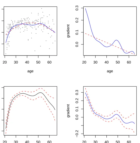
Often, a suitable graphical comparison of models allows the user to immediately appreciate features present in both the data and the estimated models.4 The upper left plot in Figure 1

presents the fitted parametric and nonparametric regression models along with the data for the cps71 example. The following code can be used to construct the plots appearing in Figure1.

R> plot(cps71$age, cps71$logwage, xlab = "age", ylab = "log(wage)", cex=.1) R> lines(cps71$age, fitted(model.np), lty = 1, col = "blue")

● ● ● ● ● ● ● ● ● ● ● ● ● ● ● ● ● ● ● ● ● ● ● ● ● ● ● ● ● ● ● ● ● ● ● ● ●● ● ● ● ● ● ● ● ● ● ● ● ● ● ● ●● ● ● ● ● ● ● ● ● ● ● ● ● ● ● ● ● ● ● ● ● ● ● ●● ● ● ● ● ● ● ● ● ● ● ● ● ● ● ● ● ●● ● ● ● ● ● ● ● ● ● ● ● ● ● ● ● ● ● ● ● ● ● ● ● ● ● ● ● ● ● ● ● ●● ● ● ● ● ● ● ● ● ● ● ● ● ● ●● ● ● ● ● ● ● ● ● ● ● ●● ● ● ● ● ● ● ● ● ● ● ● ● ● ● ● ● ● ● ● ● ● ● ● ● ● ● ● ● ● ● ● ●●● ● ● ● ● ● ● ● ● ● ● ● ● ● ● ● 20 30 40 50 60 12 13 14 15 age log(wage) 20 30 40 50 60 0.0 0.1 0.2 0.3 age gradient 20 30 40 50 60 12.0 12.5 13.0 13.5 14.0 age log(wage) 20 30 40 50 60 −0.2 0.0 0.1 0.2 0.3 age gradient

Figure 1: The figure on the upper left presents the parametric (quadratic, dashed line) and the nonparametric estimates (solid line) of the regression function for the cps71 data. The figure on the upper right presents the parametric (dashed line) and nonparametric estimates (solid line) of the gradient. The figures on the lower left and lower right present the nonpara-metric estimates of the regression function and gradient along with their variability bounds, respectively.

R> lines(cps71$age, fitted(model.par), lty = 2, col = " red") R> plot(model.np, plot.errors.method = "asymptotic")

R> plot(model.np, gradients = TRUE)

R> lines(cps71$age, coef(model.par)[2] + 2 * cps71$age * coef(model.par)[3], + lty = 2, col = "red")

The upper right plot in Figure1compares the gradients for the parametric and nonparametric models. Note that the gradient for the parametric model will be given by∂logwage_i/∂age_i= ∂βˆ2+ 2 ˆβ3agei,i= 1, . . . , n, as the model is quadratic in age.

Of course, it might be preferable to also plot error bars for the estimates, either asymptotic or resampled. We have automated this in the function npplot which is automatically called by plot. The lower left and lower right plots in Figure 1 present pointwise error bars using asymptotic standard error formulas for the regression function and gradient, respectively. Often, however, distribution free (bootstrapped) error bounds may be desired, and we allow the user to readily do so as we have writtennpto leverage thebootpackage (Canty and Ripley 2008). By default (‘iid’), bootstrap resampling is conducted pairwise on (y, X, Z) (i.e., by resampling from rows of the (y, X) data or (y, X, Z) data where appropriate). Specifying the type of bootstrapping as ‘inid’ admits general heteroskedasticity of unknown form via the wild bootstrap (Liu 1988), though it does not allow for dependence. ‘fixed’ conducts the block bootstrap (K¨unsch 1989) for dependent data, while ‘geom’ conducts the stationary bootstrap (Politis and Romano 1994).

Generating predictions from nonparametric models

Once you have obtained appropriate bandwidths and estimated a nonparametric model, gener-ating predictions is straightforward involving nothing more than cregener-ating a set of explanatory variables for which you wish to generate predictions. These can lie inside the support of the original data or outside should the user so choose. We have written our routines to support thepredictfunction inR, so by using thenewdata =option one can readily generate predic-tions. It is important to note that typically you do not have the outcome for the evaluation data, hence you need only provide the explanatory variables. However, if by chance you do have the outcome and you provide it, the routine will compute the out-of-sample summary measures of predictive ability. This would be useful when one splits a dataset into two inde-pendent samples, estimates a model on one sample, and wishes to assess its performance on the independent hold-out data.

By way of example we consider thecps71data, generate a set of values forage, two of which lie outside of the support of the data (10 and 70 years of age), and generate the parametric and nonparametric predictions using the generic predict function.

R> cps.eval <- data.frame(age = seq(10,70, by=10)) R> predict(model.par, newdata = cps.eval)

1 2 3 4 5 6 7

11.6 12.7 13.5 13.8 13.8 13.3 12.5

R> predict(model.np, newdata = cps.eval)

[1] 3.10 11.72 13.60 13.68 13.74 13.31 11.04

Note that if you provide predict with the argument se.fit = TRUE, it will also return pointwise asymptotic standard errors where appropriate.

3.2. Multivariate regression with qualitative and quantitative data

Based on the presumption that some readers will be unfamiliar with the kernel smoothing of qualitative data, we next consider a multivariate regression example that highlights the potential benefits arising from the use of kernel smoothing methods that smooth both the qualitative and quantitative variables in a particular manner. For what follows, we consider an application taken fromWooldridge(2003, p. 226) that involves multiple regression analysis with qualitative information.

We consider modeling an hourly wage equation for which the dependent variable is log(wage) (lwage) while the explanatory variables include three continuous variables, namely educ (years of education), exper (the number of years of potential experience), and tenure (the number of years with their current employer) along with two qualitative variables, female (‘Female’/‘Male’) andmarried(‘Married’/‘Notmarried’). For this example there aren= 526 observations.

The classical parametric approach towards estimating such relationships requires that one first specify the functional form of the underlying relationship. We start by first modelling this relationship using a simple parametric linear model. By way of example, Wooldridge

(2003, p. 222) presents the following model:5 R> data("wage1")

R> model.ols <- lm(lwage ~ female + married + educ + exper + tenure, + data = wage1)

R> summary(model.ols) Call:

lm(formula = lwage ~ female + married + educ + exper + tenure, data = wage1)

Residuals:

Min 1Q Median 3Q Max

-1.8725 -0.2726 -0.0378 0.2535 1.2367 Coefficients:

Estimate Std. Error t value Pr(>|t|) (Intercept) 0.33027 0.10639 3.10 0.0020 ** femaleMale 0.28553 0.03726 7.66 9.0e-14 *** marriedNotmarried -0.12574 0.03999 -3.14 0.0018 ** educ 0.08391 0.00697 12.03 < 2e-16 *** exper 0.00313 0.00168 1.86 0.0630 . tenure 0.01687 0.00296 5.71 1.9e-08 *** ---Signif. codes: 0 '***' 0.001 '**' 0.01 '*' 0.05 '.' 0.1 ' ' 1 5

We would like to thank Jeffrey Wooldridge for allowing us to incorporate his data in thenppackage. Also, we would like to point out that Wooldridge starts out with this na¨ıve linear model, but quickly moves on to a more realistic model involving nonlinearities in the continuous variables and so forth. The purpose of this example is simply to demonstrate how nonparametric models can outperform misspecified parametric models in multivariate finite-sample settings.

Residual standard error: 0.412 on 520 degrees of freedom Multiple R-squared: 0.404, Adjusted R-squared: 0.398 F-statistic: 70.4 on 5 and 520 DF, p-value: <2e-16

This model is, however, restrictive in a number of ways. First, the analyst must specify the functional form (in this case linear) for the continuous variables (educ,exper, andtenure). Second, the analyst must specify how the qualitative variables (female and married) enter the model (in this case they affect the model’s intercepts only). Third, the analyst must specify the nature of any interactions among all variables, quantitative and qualitative (in this case, there are none). Should any of these presumptions be incorrect, then the estimated model will be biased and inconsistent potentially leading to faulty inference.

One might next test the null hypothesis that this parametric linear model is correctly specified using the consistent model specification test described inHsiaoet al.(2007) that admits both categorical and continuous data (we have overridden the default search tolerances for this example as the objective function is well-behaved via tol = 0.1 and ftol = 0.1, which should not be done in general - this example will likely take a few minutes on a desktop computer as it uses bootstrapping and cross-validated bandwidth selection):

R> model.ols <- lm(lwage ~ female + married + educ + exper + tenure, + x = TRUE, y = TRUE, data = wage1)

R> output <- npcmstest(model = model.ols, tol = 0.1, ftol = 0.1,

+ xdat = model.frame(model.ols)[,-1], ydat = model.frame(model.ols)[,1]) R> summary(output)

Consistent Model Specification Test

Parametric null model: lm(formula = lwage ~ female + married + educ + exper + tenure, data = wage1, x = TRUE, y = TRUE)

Number of regressors: 5

IID Bootstrap (399 replications)

Test Statistic 'Jn': 5.6 P Value: <2e-16 ***

---Signif. codes: 0 '***' 0.001 '**' 0.01 '*' 0.05 '.' 0.1 ' ' 1 Null of correct specification is rejected at the 0.1% level

Note that it might appear at first blush that the user needs to do some redundant typing as theX data in this example is the same as the regressors in the model. However, in general Xcould differ which is why the user must specify this object separately as we cannot assume that the explanatory variables in the model will be equal toX.

This na¨ıve linear model is rejected by the data (thepvalue for the null of correct specification is<0.001), hence one might proceed instead to model this relationship using kernel methods. As noted, the traditional nonparametric approach towards modeling relationships in the pres-ence of qualitative variables requires that you first split your data into subsets containing only the continuous variables of interest (lwage,exper, andtenure). For instance, we would have four such subsets, a) n = 132 observations for married females, b) n = 120 observations

for single females, c) n= 86 observations for single males, and d) n = 188 observations for married males. One would then construct smooth nonparametric regression models for each of these subsets and proceed with analysis in this fashion. However, this may lead to a loss in efficiency due to a reduction in the sample size leading to overly variable estimates of the underlying relationship.

Instead, however, we could construct smooth nonparametric regression models by i) using a kernel function that is appropriate for the qualitative variables as outlined in Section2.5and ii) modifying the nonparametric regression model as was done byLi and Racine(2004). One can then conduct sound nonparametric estimation based on then= 526 observations rather than resorting to sample splitting. The rationale for this lies in the fact that doing so may introduce potential bias, however it will always reduce variability thus leading to potential finite-sample efficiency gains. Our experience has been that the potential benefits arising from this approach more than offset the potential costs in finite-sample settings.

Next, we consider using the local-linear nonparametric method described in Li and Racine

(2004). For the reader’s convenience we supply precomputed cross-validated bandwidths which are automatically loaded when one loads the wage1 dataset (recall being cautioned about the computational burden associated with multivariate data-driven bandwidth meth-ods).

In the example that follows, we use the precomputed bandwidth objectbw.allthat contains the data-driven bandwidths for the local linear regression produced below using all observa-tions in the sample.

R> bw.all <- npregbw(lwage ~ female + married + educ + exper + tenure, + regtype = "ll", bwmethod = "cv.aic", data = wage1)

R> model.np <- npreg(bws = bw.all) R> summary(model.np)

Regression Data: 526 training points, in 5 variable(s)

factor(female) factor(married) educ exper tenure Bandwidth(s): 0.0198 0.152 7.85 8.44 41.6 Kernel Regression Estimator: Local-Linear

Bandwidth Type: Fixed

Residual standard error: 0.137 R-squared: 0.515

Continuous Kernel Type: Second-Order Gaussian No. Continuous Explanatory Vars.: 3

Unordered Categorical Kernel Type: Aitchison and Aitken No. Unordered Categorical Explanatory Vars.: 2

Note again that the bandwidth object is the only thing you need to pass to npreg as it encapsulates the kernel types, regression method, and so forth. You could also usenpregand manually specify the bandwidths using a bandwidth vector if you so choose.6 We have tried to make each function as flexible as possible to meet the needs of a variety of users.

The goodness of fit of the nonparametric model (R2 = 51.5%) is better than that for the parametric model (R2 = 40.4%). In order to investigate whether this apparent improvement reflects overfitting or simply that the nonparametric model is in fact more faithful to the underlying data generating process, we shuffled the data and created two independent samples, one of sizen1= 400 and one of sizen2 = 126. We fit the models on then1training observations then evaluate the models on the n2 independent hold-out observations using the predicted square error criterion, namelyn−₂1Pn2

i=1(yi−yˆi)2, where theyis are the lwagevalues for the hold-out observations and the ˆyis are the predicted values. Finally, we compare the parametric model, the nonparametric model that smooths both the categorical and continuous variables, and the traditional frequency nonparametric model that breaks the data into subsets and smooths the continuous data only. For this example we use the precomputed bandwidth objectbw.subset which contains the data-driven bandwidths for a random subset of data. R> set.seed(123)

R> ii <- sample(1:nrow(wage1)) R> wage1.train <- wage1[ii[1:400],]

R> wage1.eval <- wage1[ii[401:nrow(wage1)],]

R> model.ols <- lm(lwage ~ female + married + educ + exper + tenure, + data = wage1.train)

R> fit.ols <- predict(model.ols, newdata = wage1.eval) R> pse.ols <- mean((wage1.eval$lwage - fit.ols)^2)

R> bw.subset <- npregbw(wage ~ female + married + educ + exper + tenure, + regtype = "ll", bwmethod = "cv.aic", data = wage1.train)

R> model.np <- npreg(bws = bw.subset)

R> fit.np <- predict(model.np, newdata = wage1.eval) R> pse.np <- mean((wage1.eval$lwage - fit.np)^2) R> bw.freq <- bw.subset

R> bw.freq$bw[1] <- 0 R> bw.freq$bw[2] <- 0

R> model.np.freq <- npreg(bws = bw.freq)

R> fit.np.freq <- predict(model.np.freq, newdata = wage1.eval) R> pse.np.freq <- mean((wage1.eval$lwage - fit.np.freq)^2) R> pse.ols [1] 0.147 R> pse.np [1] 0.134 R> pse.np.freq [1] 0.145

logwage) and lines(age, fitted(npreg(logwage ~ age, bws = 2))) to plot the local constant estimator with a bandwidth of 2 years).

The predicted square error on the hold-out data was 0.147 for the parametric linear model, 0.145 for the traditional nonparametric estimator that splits the data into subsets, and 0.134 for the nonparametric estimator that uses the full sample but smooths both the qualitative and quantitative data. The nonparametric model that smooths both the quantitative and qualitative data is more than 8% more efficient in terms of out-of-sample predictive ability than the parametric or frequency nonparametric model, and therefore appears to provide a better description of the underlying data generating process than either.

Note that for this example we have only four cells. If one used all qualitative and binary variables included in the dataset (sixteen in total), one would have 65,536 cells, many of which would be empty, and most having far too few observations to provide meaningful nonparametric estimates. As the number of qualitative variables increases, the difference between the estimator that smooths both continuous and discrete variables in a particular manner and the traditional estimator that relies upon sample splitting will become even more pronounced.

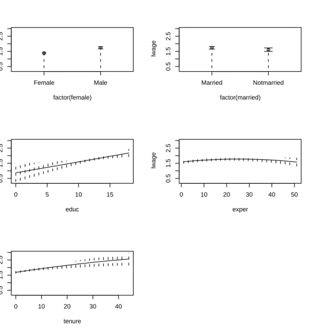
Next, we display partial regression plots in Figure 2.7 We also plot bootstrapped variability bounds, where the bootstrapping is done via theboot package thereby facilitating a variety of bootstrap methods. The following code will generate Figure2.

R> plot(model.np, plot.errors.method = "bootstrap", + plot.errors.boot.num = 25)

Figure 2 reveals that (holding other regressors constant at their median/mode), males have higher expected wages than females, there does not appear to be a significant difference between the expected wages of married and nonmarried individuals, wages increase with education and tenure and first rise then fall as experience increases, other things equal.

4. Nonparametric binary outcome and count data models

For what follows, we adopt the conditional probability estimator proposed in Hall et al. (2004) to estimate a nonparametric model of a binary outcome when there exist a number of categorical covariates.

For this example, we use the birthwt data taken from the MASS package (Venables and Ripley 2002), and compute a parametric logit model and a nonparametric conditional mode model. We then compare their confusion matrices8 and assess their classification ability. Note that many of the variables in this dataset have not been classed so we must do this upon invocation of a function. The outcome is an indicator of low infant birthweight (0/1). The method can handle unordered and ordered multinomial outcomes without modification (we have overridden the default search tolerances for this example as the objective function is well-behaved via tol = 0.1 and ftol = 0.1, which should not be done in general). In this example we first model this relationship using a simple parametric logit model, then we model this with a nonparametric conditional density estimator and compute the conditional

7

A ‘partial regression plot’ is simply a 2D plot of the outcome y versus one covariate xj when all other covariates are held constant at their respective medians/modes (this can be changed by the user).

8_{A ‘confusion matrix’ is simply a tabulation of the actual outcomes versus those predicted by a model.} The diagonal elements contain correctly predicted outcomes while the off-diagonal ones contain incorrectly predicted (confused) outcomes.

Female Male 0.5 1.5 2.5 factor(female) lwage ● ● Married Notmarried 0.5 1.5 2.5 factor(married) lwage ● _● 0 5 10 15 0.5 1.5 2.5 educ lwage 0 10 20 30 40 50 0.5 1.5 2.5 exper lwage 0 10 20 30 40 0.5 1.5 2.5 tenure lwage

Figure 2: Partial local linear nonparametric regression plots with bootstrapped pointwise error bounds for thewage1dataset.

mode, and finally, we compare confusion matrices from the logit and nonparametric models. Note that for the nonparametric estimator we conduct bandwidth selection and estimation in one step, and we first convert the data frame to one with appropriately classed elements. R> data("birthwt", package = "MASS")

R> birthwt$low <- factor(birthwt$low) R> birthwt$smoke <- factor(birthwt$smoke) R> birthwt$race <- factor(birthwt$race) R> birthwt$ht <- factor(birthwt$ht)

R> birthwt$ui <- factor(birthwt$ui) R> birthwt$ftv <- factor(birthwt$ftv)

R> model.logit <- glm(low ~ smoke + race + ht + ui + ftv + age + lwt, + family = binomial(link = logit), data = birthwt)

R> model.np <- npconmode(low ~ smoke + race + ht + ui + ftv + age + lwt, + tol = 0.1, ftol = 0.1, data = birthwt)

R> cm <- table(birthwt$low, ifelse(fitted(model.logit) > 0.5, 1, 0)) R> cm 0 1 0 119 11 1 34 25 R> summary(model.np)

Conditional Mode data: 189 training points, in 8 variable(s) (1 dependent variable(s), and 7 explanatory variable(s))

[,1] Dep. Var. Bandwidth(s): 0.0656

[,1] [,2] [,3] [,4] [,5] [,6] [,7] Exp. Var. Bandwidth(s): 0.5 0.667 0.0141 0.0325 0.542 4.98 4.45 Bandwidth Type: Fixed

Confusion Matrix Predicted Actual 0 1

0 127 3 1 25 34

Overall Correct Classification Ratio: 0.852 Correct Classification Ratio By Outcome:

0 1

0.977 0.576

McFadden-Puig-Kerschner performance measure: 0.834 Continuous Kernel Type: Second-Order Gaussian

No. Continuous Explanatory Vars.: 2

Unordered Categorical Kernel Type: Aitchison and Aitken No. Unordered Categorical Explanatory Vars.: 5

No. Unordered Categorical Dependent Vars.: 1

For this example the nonparametric model is better able to predict low birthweight infants than its parametric counterpart, correctly predicting 161/189 birthweights compared with 144/189 for the parametric model.

5. Nonparametric unconditional PDF and CDF estimation

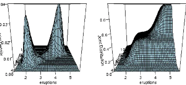
The Old Faithful Geyser is a tourist attraction located in Yellowstone National Park. This famous dataset containingn= 272 observations consists of two variables, eruption duration in minutes (eruptions) and waiting time until the next eruption in minutes (waiting). This dataset is used by the park service to model, among other things, expected duration conditional upon the amount of time that has elapsed since the previous eruption. Modeling the joint distribution is, however, of interest in its own right, and the underlying bimodal nature of the joint PDF and CDF is readily revealed by the kernel estimator. For this example, we load the old faithful geyser data and compute the density and distribution functions. To plot the conditional distribution we usecdf = TRUEinplot. Results are presented in Figure3. Note that in this example we conduct bandwidth selection and estimation in one step. R> data("faithful", package = "datasets")

R> f.faithful <- npudens(~ eruptions + waiting, data = faithful) R> summary(f.faithful)

Density Data: 272 training points, in 2 variable(s) eruptions waiting

Bandwidth(s): 0.147 2.93 Bandwidth Type: Fixed

Log Likelihood: -1106

Continuous Kernel Type: Second-Order Gaussian No. Continuous Vars.: 2

The following code will generate Figure3.

R> plot(f.faithful, xtrim = -0.2, view = "fixed", main = "")

R> plot(f.faithful, cdf = TRUE, xtrim = -0.2, view = "fixed", main = "") If one were to instead model this density with a parametric model such as the bivariate normal (being symmetric, unimodal, and monotonically decreasing away from the mode), one would of course fail to uncover the underlying structure readily revealed by the kernel estimate.

6. Nonparametric conditional PDF and CDF estimation

We consider Giovanni Baiocchi’s (Baiocchi 2006) Italian GDP growth panel for 21 regions covering the period 1951–1998 (millions of Lire, 1990 = base). There are n= 1,008 obser-vations in total, and two variables, gdpand year. First, we compute the bandwidths. Note that this may take a minute or two depending on the speed of your computer. We override the default tolerances for the search method as the objective function is well-behaved (do not of course do this in general), then we compute the npcdens object. To plot the conditional distribution we usecdf = TRUE in plot. Note that in this example we conduct bandwidth selection and estimation in one step.

Figure 3: Nonparametric multivariate PDF and CDF estimates for the Old Faithful data.

R> data("Italy")

R> fhat <- npcdens(gdp ~ year, tol = 0.1, ftol = 0.1, data = Italy) R> summary(fhat)

Conditional Density Data: 1008 training points, in 2 variable(s) (1 dependent variable(s), and 1 explanatory variable(s))

gdp Dep. Var. Bandwidth(s): 0.753 year Exp. Var. Bandwidth(s): 0.669 Bandwidth Type: Fixed

Log Likelihood: -2560

Continuous Kernel Type: Second-Order Gaussian No. Continuous Dependent Vars.: 1

Ordered Categorical Kernel Type: Wang and Van Ryzin No. Ordered Categorical Explanatory Vars.: 1

Figure 4 plots the resulting conditional PDF and CDF for the Italy GDP panel. The following code will generate Figure4.

R> plot(fhat, view = "fixed", main = "", theta = 300, phi = 50)

R> plot(fhat, cdf = TRUE, view = "fixed", main = "", theta = 300, phi = 50) Figure4reveals that the distribution of income has evolved from a unimodal one in the early 1950s to a markedly bimodal one in the 1990s. This result is robust to bandwidth choice, and

Figure 4: Nonparametric conditional PDF and CDF estimates for the Italian GDP panel.

is observed whether using simple rules-of-thumb or data-driven methods such as likelihood cross-validation. The kernel method readily reveals this evolution which might easily be missed were one to use parametric models of the income distribution (e.g., the unimodal lognormal distribution is commonly used to model income distributions).

7. Nonparametric quantile regression

We again consider Giovanni Baiocchi’s Italian GDP growth panel. First, we compute the likelihood cross-validation bandwidths (default). We override the default tolerances for the search method as the objective function is well-behaved (do not of course do this in general). Then we compute the resulting conditional quantile estimates using the method of Li and Racine(2008). By way of example, we compute the 25th, 50th, and 75th conditional quantiles. Note that this may take a minute or two depending on the speed of your computer. Note that for this example we first call npcdensbw to avoid unnecessary re-computation of the bandwidth object.

R> bw <- npcdensbw(gdp ~ year, tol = 0.1, ftol = 0.1, data = Italy) R> model.q0.25 <- npqreg(bws = bw, tau = 0.25)

R> model.q0.50 <- npqreg(bws = bw, tau = 0.50) R> model.q0.75 <- npqreg(bws = bw, tau = 0.75)

Figure 5 plots the resulting quantile estimates. The following code will generate Figure5. R> plot(Italy$year, Italy$gdp, main = "", xlab = "Year",

+ ylab = "GDP Quantiles")

R> lines(Italy$year, model.q0.25$quantile, col = "red", lty = 1, lwd = 2) R> lines(Italy$year, model.q0.50$quantile, col = "blue", lty = 2, lwd = 2)

● 1951 1957 1963 1969 1975 1981 1987 1993 5 10 15 20 25 30 Year GDP Quantiles tau = 0.25 tau = 0.50 tau = 0.75

Figure 5: Nonparametric quantile regression on the Italian GDP panel.

R> lines(Italy$year, model.q0.75$quantile, col = "red", lty = 3, lwd = 2) R> legend(ordered(1951), 32, c("tau = 0.25", "tau = 0.50", "tau = 0.75"), + lty = c(1, 2, 3), col = c("red", "blue", "red"))

One nice feature of this application is that the explanatory variable is ordered and there exist multiple observations per year. Using theplotfunction with ordered data produces a boxplot which readily reveals the non-smooth 25th, 50th, and 75th quantiles. These non-smooth quantile estimates can then be directly compared to those obtained via direct estimation of the smooth CDF which are plotted in Figure5.

8. Semiparametric partially linear models

Suppose that we consider thewage1dataset fromWooldridge(2003, p. 222), but now assume that the researcher is unwilling to presume the nature of the relationship betweenexperand lwage, hence relegates experto the nonparametric part of a semiparametric partially linear model. The partially linear model was proposed byRobinson(1988) and extended to handle the presence of categorical covariates byRacine and Liu (2007).

Before proceeding, we ought to clarify a common misunderstanding about partially linear models. Many believe that, as the model is apparently simple, its computation ought to also be simple. However, the apparent simplicity hides the perhaps under-appreciated fact that bandwidth selection for partially linear models can be orders of magnitude more com-putationally burdensome than that for fully nonparametric models, for one simple reason.

Data-driven bandwidth selection methods such as cross-validation are being used, and the partially linear model involves cross-validation to regressyonZ (Z is multivariate) theneach

column of X on Z, whereas fully nonparametric regression involves cross-validation of y on

X only. The computational burden associated with partially linear models is therefore much more demanding than for nonparametric models, so be forewarned. Note that in this example we conduct bandwidth selection and estimation in one step.

R> model.pl <- npplreg(lwage ~ female + married + educ + tenure | exper, + data = wage1)

R> summary(model.pl) Partially Linear Model

Regression data: 526 training points, in 5 variable(s)

With 4 linear parametric regressor(s), 1 nonparametric regressor(s) y(z) Bandwidth(s): 2.05 x(z) Bandwidth(s): 4.194 1.353 3.161 0.765

female married educ tenure Coefficient(s): 0.29 -0.0372 0.0788 0.0166 Kernel Regression Estimator: Local-Constant Bandwidth Type: Fixed

Residual standard error: 0.155 R-squared: 0.449

A comparison of this model with the parametric and nonparametric models presented in Section3.2indicates an in-sample fit (44.9%) that lies in between the misspecified parametric model (40.4%) and the fully nonparametric model (51.5%).

9. Semiparametric single-index models

9.1. Binary outcomes (Klein-Spady with cross-validation)

We could again consider the birthwt data taken from the MASS package, and this time compute a semiparametric index model. We then compare confusion matrices and assess classification ability. The outcome is an indicator of low infant birthweight (0/1). We apply the method of Klein and Spady (1993) with bandwidths selected via cross-validation. Note that for this example we conduct bandwidth selection and estimation in one step

R> model.index <- npindex(low ~ smoke + race + ht + ui + ftv + age + lwt, + method = "kleinspady", gradients = TRUE, data = birthwt)

R> summary(model.index) Single Index Model

Regression Data: 189 training points, in 7 variable(s)

smoke race ht ui ftv age lwt

Beta: 1 0.0816 0.378 0.188 0.00651 -0.00385 -0.00233 Bandwidth: 0.0525

Kernel Regression Estimator: Local-Constant Confusion Matrix

Predicted Actual 0 1

0 127 3 1 47 12

Overall Correct Classification Ratio: 0.735 Correct Classification Ratio By Outcome:

0 1

0.977 0.203

McFadden-Puig-Kerschner performance measure: 0.673 Continuous Kernel Type: Second-Order Gaussian

No. Continuous Explanatory Vars.: 1

It is interesting to compare this with the parametric logit model’s confusion matrix presented in Section 4. A comparison of this model with the parametric model presented in Section 4

reveals that it correctly classifies an additional 5/189 observations. 9.2. Continuous outcomes (Ichimura with cross-validation)

Next, we consider applying Ichimura (1993)’s single-index method which is appropriate for continuous outcomes, unlike that ofKlein and Spady(1993) (we override the default number of multistarts for the user’s convenience as the global minimum appears to have been located in the first attempt). We again consider thewage1dataset found inWooldridge(2003, p. 222). Note that in this example we conduct bandwidth selection and estimation in one step. R> model <- npindex(lwage ~ female + married + educ + exper + tenure, + data = wage1, nmulti = 1)

R> summary(model) Single Index Model

female married educ exper tenure Beta: 1 -0.106 0.0599 0.00121 0.0143 Bandwidth: 0.0732

Kernel Regression Estimator: Local-Constant Residual standard error: 0.161

R-squared: 0.431

Continuous Kernel Type: Second-Order Gaussian No. Continuous Explanatory Vars.: 1

It is interesting to compare this model with the parametric and nonparametric models pre-sented in Section3.2as it provides an in-sample fit (43.1%) that lies in between the misspec-ified parametric model (40.4%) and fully nonparametric model (51.5%). Whether this model yields improved out-of-sample predictions could also be explored.

10. Semiparametric varying coefficient models

We revisit the wage1 dataset found in Wooldridge (2003, p. 222), but assume that the re-searcher believes that the model’s parameters may differ depending on one’s sex. In this case, one might adopt a varying coefficient approach such as that found in Li and Racine

(2007b) andRacineet al.(2007). We compare a simple linear model with the semiparametric varying coefficient model. Note that the X data in the varying coefficient model must be of type numeric, so we create a 0/1 dummy variable from the qualitative variable for X, but of course for the nonparametric component we can simply treat these as unordered factors. Note that we do bandwidth selection and estimation in one step.

R> model.ols <- lm(lwage ~ female + married + educ + exper + tenure, + data = wage1)

R> wage1.augmented <- wage1

R> wage1.augmented$dfemale <- as.integer(wage1$female == "Male")

R> wage1.augmented$dmarried <- as.integer(wage1$married == "Notmarried") R> model.scoef <- npscoef(lwage ~ dfemale + dmarried + educ + exper + + tenure | female, betas = TRUE, data = wage1.augmented)

R> summary(model.scoef) Smooth Coefficient Model

Regression data: 526 training points, in 1 variable(s) female

Bandwidth(s): 0.104 Bandwidth Type: Fixed

Residual standard error: 0.162 R-squared: 0.426

Unordered Categorical Kernel Type: Aitchison and Aitken No. Unordered Categorical Explanatory Vars.: 1

R> colMeans(coef(model.scoef))

Intercept dfemale dmarried educ exper tenure 0.33419 0.28878 -0.13370 0.08407 0.00338 0.01515 R> coef(model.ols)

(Intercept) femaleMale marriedNotmarried educ

0.33027 0.28553 -0.12574 0.08391

exper tenure

0.00313 0.01687

It is again interesting to compare this model with the parametric and nonparametric models presented in Section 3.2. It can be seen that the average values of the model’s coefficients are in agreement with those from the linear specification, while the in-sample goodness of fit (42.6%) lies in between the misspecified parametric model (40.4%) and fully nonparametric model (51.5%).

11. Writing your own kernel-based functions

The functionnpksum exists so that you can create your own kernel objects with or without a variable to be weighted (defaults to 1). With the options available, you could create new nonparametric tests or even new kernel estimators. The convolution kernel option would allow you to create, say, the least squares cross-validation function for kernel density estimation. npksum implements a variety of methods for computing multivariate kernel sums (p-variate) defined over a set of possibly continuous and/or discrete data.

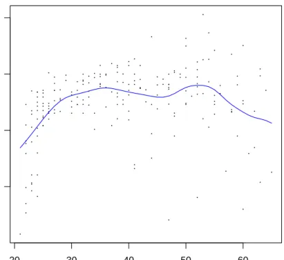
By way of example, we construct a local constant kernel estimator with a bandwidth of, say, two years. Figure6 plots the resulting estimate.

R> fit.lc <- npksum(txdat = cps71$age, tydat = cps71$logwage, bws = 2)$ksum/ + npksum(txdat = cps71$age, bws = 2)$ksum

The following code will generate Figure6.

R> plot(cps71$age, cps71$logwage, xlab = "Age", ylab = "log(wage)") R> lines(cps71$age, fit.lc, col = "blue")

npksum is exceedingly flexible, allowing for leave-one-out sums, weighted sums of matrices, raising the kernel function to different powers, the use of convolution kernels, and so forth. See?npksumfor further details.

● ● ● ● ● ● ● ● ● ● ● ● ● ● ● ● ● ● ● ● ● ● ● ● ● ● ● ● ● ● ● ● ● ● ● ● ●● ● ● ● ● ● ● ● ● ● ● ● ● ● ● ●● ● ● ● ● ● ● ● ● ● ● ● ● ● ● ● ● ● ● ● ● ● ● ● ● ● ● ● ● ● ● ● ● ● ● ● ● ● ● ● ● ●● ● ● ● ● ● ● ● ● ● ● ● ● ● ● ● ● ● ● ● ● ● ● ● ● ● ● ● ● ● ● ● ●● ● ● ● ● ● ● ● ● ● ● ● ● ● ● ● ● ● ● ● ● ● ● ● ● ● ● ● ● ● ● ● ● ● ● ● ● ● ● ● ● ● ● ● ● ● ● ● ● ● ● ● ● ● ● ● ● ● ● ● ●● ● ● ● ● ● ● ● ● ● ● ● ● ● ● ● 20 30 40 50 60 12 13 14 15 Age log(wage)

Figure 6: A local constant kernel estimator generated withnpksum for thecps71 dataset.

12. A parallel implementation

Data-driven bandwidth selection methods are, by their nature, computationally burdensome. However, many bandwidth selection methods lend themselves well to parallel computing ap-proaches. High performance computing resources are becoming widely available, and multiple CPU desktop systems have become the norm and will continue to make inroads.

When users have a large amount of data, serial bandwidth selection procedures can be infea-sible. For this reason, we have developed anMPI-aware version of the np package that uses some of the functionality of theRmpipackage which we have tentatively called the npRmpi

package and is available from the authors upon request (the Message Passing Interface (MPI) is an open library specification for parallel computation available for a range of computing platforms). The functionality of np and npRmpi is identical, however, using npRmpi you could take advantage of a cluster computing environment or a multi-core/multi-CPU desk-top machine thereby alleviating the computational burden associated with the nonparametric analysis of large datasets. Installation of this package, however, requires knowledge that goes beyond that which even seasonedRusers may possess. Having access to local expertise would be necessary for many users therefore this package is not available via CRAN.

13. Summary

Thenppackage offers users of Ra variety of nonparametric and semiparametric kernel-based methods that are capable of handling the mix of categorical and continuous data typically encountered by applied researchers. In this article we have described the functionality of the np package via a series of illustrative applications that may be of interest to applied econometricians interested in becoming familiar with these methods. We do not delve into details of the underlying estimators, rather we provide references where appropriate and direct the interested reader to those resources.

The help files accompanying many functions found in the np package contain numerous ex-amples which may be of interest to some readers, and we encourage readers to experiment with these examples in addition to those contained herein.

Finally, we encourage readers who have successfully implemented new kernel-based methods using thenpksum function to send such functions to us so that they can be included in future versions of thenp package with appropriate acknowledgment of course.

Acknowledgments

We are indebted to Achim Zeileis and to two anonymous referees whose comments and feed-back have resulted in numerous improvements to thenppackage and to the exposition of this article. Racine would like to gratefully acknowledge support from the Natural Sciences and Engineering Research Council of Canada (http://www.nserc.ca/), the Social Sciences and Humanities Research Council of Canada (http://www.sshrc.ca/), and the Shared Hierar-chical Academic Research Computing Network (http://www.sharcnet.ca/).

References

Aitchison J, Aitken CGG (1976). “Multivariate Binary Discrimination by the Kernel Method.”

Biometrika,63(3), 413–420.

Baiocchi G (2006). Economic Applications of Nonparametric Methods. Ph.D. thesis, Univer-sity of York.

Canty A, Ripley BD (2008). boot: Functions and Datasets for Bootstrapping. R package version 1.2-33, URLhttp://CRAN.R-project.org/package=boot.

Hall P, Li Q, Racine JS (2007). “Nonparametric Estimation of Regression Functions in the Presence of Irrelevant Regressors.”The Review of Economics and Statistics,89, 784–789. Hall P, Racine JS, Li Q (2004). “Cross-Validation and the Estimation of Conditional

Proba-bility Densities.”Journal of the American Statistical Association,99(468), 1015–1026. Hsiao C, Li Q, Racine JS (2007). “A Consistent Model Specification Test with Mixed

Cate-gorical and Continuous Data.”Journal of Econometrics,140, 802–826.

Hurvich CM, Simonoff JS, Tsai CL (1998). “Smoothing Parameter Selection in Nonparametric Regression Using an Improved Akaike information criterion.”Journal of the Royal Statistical

Ichimura H (1993). “Semiparametric Least Squares (SLS) and Weighted SLS Estimation of Single-Index Models.”Journal of Econometrics,58, 71–120.

Klein RW, Spady RH (1993). “An Efficient Semiparametric Estimator for Binary Response Models.”Econometrica,61, 387–421.

K¨unsch HR (1989). “The Jackknife and the Bootstrap for General Stationary Observations.”

The Annals of Statistics,17(3), 1217–1241.

Li Q, Racine JS (2003). “Nonparametric Estimation of Distributions with Categorical and Continuous Data.”Journal of Multivariate Analysis,86, 266–292.

Li Q, Racine JS (2004). “Cross-Validated Local Linear Nonparametric Regression.”Statistica

Sinica,14(2), 485–512.

Li Q, Racine JS (2007a). Nonparametric Econometrics: Theory and Practice. Princeton University Press.

Li Q, Racine JS (2007b). “Smooth Varying-Coefficient Nonparametric Models for Qualitative and Quantitative Data.” Unpublished Manuscript, McMaster University and Texas A&M University.

Li Q, Racine JS (2008). “Nonparametric Estimation of Conditional CDF and Quantile Func-tions with Mixed Categorical and Continuous Data.” Journal of Business & Economic

Statistics. Forthcoming.

Liu RY (1988). “Bootstrap Procedures Under Some Non I.I.D. Models.” The Annals of

Statistics,16, 1696–1708.

Nadaraya EA (1965). “On Nonparametric Estimates of Density Functions and regression curves.”Theory of Applied Probability,10, 186–190.

Ouyang D, Li Q, Racine JS (2006). “Cross-Validation and the Estimation of Probability Distributions with Categorical Data.”Journal of Nonparametric Statistics,18(1), 69–100. Pagan A, Ullah A (1999). Nonparametric Econometrics. Cambridge University Press, New

York.

Parzen E (1962). “On Estimation of a Probability Density Function and Mode.”The Annals

of Mathematical Statistics,33, 1065–1076.

Politis DN, Romano JP (1994). “Limit Theorems for Weakly Dependent Hilbert Space Valued Random Variables with Applications to the Stationary Bootstrap.” Statistica Sinica, 4, 461–476.

Racine JS (1997). “Consistent Significance Testing for Nonparametric Regression.” Journal

of Business & Economic Statistics,15(3), 369–379.

Racine JS (2006). “Consistent Specification Testing of Heteroskedastic Parametric Regression Quantile Models with Mixed Data.” Unpublished Manuscript, McMaster University. Racine JS, Hart JD, Li Q (2006). “Testing the Significance of Categorical Predictor Variables

Racine JS, Li Q (2004). “Nonparametric Estimation of Regression Functions with Both Categorical and Continuous Data.” Journal of Econometrics,119(1), 99–130.

Racine JS, Li Q, Zhu X (2004). “Kernel Estimation of Multivariate Conditional Distributions.”

Annals of Economics and Finance,5(2), 211–235.

Racine JS, Liu L (2007). “A Partially Linear Kernel Estimator for Categorical Data.” Un-published manuscript, McMaster University.

Racine JS, Ouyang D, Li Q (2007). “Nonparametric Multilevel Models: A Smoothing Ap-proach.” Unpublished Manuscript, McMaster University and Texas A&M University. RDevelopment Core Team (2008).R: A Language and Environment for Statistical Computing.

RFoundation for Statistical Computing, Vienna, Austria. ISBN 3-900051-07-0, URLhttp: //www.R-project.org/.

Robinson PM (1988). “Root-N Consistent Semiparametric Regression.” Econometrica, 56, 931–954.

Rosenblatt M (1956). “Remarks on some Nonparametric Estimates of a Density Function.”

The Annals of Mathematical Statistics,27, 832–837.

Venables WN, Ripley BD (2002). Modern Applied Statistics with S. 4th edition. Springer-Verlag, New York.

Wand M, Ripley B (2008). KernSmooth: Functions for Kernel Smoothing. R package version 2.22-22, URLhttp://CRAN.R-project.org/package=KernSmooth.

Watson GS (1964). “Smooth Regression Analysis.” Sankhya,26:15, 359–372. Wooldridge JM (2003). Introductory Econometrics. Thompson South-Western.

Zheng J (1998). “A Consistent Nonparametric Test of Parametric Regression Models Under Conditional Quantile Restrictions.”Econometric Theory,14, 123–138.

Affiliation: Tristen Hayfield ETH Z¨urich H¨onggerberg Campus Physics Department CH-8093 Z¨urich, Switzerland E-mail: [email protected] URL: http://www.exp-astro.phys.ethz.ch/hayfield/

Jeffrey S. Racine

Department of Economics McMaster University

Hamilton, Ontario, Canada, L8S 4L8 E-mail: [email protected]

URL:http://http://www.mcmaster.ca/economics/racine/

Journal of Statistical Software

http://www.jstatsoft.org/ published by the American Statistical Association http://www.amstat.org/

Volume 27, Issue 5 Submitted: 2007-04-30