www.ssoar.info
Sampling in Theory (Version 2.0)
Gabler, Siegfried; Häder, Sabine
Erstveröffentlichung / Primary Publication Arbeitspapier / working paper
Zur Verfügung gestellt in Kooperation mit / provided in cooperation with:
GESIS - Leibniz-Institut für Sozialwissenschaften
Empfohlene Zitierung / Suggested Citation:
Gabler, S., & Häder, S. (2016). Sampling in Theory (Version 2.0). (GESIS Survey Guidelines). Mannheim: GESIS -Leibniz-Institut für Sozialwissenschaften. https://doi.org/10.15465/gesis-sg_en_008
Nutzungsbedingungen:
Dieser Text wird unter einer CC BY-NC-ND Lizenz (Namensnennung-Nicht-kommerziell-Keine Bearbeitung) zur Verfügung gestellt. Nähere Auskünfte zu den CC-Lizenzen finden Sie hier:
https://creativecommons.org/licenses/by-nc-nd/4.0/deed.de
Terms of use:
This document is made available under a CC BY-NC-ND Licence (Attribution-Non Comercial-NoDerivatives). For more Information see:
Leibniz-Institut
für Sozialwissenschaften
GESIS Survey Guidelines
Sampling in Theory
Siegfried Gabler & Sabine Hader
Abstract
This contribution addresses the theoretical foundations o f sampling. It begins with an introduction to sampling terminology, and discusses terms such as target population, frame population, and sampling
frame. It then deals individually with the different types o f random sampling, presenting the formulae for simple random sampling, stratified and systematic random sampling, cluster sampling, two-stage sampling procedures, and sampling procedures with unequal inclusion probabilities. And finally, it explains how the necessary sample size is determined.
Citation
Gabler, S., ft Häder, S. (2016). Sampling in Theory. GESIS Survey Guidelines. Mannheim, Germany: GESIS - Leibniz Institute for the Social Sciences, doi: 10.15465/gesis-sg_en_009
1. What ¡s ¡t all about?
Because the inclusion o f all units o f a population o f interest is usually far too expensive and time intensive, survey researchers lim it themselves to a certain number o f representatives (i.e., a sample) in order to be able to make statements about characteristics o f that population. The Norwegian statistician Anders Nicolai Kiaer was the first to propose such a "representative method," which he presented at a conference o f the International Statistical Institute in 1895. Initially, however, Kiser's proposal did not meet with widespread peer approval, but rather it triggered a dispute. Nonetheless, with time, sample surveys increasingly prevailed in national statistical agency practice. At the same time, work continued on the theoretical foundations - the theory - o f sampling. It was V.P. Godambe (1955) who finally gave sampling unified theoretical foundations. By now, it would be hard to imagine life without sample surveys. We encounter them practically everywhere. Especially in the run-up to elections, for example, there is frequent speculation about how polling organisations actually arrive at their election forecasts. The theoretical foundations required to answer this and other questions will be addressed in what follows.
2. Which is better: A sample or a census?
Suppose we are interested in one characteristic o f a population, for example the mean net income of the households in the German city o f Mannheim. How can we obtain this information?
• We can ask all households in Mannheim about their net income and then compute the mean. • We can select a number of Mannheim households and ask them to give us information about
their net income. If the households are selected according to certain rules, we can then make a statistical inference from the sample to the population and, with a certain degree of probability, draw conclusions about the mean net income o f all households in Mannheim. Hence, when the objective is to procure information about a population, we have two options: a census or a sample.
The advantage o f a census - that is, a survey o f every element in a population - is that the parameters o f interest can be stated precisely. In the above-mentioned example, our result would be: The mean net household income in Mannheim is EURX.
If the parameter was estimated on the basis o f a sample, the result would be expressed in a more complicated way. For example: With a probability o f 95°/o, the mean net household income in Mannheim is EUR X ± EUR Y. Clearly, the result obtained on the basis o f a sample survey is considerably more complex and not "completely certain".
So why is a census not conducted in every ease? The reason is that sample surveys have a number of definite advantages:
• They are less costly than censuses.
• The results o f a sample survey are available more quickly than those o f a census.
• Less staff are needed to conduct a sample survey than a census. More specific training can be provided to the staff o f a sample survey.
• Nonresponse, for example because respondents cannot be reached, can be dealt with better in sample surveys than In censuses. Hence, in the case o f a sample survey, the number o f contact attempts can be Increased to four or five. In the case o f a census, this would be very cost intensive. Associated with this Is the - at first glance paradoxical - fact that sample surveys may have a higher level of measurement accuracy than surveys planned as censuses.
• Sometimes, sample surveys are the only way o f obtaining Information about the population of Interest. This Is the case, for example, when the object o f Investigation Is destroyed during measurement (e.g., when measuring the lifetime o f a light bulb as an element o f quality control).
• The overall burden on respondents is smaller because fewer people are asked to provide Information.
However, there are also circumstances in which the use o f sample surveys Is not an appropriate option. In the case o f relatively small populations (e.g., Л/ = 30), for example, It generally makes little sense to draw a sample. A census Is also more appropriate when one wishes to make statements about small sub-populations within a population. This is because such statements may be very imprecise if they are made on the basis o f a sample survey as the number of sampling units Is too small. A census Is also to be recommended when it Is known in advance that the population Is very heterogeneous. Fingerprints (the pattern o f the papillary ridges on the finger tips) are one example of a population that Is extremely heterogeneous with regard to one characteristic. It can be assumed that no two fingerprints In the world are Identical.
In certain eases - for example, motor vehicle recall campaigns - a survey sample is Impossible and a census Is the only option.
3. What terms are important?
The total set of units for which the Information derived from the sample is supposed to be valid is known as the target population. At the beginning o f the Investigation, the substantive, geographical, and temporal bounds o f this population must be clearly defined.
Example: A telephone survey Is to be conducted to determine how changes In telecommunication behaviour affect social relationships. To this end, the target population Is first delimited to Include all persons who can be reached by telephone. The second substantive delimitation Is German-speaking, which Is also based on practical considerations relating to the planned telephone survey.
Substantive delimitation: All German-speaking persons who can be reached by landline or mobile phone,
Geographical delimitation: who live in the Federal Republic o f Germany, and Temporal delimitation: who are aged 16 years or older (In the case o f younger
persons, the consent o f a parent or guardian would be required).
The next step entails researching whether a sampling frame exists In which the elements of the target population are recorded In an acceptable way.
In this context, acceptable means that the sampling frame is sufficiently up-to-date. Example: The municipal population registers normally have a time lag - that Is, they contain errors with regard to
mobile persons, births, and deaths. This was made clear, for example, by the 2011 Census, which showed that Germany had around 1.5 million less inhabitants than was assumed on the basis o f the population register figures and the intercensal population updates (register error). Nonetheless, population registers are frequently used because a better sampling frame is not available. Up-to-date means:
• Each element in the target population Is present once and only once - that is, the frame does not exhibit overcoverage (i.e., the presence of elements that do not belong to the target population) or undercoverage (i.e., the absence of elements that belong to the target population).
• The sampling frame is accessible for the survey and is not too costly to use. (In the case of the population registers, for example, the Investigation must be In the public Interest. In other words, samples of persons are not made available for just any research topic. Moreover, the research institute must be able to produce a current clearance certification (see Albers, 1997, p. 118T). The prices for samples from population registers are laid down by the respective federal states (Länder] and vary quite considerably.
Ideally, the frame population and the target population are identical. In practice, however, this is very rarely the ease. It is therefore necessary to evaluate the differences between the target population and the frame population. In general, the problem is less pronounced when the deviations are random rather than systematic - that is, when they do not relate to variables o f interest to the investigation. For example, the telephone book is not suitable for use as a sampling frame for nationwide surveys in Germany because of the high percentage o f unlisted telephone subscribers. By contrast, the telephone book might be quite a suitable sampling frame for surveys in a rural region of Southwestern Germany, where almost all households are still listed.
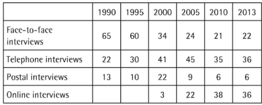
And finally, in order to be able to assess whether it makes sense to conduct a sample survey, the size of the target population must be estimated before the investigation begins. This is particularly important when a suitable sampling frame is not available and the sample must therefore be recruited by means o f screening. Take, for example, a project conducted in the year 2000, to which GESIS acted as an adviser. Within the framework o f that project a nationwide survey was to be carried out o f parents with children aged eight years or less. Population registers could not be used as a sampling frame because the sample had to be as unclustered as possible. This is best achieved by means of telephone screening. On the basis o f figures from the 1998 Microeensus, it was calculated that the percentage of households with children under the age o f nine should be 13°/o in Western Germany and 11% in Eastern Germany. However, a pretest revealed that only 7.4°/o o f the households contacted by telephone in Western Germany and only 4.6°/o o f households contacted by telephone in Eastern Germany had a child under the age o f nine. The targeted net sample size was n = 1,500 in Western and Eastern Germany respectively. Therefore, it would have been necessary to contact 20,271 households in Western Germany and 32,609 households in Eastern Germany. However, these figures are based on the assumption that all o f these households would have been willing to participate in the survey. Proceeding on the more realistic assumption that only around half the selected households could actually have been contacted and would have been willing to participate in the survey, over 100,000 telephone calls would have been needed in order to recruit the targeted number o f cases. Whether a survey institute is in a position to carry out such a task, or whether a different approach must be taken to handling the research topic, depends on the institute's financial, staffing, and technical resources. In market and social research, a trend has set in in recent years whereby less face-to-face interviews and more online interviews are being conducted. This is clearly illustrated by the following figures for the number of interviews conducted by the member institutes o f the Arbeitskreis Deutscher Markt- und Sozialforsehungsinstitute (ADM; http://www.adm-ev.de/), the association that represents the interests
o f the main commercial market and social research agencies in Germany. The advantages and disadvantages o f the different survey modes cannot be discussed here. However, the reader is referred to the contributions in the "Survey Design" section o f the GESIS Survey Guidelines.
Table 1. Quantitative interviews conducted by the member institutes o f the ADM by interview type (in o/o) 1990 1995 2000 2005 2010 2013 Faee-to-faee interviews 65 60 34 24 21 22 Telephone interviews 22 30 41 45 35 36 Postal interviews 13 10 22 9 6 6 Online interviews 3 22 38 36
4. What are random samples and what types of random samples are there?
Generally speaking, there are different ways of drawing a sample from a population. They include: • Simple random sampling
• Stratified random sampling • Systematic random sampling • Cluster sampling
• Two-stage sampling procedures
• Sampling procedures with unequal inclusion probabilities
If, for example, an acceptable sampling frame exists, a simple random sample or, if additional information is available, a stratified random sample can be drawn. The survey mode is irrelevant here. In other words, these sampling mechanisms can be applied in the case o f all survey modes (postal, faee- to-face, telephone, or online).
If, on the other hand, a suitable sampling frame is not available, a substitute construction must be used, for example a multi-stage area sample with random-route elements.
In what follows, the theoretical foundations o f the various types o f random samples will be presented. Proof o f the statements can be found, for example, in Lohr (1999) and Särndal (1992).
Simple random sampling
When selecting units from a population, it is beneficial to draw them according to a law o f probability because statistically sound statements can then be made about population parameters o f interest to the researcher.
Let us first assume that only one unit is to be selected from a population comprising Л/ units and that each unit has an equal probability of selection - namely, 1/N. The selection o f the unit can realised by means of a random experiment.
If we repeat this random experiment independently n times, and note the selected units in a vector (/q, . , where I k denotes the unit selected in the kth repetition o f the random experiment (i.e., the kth draw), there are 1 /N ” different equally probable outcomes. This sampling design is also known as simple random sampling with replacement (SRSWR) .
_ 1 n
The sample mean у = — £ Y¡ is a random variable with Пк=-\ к
EsJ f i = Y ^ - - ^ Y k
N jt=i —\2 ( H = v with varc, 1 JV. n N k=yAn unbiased estimator usrswr for the variance o f the sample mean is given by
2
5 7 1 n i _\2
o srswr = — with s = ---^ (У / “ И as the (corrected) sample variance.
n n - h = i k ’
Therefore, for large samples o f size n,
is the 95°/o confidence interval for the unknown population mean o f interest Y .
If a unit selected in the /th draw no longer has a positive probability o f being selected again in subsequent draws, and if all those units that have not been selected by the /th draw have the same probability of being selected in the remaining draws, this is referred to as simple random sampling w ithout replacement (SRSWOR, or the short form SRS in what follows).
_ 1 n
The sample mean у = — £ Y¡ is a random variable with Пк=] k
52 ( n \ ■> 1 n Z _Ч2
и = — 1--- with s = --- £1Г, - / ) as the (corrected) sample variance.
nA N п - П = Л “ '
s i , n \ ... 9 1 JL n < N J n - \ k = - \ Therefore, for large samples comprising n units
is the 95°/o confidence interval for the unknown population mean o f interest, Y . n
If the sampling fraction n/N is small - say, less than 5°/o - the correction factor ^1 - — J is often neglected and the formulae for sampling with replacement are used.
An important special case exists when each у can take on only the values 0 or 1, and Y can be interpreted as a proportion value. In this case, P is often written instead o f Y . Analogously, the sample mean is denoted by p. The variance cr2 can be written as ст2 = P(1-P) and s2 = —— p (1 -p ). Because o f the great importance o f proportion values, the formulae are explicitly cited here:
n -1
In the case o f simple random sampling with replacement,
e
,„M=
p
var,
n
An unbiased estimator usrswr for the variance o f the sample proportion p is given by u.
For large samples comprising n elements, p -1.9 6 ,Г 4' ;p +1.96,
n - 1
is the 95°/o confidence interval for the unknown population mean o f interest, P. Because n is large, n-1 can also be replaced with n.
In the case o f simple random sampling w ithout replacement,
E , M = P
var
Á
p
) =
P ( l - P ) < n - 1 n < N - 1 JAn unbiased estimator u srs for the variance o f the sample proportion p is given by
srs n -1 N
is the 95°/o confidence interval for the unknown population mean o f interest, P. When N and n are large, Л/-1 can be replaced with Л/and n-1 can be replaced with n.
Stratified random sampling
Target populations are often naturally stratified, and samples are drawn independently in different strata. If a simple random sample is drawn, and if N ( h ) and n (h ) denote the size of the target population and of the sample from the hth stratum (h='\,...,H) respectively, the weighted arithmetic mean of the sample mean y(/?) is used as an estimator. More specifically, for
y(h)
Estr ( y st r ) = Y
An unbiased estimator Vstr for the variance o f the stratified estimator is given by = " ( W(/l)V S2(/7)< n(/l)
Vstr~ i k N
J
n(h)L
N (h ))'Therefore, for large samples comprising n(h) elements, [ V s t r — 1 ■ 9 6 -'J v str 'Y s t r + 1-96 J
is the 95°/o confidence interval for the unknown population mean o f interest, Y .
Three possible ways o f allocating a sample comprising n elements to strata are typically cited: Proportional allocation n[h] = ---n N Optimal allocation n(h) = n ■ N (h )J ? (h ) X W(gX/s2(g) 9=1 Cost-optimal allocation n(/,) = c . N(h)yjs2(h)c(h) X N(gY]s2(g)c(g) 9=1 _ H _
where с(Л) are the mean costs o f surveying a unit in the hth stratum and с = X n(h)c(h) is the total
/j=i
If the mean costs are the same for each stratum, cost-optimal allocation becomes optimal allocation. If the variances o f the / values in the strata are equally large, optimal allocation becomes proportional allocation. In the ease o f proportional allocation, the stratified estimator and the sample mean are identical.
Why stratify?
As can be seen from the formula for the variance o f the stratified estimator
the variance is small when the variation o f the / values within the strata is low. In such cases a stratification gain is realised by using the stratified sample mean rather than the simple random sample mean.
Systematic random sampling
In systematic random sampling, the population of N = nH units is, as a rule, first arranged in some order according to one or several variables. A starting number, K, is then randomly chosen, where 1 < К < H. The units with the numbers К, K+H,..., K+(n-'\)H are then selected. Thus, for the estimator the following holds true
_ 1 n
У sys =
_ 2
YK +¡H П ,'=1^ s y s ( ^ s y s ) —
va rs/s
(ysys) =
(1 + (n - Dp ).
where p is the intra-class correlation coefficient that can be interpreted as a correlation coefficient between pairs o f units within the same (systematic) sample, that is,
P =
í
S
(Yk+iH ~Y)(Yk+jH-И
k=ti,j=Oi*J__________________
(n-D(/v-DS2
An unbiased estimator for the variance does not exist. Because — n -1
< p < 1 , vars/s( / s/s) can be , N - 1
between 0 and S ---. The extreme value 0 occurs when all the sample means o f the systematic N
samples are the same. The other extreme case occurs when all the / values in a systematic sample are the same. In the ease o f simple random sampling, varsys(ysys) clearly corresponds to the variance of
1 the sample mean when p =
Systematic random sampling is a special case o f cluster sampling.
Cluster sampling
Let us assume that the population is - as in the ease o f stratification - divided into H clusters, where N h is the size o f the hth cluster. A simple random sample o f n clusters is drawn. As an estimator for
= 1 H _ H
Y = — ¿ NhYh with К = ¿ Nh we use
К h=1 /7=1
H H _
Vc l= —
2
LhNhYh nK h = twhere Yh is the mean of the у values in the hth cluster (h = and
Lh
1 if the /?th cluster is selected 0 otherwise
Then
Ed (Vcl) = Y
varc, f c ) = | ( l - ^ with % .
If n>1,an unbiased estimator o cl for varc, (y c/) is given by
with
H
n \ H n - 1 h = i
Two-stage sampling procedure
Stratified sampling and cluster sampling are two special cases o f the two-stage sampling procedure. The population comprises N primary sampling units (PSUs). Let the /th primary sampling unit contain M¡ secondary sampling units (SSUs). Let F, denote the i value o f the variable o f interest in the /th PSU. Further, we define - M, = 1 N N - ■> 1 W / —\2 9 r- = 4 4 - = L V = - r . S ¡
= —
S
Г - И y=1к
7=1 l \ IV - 1 /=1 ' ' /И;Z - 42 W with K = X M i1
7=1 7=1 1Assuming that a simple random sample o f n PSUs is drawn without replacement and a simple random sample o f m¡ SSUs is also drawn without replacement from the /th PSU,
and
l-i
Then
1 if the /fh secondary unit in the /* 0 otherwise
fh
1 if th e / primary unit is selected 0 otherwise EY = Y va r Y =
J_
F
j _F
primary unit is selected
(/ = 1..../V). n N J n m A Mi N 2 i | s t2 + y ¿ M 2— 1 1 -Л/ t „ Z—< ' ' ™ m : JJ N
m
N n ¡ ( / = = 1,...,Л/) _ 1 MiYi = — X ¿,7^7 is the sample mean in the /th PSU, m,. ;=i J J
Sampling procedure with unequal inclusion probabilities
Let denote the probability that the /th and the yth element o f the target population will be selected. Instead o f 7TU, we write яу. The Horvitz-Thompson estimator is used as an unbiased estimator for the
N
sum Y =
У'
XN у Y ' нт
= Y
/ , 4l
A
l
with L: = <1 if the unit is selected 0 otherwise
for
i =
.
It is assumed that all яу are positive. The variance o f the Horvitz-Thompson estimator is
N N у Y.
v a r ( F ) = £ £ “ ( ^ - ^ ) X 7 /=1 7=1
In the case o f a sampling procedure with a fixed sample size n,
N N N
2 л-,у = пл, und Z Z л„- = n
7=1 ,=17=1
and the so-called Yates-Grundy variance estimator
yields an unbiased estimate o f the var(V H7-) when all are positive. It is clearly non-negative when > Tty applies to all /' Ф j.
In the case o f simple random sampling, л-,у = 77777— 7 for /#/ and ^, =77- The Horvitz-Thompson N
/V(/V-1)
1 'h
estimator is then N times the sample mean. In the case o f stratified random sampling, л, = — for /' in Nh
_"I j
the hth stratum. For /'#/' both in the hth stratum, л,7 = \ h— Ț and otherwise л,. = 7Г,7Г,.
IJ Nh[Nh - i ) 1] 1 1
Determining the necessary sample size in the case of simple random sampling (SRS)
We find ourselves in the following situation: The tolerable sampling error and the significance level are specified - for example, with a level o f significance o f 5°/o, the population proportion should not deviate by more than ± 3 percentage points from the point estimator.So, how large must the sample be?
Let
nsrs be the sample size under SRS N be the size o f the target population
Za/2 be the tabulated value from the standard normal distribution; for a = 0.05, ^ / 2 = 1-96
p be the proportion o f the variable o f interest in the sample, known either from a previous investigation or worst case p = 0.5
e be the permissible absolute sampling error; 2e corresponds to the length o f the confidence interval
Estimation o f proportion values in the case o f a small sampling fraction (n/N < 0,05)
nsrs • p • (1 - p)
Estimation o f proportion values in the case o f a large sampling fraction
Taking into account the correction factor 1 - — (selection without replacement)
nsrs
N - z 2
a,2 • p
(1-pQ
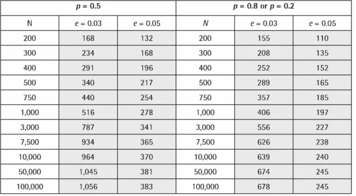
Table 2. Minimum sample size n for specified absolute sampling error e with significance level a = 0.05 for proportions p = 0.5 and p = 0.8
(or p = 0.2) (following Borg 2000, p. 144)
p = 0.5 p = 0.8 or p = 0.2 N e = 0.03 e = 0.05 N e = 0.03 e = 0.05 200 168 132 200 155 110 300 234 168 300 208 135 400 291 196 400 252 152 500 340 217 500 289 165 750 440 254 750 357 185 1,000 516 278 1,000 406 197 3,000 787 341 3,000 556 227 7,500 934 365 7,500 626 238 10,000 964 370 10,000 639 240 50,000 1,045 381 50,000 674 245 100,000 1,056 383 100,000 678 245
Determination of the necessary sample size in the case of complex sampling designs
In the case o f complex sampling designs, there is usually an increase in variance as a result o f clustering and weighting. This should be taken into account when determining the necessary sample size. The design effect is a measure of this change of variance.n kOmpi = n srs ■
Deff
To compute design effects (Kish 1965, 1980, 1987)
Deff = VI v0
where
V is the variance o f the estimator under a complex samplingldesign v0 is the variance o f the estimator under SRS
(There are advantages in using the variance o f the estimator under SRSWR.)
When determining the (model-based) design effect for complex sampling designs, two components must be taken into account: the design effect due to clustering and the design effect due to unequal inclusion probabilities (Kish 1987; Proof: Gabler/Häder/Lahiri 1999)
X niwi _ _
D e ff = n -Ț -i--- [1 + (ö - 1)p] = (1 + £) [1 + [b - 1)p] = D e ff, ■ Deffc /=1
where
n, is the number o f observations in the /th weighting class w¡ are the weights in the /th weighting class
n = 2Ln( is the sample size i=i
b is the mean cluster size
p is the intra-class correlation coefficient
With regard to the magnitude o f design effects that occur in survey practice, Kish (1987) notes: "Variations o f 1.0 to 3.0 of deft are common ..." whereby Deft = yjDeff . In the ESS, a design effect Deffw o f around 1.2 was observed in different countries in different years in the case o f samples with equal inclusion probabilities at the household level in which unequal inclusion probabilities occurred only at the last sampling stage - the selection o f the target person in the household (Ganninger 2010).
References
Borg, I. (2000). Führungsinstrum ent M itarbeiterbefragung: Theorien, Tools und Praxiserfahrungen. Göttingen: Verlag fü r Angewandte Psychologie.
Gabler, S., Hader, S., Et Lahiri, P. (1999). A model based ju stifica tio n o f Kish's formula for design effects for weighting and clustering. Survey M ethodology Vol. 25, No.1.
Ganninger, M. (2010). Design effects: Model-based versus design-based approach. GTSIS SehriftenreiheMol. 3.
Godambe, V. P. (1955). A unified theory o f sampling from fin ite populations. Journal o f the Royal S tatistica l Society 17, Series B: 269-278.
Kish, L. (1965). Survey sampling. New York: Wiley.
Kish, L. (1987). Weighting in Deft2. The Survey S tatistician. June 1987. Lohr, S. L, (1999). Sampling: Design and analysis. Duxbury Press
Särndal, C-E, Swensson, B., Et Wretman, J, (1992). Model assisted survey sampling. New York: Springer Verlag.