The Weak Instrument Problem of the
System GMM Estimator in Dynamic
Panel Data Models
Maurice J.G. Bun
Frank Windmeijer
Discussion Paper No. 07/595
March 2007
Department of Economics
University of Bristol
The Weak Instrument Problem of the System GMM
Estimator in Dynamic Panel Data Models
∗
Maurice J.G. Bun
Dept. of Quantitative Economics
University of Amsterdam
[email protected]
Frank Windmeijer
Dept. of Economics
University of Bristol
and cemmap/IFS
[email protected]
March, 2007
AbstractThe system GMM estimator for dynamic panel data models combines moment conditions for the model infirst differences with moment conditions for the model in levels. It has been shown to improve on the GMM estimator in thefirst differenced model in terms of bias and root mean squared error. However, we show in this paper that in the covariance stationary panel data AR(1) model the expected values of the concentration parameters in the differenced and levels equations for the cross-section at time t are the same when the variances of the individual heterogeneity and idiosyncratic errors are the same. This indicates a weak instrument problem also for the equation in levels. We show that the 2SLS biases relative to that of the OLS biases are then similar for the equations in differences and levels, as are the size distortions of the Wald tests. These results are shown in a Monte Carlo study to extend to the panel data system GMM estimator.
JEL Classification: C12, C13, C23
Keywords: Dynamic Panel Data, System GMM, Weak Instruments
∗Helpful comments were provided by Steve Bond and Jon Temple. This paper has been presented at the13th Panel Data Conference in Cambridge, Amsterdam, Copenhagen, cemmap and Bristol.
1
Introduction
A commonly employed estimation procedure to estimate the parameters in a dynamic panel data model with unobserved individual specific heterogeneity is to transform the model into first differences. Sequential moment conditions are then used where lagged levels of the variables are instruments for the endogenous differences and the parameters estimated by GMM, see Arellano and Bond (1991). It has been well documented (see e.g. Blundell and Bond (1998)) that this GMM estimator in thefirst differenced (DIF) model can have very poor finite sample properties in terms of bias and precision when the series are persistent, as the instruments are then weak predictors of the endogenous changes. Blundell and Bond (1998) proposed the use of extra moment conditions that rely on certain stationarity conditions of the initial observation. When these conditions are satisfied, the resulting system (SYS) GMM estimator has been shown in Monte Carlo studies by e.g. Blundell and Bond (1998) and Blundell, Bond and Windmeijer (2000) to have much better finite sample properties in terms of bias and root mean squared error than that of the DIF GMM estimator.
The additional moment conditions of the SYS estimator can be shown to correspond to the model in levels (LEV), with lagged differences of the endogenous variables as instruments. Blundell and Bond (1998) argued that the SYS GMM estimator performs better than the DIF GMM estimator because the instruments in the LEV model remain good predictors for the endogenous variables in this model even when the series are very persistent. They showed for an AR(1) panel data model that the reduced form parameters in the LEV model do not approach0 when the autoregressive parameter approaches 1, whereas the reduced form parameters in the DIF model do.
Because of the good performance of the SYS GMM estimator relative to the DIF GMM estimator in terms of finite sample bias and rmse, it has become the estimator of choice in many applied panel data settings. Among the many examples where the
SYS GMM estimator has been used are the estimation of production functions and technological spillovers usingfirm level panel data (see e.g. Levinsohn and Petrin (2003) and Griffith, Harrison and Van Reenen (2006)), the estimation of demand for addictive goods using consumer level panel data (see e.g. Picone, Sloan and Trogdon (2004)) and the estimation of growth models using country level panel data (see e.g. Levine, Loayza and Beck (2000) and Bond, Hoeffler and Temple (2001)). The country level panel data in particular are characterised by highly persistent series (e.g. output orfinancial data) and a relatively small number of countries and time periods. The variance of the country effects is furthermore often expected to be quite high relative to the variance of the transitory shocks. As we show here, these characteristics combined may lead to a weak instrument problem also for the SYS GMM estimator.
For a simple cross-section linear IV model, a measure of the information content of the instruments is the so-called concentration parameter (see e.g. Rothenberg (1984)). In this paper we calculate the expected concentration parameters for the LEV and DIF reduced form models in a covariance stationary AR(1) panel data model. We do this per time period, i.e. we consider the estimation of the parameter using the moment conditions for a single cross-section only for any given time period. We show that the expected concentration parameters are equal in the LEV and DIF models when the variance of the unobserved heterogeneity term that is constant over time (σ2
η) is equal to the variance of the idiosyncratic shocks (σ2
v). This is exactly the environment under which most Monte Carlo results were obtained that showed the superiority of the SYS GMM estimator relative to the DIF GMM estimator. However, the equality in expectation of the concentration parameters indicates that there is also a weak instrument problem in the LEV model when the series are persistent.
If the expected concentration parameters are the same, why is it that the extra information from the LEV moment conditions results in an estimator that has such
superior finite sample properties in terms of bias and rmse? We first of all show that the bias of the OLS estimators in the DIF and LEV structural models are very different. The (absolute) bias of the LEV OLS estimator is much smaller than that of the OLS estimator in the DIF model when the series are very persistent. Using the results of Stock and Yogo (2005), we argue and show in Monte Carlo simulations that the biases of the LEV and DIF cross-sectional 2SLS estimators, relative to the biases of their respective OLS estimators, are the same. Therefore the absolute bias of the LEV 2SLS estimator is smaller than that of the DIF 2SLS estimator when the series are persistent.
Results in Stock and Yogo (2005) further indicate that we expect the size distortions of the Wald tests to be similar in the cross-sectional 2SLS DIF and LEV models when the expected concentration parameters are the same. This is confirmed by a Monte Carlo analysis. When the expected concentration parameters are small, which happens when the series are very persistent, the size distortions of the Wald tests can become substantial. As the SYS 2SLS estimator is a weighted average of the DIF and LEV 2SLS estimators, with the weight on the LEV moment conditions increasing with increasing persistence of the series, the results for the SYS estimator mimic that of the LEV estimator quite closely.
The expectation of the LEV concentration parameter is larger than that of the DIF model when σ2
η is smaller than σ2v, and the relative biases of LEV and SYS 2SLS es-timators are smaller and the associated Wald tests perform better than those of DIF. The reverse is the case when σ2
η is larger than σ2v. Also, unlike for DIF, the LEV OLS bias increases with increasingσ2η/σ2v and therefore the performances of the LEV and SYS 2SLS estimators deteriorate with increasingσ2η. These results are shown to extend to the panel data setting when estimating the model by GMM and are in line with the finite sample bias approximation results of Bun and Kiviet (2006) and Hayakawa (2005), and explain the poor performance of the SYS GMM Wald test when data are persistent, as
found by Bond and Windmeijer (2005).
For the covariance stationary AR(1) panel data model our results therefore show that the SYS GMM estimator has indeed a smaller bias and rmse than DIF GMM when the series are persistent, but that this bias increases with increasing σ2
η/σ2v and can become substantial. The Wald test can be severely size distorted for both DIF and SYS GMM with persistent data, but the SYS Wald test size properties deteriorate further with increasing σ2η/σ2v. These results follow from the weak instrument problem that is also present in the LEV moment conditions.
The setup of the paper is as follows. Section 2 introduces the AR(1) panel data model, the moment conditions and GMM estimators. Section 3 briefly discusses the con-centration parameter in a simple cross-section setting. Section 4 calculates the expected concentration parameters for the DIF and LEF models for cross-section analysis of the AR(1) panel data model, presents the OLS biases and some Monte Carlo results on (rel-ative) biases and Wald tests size distortions for the 2SLS estimators. Section 5 presents Monte Carlo results for the GMM panel data estimators. Section 6 concludes.
2
Model and GMM Estimators
We consider thefirst-order autoregressive panel data model
yit = αyi,t−1 +uit, i= 1, ..., N; t= 2, ..., T, (1)
uit = ηi+vit
where it is assumed thatηi andvit have an error components structure with
E(ηi) = 0, E(vit) = 0, E(vitηi) = 0, i= 1, ..., N; t= 2, ..., T (2)
E(vitvis) = 0, i= 1, ..., N and t6=s, (3) and the initial condition satisfies
Under these assumptions the following (T −1) (T −2)/2 linear moment conditions are valid
E¡yit−2∆uit ¢
= 0, t= 3, ..., T, (5)
where yti−2 = (yi1, yi2, ..., yit−2)0 and∆uit=uit−ui,t−1 =∆yit−α∆yi,t−1. Defining Zdi = yi1 0 0 · · · 0 · · · 0 0 yi1 yi2 · · · 0 · · · 0 . . . · · · . · · · . 0 0 0 · · · yi1 · · · yiT−2 ; ∆ui = ∆ui3 ∆ui4 .. . ∆uiT ,
moment conditions (5) can be more compactly written as
E(Zdi0 ∆ui) = 0, (6) and the GMM estimator for α is given by (see e.g. Arellano and Bond (1991))
b αd= ∆y0 −1ZdWN−1Zd0∆y ∆y0 −1ZdWN−1Zd0∆y−1 where ∆y = (∆y0
1,∆y20...∆yN0 )0, ∆yi = (∆yi3,∆yi4, ...,∆yiT)0, ∆y−1 the lagged version of ∆y, Zd = (Zd01, Zd02, ..., ZdN0 )0 and WN is a weight matrix determining the efficiency properties of the GMM estimator. Clearly, αbd is a GMM estimator in the differenced model and we refer to it as the DIF-GMM estimator, and moment conditions (5) or (6) as the DIF moment conditions.
Blundell and Bond (1998) exploit additional moment conditions from the assumption on the initial condition (see Arellano and Bover (1995)) that
E(ηi∆yi2) = 0, (7)
which holds when the process is mean stationary:
yi1 =
ηi
withE(εi) =E(εiηi) = 0. If (2), (3), (4) and (7) hold then the following(T−1)(T−2)/2 moment conditions are valid
E¡uit∆yit−1¢= 0, t= 3, ..., T, (9) where ∆yit−1 = (∆yi2,∆yi3, ...,∆yit−1)0. Defining Zli = ∆yi2 0 0 · · · 0 · · · 0 0 ∆yi2 ∆yi3 · · · 0 · · · 0 . . . · · · . · · · . 0 0 0 · · · ∆yi2 · · · ∆yiT−1 ; ui = ui3 ui4 .. . uiT ,
moment conditions (9) can be written as
E(Zli0ui) = 0, (10) with the GMM estimator based on these moment conditions given by
b αl= y−0 1ZlWN−1Zl0y y0 −1ZlWN−1Zl0y−1 ,
where we will refer toαbl as the LEV-GMM estimator, and (9) or (10) as the LEV moment conditions.
The full set of linear moment conditions under assumptions (2), (3), (4) and (7) is given by E¡yit−2∆uit ¢ = 0 t = 3, ..., T; (11) E(uit∆yi,t−1) = 0 t = 3, ..., T, or E(Zsi0 pi) = 0, (12) where Zsi = Zdi 0 · · · 0 0 ∆yi2 0 . . . .. . 0 0 · · · ∆yiT ; pi = · ∆ui ui ¸ .
The GMM estimator based on these moment conditions is
b
αs =
q−0 1ZsWN−1Zs0q
q−0 1ZsWN−1Zs0q−1
with qi = (∆yi0, y0i)0. This estimator is called the system or SYS-GMM estimator, see Blundell and Bond (1998), and we refer to moment conditions (11) or (12) as the SYS moment conditions.
In most derivations below, we further assume that the initial observation is drawn from the covariance stationary distribution, implying thatE(ε2i) =
σ2
v
1−α2 in (8).
3
Concentration Parameter
Consider the simple linear cross section model with one endogenous regressor x and kz instrumentsz
yi = xiβ+ui (13)
xi = zi0π+ξi,
fori= 1, ..., N, where the(ui, εi)are independent draws from a bivariate normal distrib-ution with zero means, variancesσ2u andσ2ε, and correlation coefficientρ. The parameter
β is estimated by 2SLS: b β = x 0P Zy x0PZx, where PZ =Z(Z0Z)−1Z0.
It is well known that when instruments are weak, i.e. when they are only weakly correlated with the endogenous regressor, the 2SLS estimator can perform poorly infinite samples, see e.g. Bound, Jaeger and Baker (1995), Staiger and Stock (1997) and Stock, Wright and Yogo (2002). With weak instruments, the 2SLS estimator is biased in the direction of the OLS estimator, and its distribution non-normal which affects inference using the Wald testing procedure.
A measure of the strength of the instruments is the concentration parameter, which is defined as µ= π 0Z0Zπ σ2 ξ .
When it is evaluated at the OLS,first stage, estimated parameters
b µ= bπ 0Z0Zbπ b σ2ξ ,
it is clear that bµ is equal to the Wald test for testing the hypothesis H0 : π = 0, and b
µ/kz equal to the F-test statistic. Bound, Jaeger and Baker (1995) and Staiger and Stock (1997) advocate use of thefirst-stage F-test to investigate the strength of the instruments. Rothenberg (1984) shows how the concentration parameter relates to the distribution of the IV estimator by means of the following expansion
b β =β+ π 0Z0u+ξ0P Zu π0Z0Zπ+ 2π0Z0ξ+ξ0P Zξ , (14) and so √µ³bβ −β´= σu σξ A+ √sµ 1 + 2³√Bµ ´ + Sµ , where A= π 0Z0u σu √ π0Z0Zπ; B = π0Z0ξ σξ √ π0Z0Zπ s= ξ 0P Zu σξσu ; S = ξ 0P ξ σ2 ξ .
(A, B) is bivariate normal with zero means, unit variances and correlation coefficient ρ.
s has meankzρand variance kz(1 +ρ2)andS has mean kz and variance2kz. It is clear that whenµ is large,√µ³bβ−β´ behaves like the N(0,1) random variable B.
Using weak instrument asymptotics, Stock and Yogo (2005) tabulate critical values for the first-stage F-statistic to test whether given instruments are weak. They do this separately for the maximum bias of the IV estimator, relative to the bias of the OLS estimator, and for the maximum Wald test size distortion.
4
Cross section results for the AR(1) panel data
model
Although the data are not generated as in the cross-section model (13), we can write the structural equation and the reduced form model for the AR(1) panel data model infirst differences for the cross-section at time t as
∆yit = α∆yi,t−1+∆uit ∆yi,t−1 = yit−20πdt+dti,t−1.
For the general expression of the expected value of the concentration parameter divided byN we get E µ 1 Nµdt ¶ = π 0 dtE ¡ yit−2yit−20¢πdt σ2 dt .
For the model in levels we have for the cross-section at time t
yit = αyi,t−1 +ηi+vit
yi,t−1 = ∆yit−10πlt+lti,t−1 and the expected concentration parameter is given by
E µ 1 Nµlt ¶ = π 0 ltE ¡ ∆yit−1∆yit−10¢πlt σ2 lt .
In the Appendix we show that, under covariance stationarity of the initial observation,
E µ 1 Nµdt ¶ = (1−α) 2¡ σ2v + (t−3)σ2η ¢ (1−α2)σ2 v+ ((t−1)−(t−3)α) (1 +α)σ2η and E µ 1 Nµlt ¶ = (t−2) (1−α) 2 σ2 v (1−α2)σ2 v+ ((t−1)−(t−3)α) (1 +α)σ2η ,
from which it follows that
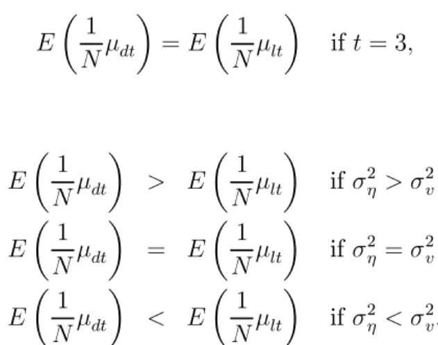
E¡N1µdt ¢ E¡1 Nµlt ¢ = ¡ σ2 v+ (t−3)σ2η ¢ (t−2)σ2 v = 1 t−2 µ 1 + (t−3)σ 2 η σ2 v ¶ .
Therefore E µ 1 Nµdt ¶ =E µ 1 Nµlt ¶ if t = 3, and for t >3 E µ 1 Nµdt ¶ > E µ 1 Nµlt ¶ if σ2η > σ2v E µ 1 Nµdt ¶ = E µ 1 Nµlt ¶ if σ2η =σ2v E µ 1 Nµdt ¶ < E µ 1 Nµlt ¶ if σ2η < σ2v.
Figure1graphs the values ofE¡N1µdt ¢
andE¡N1µdl ¢
as a function ofα fort= 6and various values of σ2η σ2 v = ©1 4,1,4 ª
. The values of the concentration parameters decrease with increasingα. The concentration parameter for the LEV model is much more sensitive to the value of the variance ratio σ2η
σ2
v than the concentration parameter of the DIF model.
Figure1. E¡1 Nµ ¢ as a function of α, t= 6and σ2η σv = ©1 4,1,4 ª .
4.1
Discussion
The fact that the concentration parameters are the same for the IV estimators based on the DIF or LEV moment conditions fort= 3and fort >3whenσ2
η =σ2v seems contrary to the findings in Monte Carlo studies, see e.g. Blundell and Bond (1998) and Blundell, Bond and Windmeijer (2000) who use a covariance stationary design with σ2η =σ2v = 1,
and wherebαloutperformsαbdin terms of bias and rmse, especially when the series become more persistent, i.e. when α gets larger. The identification problem is apparent in the DIF model, where the reduced form parameters approach zero whenαapproaches1. This is in sharp contrast to the reduced form parameters in the LEV model that approach 12 whenαapproaches1. This was the argument used by Blundell and Bond (1998) to assert the strength of the LEV moment conditions for the estimation of α for larger values of
α.
There are two questions to be addressed. Firstly, why are the behaviours of the two estimators so different in terms of bias and rmse when they have the same expected concentration parameter? Secondly, how does the weak instrument problem in the LEV model manifest itself?
To answer thefirst question one has to realise that the structural models are different for DIF and LEV, with different endogeneity problems and therefore different biases of the OLS estimator in the two equations. For the DIF model
∆yit=α∆yi,t−1+∆uit,
the OLS estimator for the cross-section at timet is given by
b αdOLS =α+ ∆y0 t−1∆ut ∆y0 t−1∆yt−1 ,
and the limiting bias of the OLS estimator is, again assuming covariance stationarity,
plim (αbdOLS−α) =−
1 +α
2 .
For the LEV model
yit=αyi,t−1+ηi+vit,
the OLS estimator is given by
b αlOLS =α+ y0 t−1ut y0 t−1yt−1 ,
and the limiting bias of the OLS estimator is given by plim (bαlOLS −α) = (1−α) σ2 η σ2 v σ2 η σ2 v + 1−α 1+α
which reduces toplim (bαlOLS −α) = (1−α2)/2when σ2η =σ2v.
The asymptotic absolute bias ofαblOLS is therefore (much) smaller than that of bαdOLS for high values ofα. Stock and Yogo (2005) relate the value of the concentration para-meter to the absolute bias of the 2SLS estimator, relative to the absolute bias of the OLS estimator. When the concentration parameters are the same, we expect therefore that the relative biases are the same for the DIF and LEV 2SLS estimators. But the absolute bias of the LEV 2SLS estimator will then be smaller than that of the DIF estimator. From the results of Stock and Yogo (2005) we further expect the Wald test statistics to behave similarly when testing parameter restrictions. When the concentration parameters are small there will be significant size distortions.
4.2
System Estimator
For the cross-section at timet the SYS estimator combines the moment conditions of the DIF and LEV estimators. The OLS estimator in the SYS "model"
µ ∆yt yt ¶ =α µ ∆yt−1 yt−1 ¶ + µ ∆ut ut ¶ (15) is given by b αsOLS = ¡ ∆yt0∆yt+yt0−1yt−1 ¢−1¡ ∆y0t−1∆yt+yt0−1yt ¢ and is clearly a weighted average of the DIF and LEV OLS estimators
b
αsOLS =eγbαdOLS+ (1−eγ)αblOLS
where e γ = ∆y 0 t∆yt ∆y0 t∆yt+y0t−1yt−1
and plimeγ = 1−α 2 + 12σ2η σ2 v 1+α 1−α .
The bias of the OLS estimator will therefore behave like the bias of the LEV OLS estimator when α → 1 and/or σ2
η/σ2v → ∞, as γe → 0 in these cases. The asymptotic bias of bαsOLS is given by
plim (bαsOLS −α) = (1−α2)³α −1 + σ2η σ2 v ´ (3−2α) (1−α) + σ2η σ2 v(1 +α) .
Figure 2 shows the asymptotic biases of the DIF, LEV and SYS OLS estimators as a function of α for different values of σ2
η/σ2v = ©1
4,1,4 ª
. It is clear from this picture that the LEV and SYS OLS biases are much smaller than the DIF OLS bias for higher values of α.
Figure 2. Asymptotic biases of OLS estimators, σ2 η/σ2v =
©1 4,1,4
ª .
The SYS 2SLS estimator for cross sectiont is also a weighted average of the DIF and LEV cross sectional 2SLS estimators
b αs =eδαbd+ ³ 1−eδ´bαl where eδ = πb 0 dZ 0 dZdbπd b π0dZ 0 dZdπbd+bπ0lZ 0 lZlbπl ,
see also Blundell, Bond and Windmeijer (2000), with plimeδ= E ¡1 Nµd ¢ E¡N1µd¢+ σ2l σ2 dE ¡1 Nµl ¢ and again eδ → 0 if α → 1 and/or σ2
η/σ2v → ∞. Clearly, the absolute bias of the SYS 2SLS estimator will be smaller than the maximum of the absolute biases of the DIF and LEV 2SLS estimators.
Combining the results of the OLS biases, values of the concentration parameters in the DIF and LEV models and relative weights on the DIF and LEV moment conditions in the SYS 2SLS estimator, we expect the absolute bias of the SYS estimator to be small for large values ofα, but that this bias is an increasing function of σ2η
σ2
v. This happens because
the bias of the LEV OLS estimator is an increasing function of σ2η
σ2
v, the LEV concentration
parameter a decreasing function of σ2η
σ2
v, and the weight
³
1−eδ´an increasing function in σ2
η
σ2
v, implying that more weight will be given to the LEV moment conditions.
Clearly, the SYS 2SLS estimator is not efficient as there is heteroskedasticity and correlation between the errors in model (15). We will focus on the 2SLS estimator here in the cross-section analysis and consider the efficient 2-step GMM estimator below when considering the full panel data analysis.
4.3
Some Monte Carlo Results
To investigate the finite sample behaviour of the estimators and Wald test statistics we conduct the following Monte Carlo experiment. We compute the OLS and 2SLS estimators for LEV, DIF and SYS for the cross sectiont = 6for the model specification
yi1 = ηi 1−α +εi; yit = αyi,t−1+ηi+vit; εi ∼N µ 0, σ 2 v 1−α2 ¶ ; ηi ∼N¡0, σ2η¢; vit ∼N ¡ 0, σ2v¢,
for sample sizeN = 200; σ2v = 1, and different values ofα={0.4,0.8}andσ2η = ©1
4,1,4 ª
. There are 4 instruments for the DIF and LEV 2SLS estimators, whereas the SYS 2SLS estimator is in this cross-sectional case based on the 8 combined moment conditions. Tables 1 and 2 present the estimation results for 10,000 Monte Carlo replications for
α= 0.4 andα= 0.8 respectively.
The results in Tables 1 and 2 confirm the findings and conjectures stated in the previous sections. The DIF OLS (absolute) bias is larger than the LEV OLS bias in all cases, especially when the series are more persistent withα= 0.8. The relative biases of the DIF 2SLS and LEV estimators are, however, the same whenσ2
η =σ2v. These relative biases are equal to 0.052 and 0.057 respectively whenα= 0.4, in which case the expected concentration parameters are equal to 46.75. The relative biases are larger, 0.310 and 0.312 respectively when α = 0.8. For this case the expected concentration parameters are much smaller and equal to 6.35, which corresponds to a first-stage F-statistic of
6.35/4 = 1.58.
The relative bias of the DIF 2SLS estimator does not vary much with the different values of σ2η when α = 0.4, whereas that of the LEV 2SLS estimator does. It is only 0.029 when σ2
η = 14, but increases to 0.169 when σ 2
η = 4. These are exactly in line with the larger variation in the values of the expected concentration parameter for the LEV model. They are132.7 when σ2
η = 1
4 and 13.0 when σ 2
η = 4, compared to 58.1 and 42.3 respectively for the DIF model. The absolute bias of the DIF 2SLS estimator is smaller than that of the LEV 2SLS one whenσ2
η = 4, but larger in the other cases.
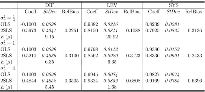
Whenα= 0.8, there is a similar pattern to the results of the relative biases. For the LEV 2SLS model it now decreases to 0.11whenσ2η = 14, with the expected concentration parameter equal to 20.9. It increases to 0.68 whenσ2η = 4and the expected concentration parameter is only 1.68. As explained before, we see that the weak instrument problem for the LEV moment conditions, givenα, becomes more severe with increasingσ2
both the OLS bias and the relative bias increase with increasingσ2η, so does the absolute bias of the 2SLS estimator. Whenα= 0.8, the absolute bias of the LEV 2SLS estimator ranges from 0.015 whenσ2
η = 1
4 to 0.132 whenσ 2 η = 4.
The SYS 2SLS estimator has a slightly smaller relative bias than the DIF and LEV ones when σ2
η = σ2v. It is 0.03 when α = 0.4 and 0.24 when α= 0.8. Unlike the results for the LEV 2SLS estimator, the relative bias actually increases when σ2
η = 1
4, although the absolute bias is quite small, especially whenα= 0.8. The relative bias is quite large in that case because the bias of the SYS OLS estimator is very small. Whenσ2η = 4 the relative and absolute biases of the SYS 2SLS estimator are similar to that of the LEV 2SLS estimator, albeit slightly smaller.
Table1. Cross Section Estimation Results forα = 0.4,N = 200, t= 6 andσ2 v = 1
DIF LEV SYS
Coeff StDev RelBias Coeff StDev RelBias Coeff StDev RelBias
σ2 η = 14 OLS -0.3005 0.0670 0.6208 0.0555 0.2243 0.0566 2SLS 0.3698 0.1734 0.0431 0.4064 0.0915 0.0289 0.3890 0.0810 0.0627 E(µ) 58.06 132.7 σ2 η = 1 OLS -0.3005 0.0670 0.8196 0.0407 0.5230 0.0491 2SLS 0.3637 0.1892 0.0518 0.4240 0.1131 0.0572 0.4038 0.0953 0.0306 E(µ) 46.75 46.75 σ2 η = 4 OLS -0.3005 0.0670 0.9416 0.0239 0.8118 0.0292 2SLS 0.3604 0.1973 0.0566 0.4917 0.1565 0.1694 0.4622 0.1223 0.1511 E(µ) 42.31 13.02
Table 2. Cross Section Estimation Results forα = 0.8,N = 200, t= 6 andσ2v = 1
DIF LEV SYS
Coeff StDev RelBias Coeff StDev RelBias Coeff StDev RelBias
σ2 η = 14 OLS -0.1003 0.0699 0.9382 0.0246 0.8239 0.0281 2SLS 0.5973 0.4041 0.2251 0.8150 0.0841 0.1088 0.7925 0.0825 0.3136 E(µ) 9.15 20.92 σ2 η = 1 OLS -0.1003 0.0699 0.9798 0.0142 0.9380 0.0153 2SLS 0.5210 0.4636 0.3100 0.8562 0.0920 0.3123 0.8336 0.0901 0.2433 E(µ) 6.35 6.35 σ2 η = 4 OLS -0.1003 0.0699 0.9945 0.0074 0.9827 0.0074 2SLS 0.4844 0.4852 0.3505 0.9324 0.0852 0.6808 0.9169 0.0785 0.6396 E(µ) 5.45 1.68
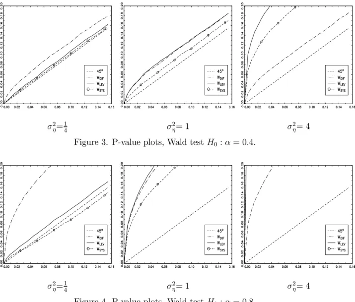
Figures 3 and 4 display p-value plots for the Wald test for testing H0 :α = α0 with
α0 the true parameter value. When σ2η = σ2v = 1, the size properties of the Wald tests based on the DIF and LEV 2SLS estimates are virtually identical, which is as expected as the concentration parameters are equal in expectation. It is also clear that when
α= 0.8, the size properties of the Wald tests are very poor, with a large overrejection of the null reflecting the low value of the concentration parameters. The size properties of the Wald test based on the SYS 2SLS estimation results are better than those based on the DIF and LEV 2SLS results, but again very poor when α = 0.8. When σ2η = 14 the size properties of the Wald tests based on the LEV and SYS 2SLS estimation results are quite good, even when α= 0.8, whereas they are very poor when σ2
η = 4. The Wald test results based on the DIF 2SLS estimates are not very sensitive to the value ofσ2
η. These results are again in line with expectation given the results of the previous section.
σ2 η= 1 4 σ 2 η= 1 σ2η= 4
Figure 3. P-value plots, Wald test H0 :α= 0.4.
σ2 η= 1 4 σ 2 η= 1 σ2η= 4
Figure 4. P-value plots, Wald test H0 :α= 0.8.
4.4
Mean Stationarity Only
In all the derivations so far we assumed covariance stationarity of the initial condition. When we assume mean stationarity only, i.e.
yi1 =
ηi
1−α +εi
withE(ε2i) =σ2ε, we show in the Appendix that fort= 3
E µ 1 Nµl3 ¶ > E µ 1 Nµd3 ¶ if σ2ε < σ 2 v 1−α2 E µ 1 Nµl3 ¶ < E µ 1 Nµd3 ¶ if σ2ε > σ 2 v 1−α2,
so that, when t = 3, the expected concentration parameter for the LEV model is larger than that of the DIF model when the variance of the initial condition is smaller than the covariance stationary level and vice versa.
5
Panel Data Analysis
The concept of the concentration parameter and its relationship to relative bias and size distortion of the Wald test does not readily extend itself to general GMM estimation, see e.g. Stock and Wright (2000) and Han and Phillips (2006). Estimation of the panel AR(1) model by 2SLS, using all available time periods and the full set of sequential moment conditions for the DIF and SYS models (6) and (12) will result in a weighted average of the period specific 2SLS estimates. Weighting by the efficient weight matrix will lead to different results, but we expect the weak instrument issues as documented in the previous section for the DIF and LEV cross-sectional estimates to carry over to the linear GMM estimation. This is indeed confirmed by our Monte Carlo results presented here.
Table 3 presents Monte Carlo estimation results for the AR(1) model with normally distributed ηi andvi, withN = 200,T = 6, α= 0.8 andσ2v = 1, varyingσ2η =
©1 4,1,4
ª . We present 2SLS and1-step and 2-step GMM estimation results. We use for the initial weight matrix for the 1-step GMM DIF estimator WN = PNi=1Zdi0 AZdi where A is a
(T −2) square matrix that has 2s on the main diagonal, −1s on the first subdiagonals, and zeros elsewhere. This is the efficient weight matrix for the DIF moment conditions when the vit are homoskedastic and not serially correlated, as is the case here. For the
1-step GMM SYS estimator we use the commonly used initial weight matrix WN = PN
i=1Zsi0 HZsi where H is a2 (T −2) square matrix
H = · A 0 0 IT−2 ¸ ,
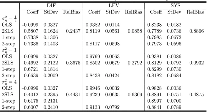
The pattern of results for the 2SLS estimates is quite similar to that found for the
t = 6 cross-section as reported in Table 2. The DIF 2SLS estimator displays somewhat larger relative biases, whereas the LEV 2SLS estimator has smaller relative biases than in the cross-section. SYS has smaller relative and absolute biases atσ2
η = 1 andσ2η = 4, but the direction of the biases remain the same.
Use of the efficient initial weight matrix reduces the bias of the 1-step GMM DIF estimator significantly. This is due to the fact that the comparison bias is now no longer the OLS bias in the first differenced model, but the bias of the within groups estimator, which is smaller. There is no clear pattern to the bias of the SYS one- and two-step GMM estimators in comparison to the 2SLS estimator.
Table 3. Panel Data Estimation Results, N = 200, T = 6, α= 0.8 andσ2v = 1
DIF LEV SYS
Coeff StDev RelBias Coeff StDev RelBias Coeff StDev RelBias
σ2 η = 14 OLS -0.0999 0.0327 0.9382 0.0114 0.8238 0.0182 2SLS 0.5807 0.1624 0.2437 0.8119 0.0561 0.0858 0.7789 0.0736 0.8866 1-step 0.7338 0.1306 0.7983 0.0672 2-step 0.7336 0.1403 0.8117 0.0598 0.7973 0.0596 σ2 η = 1 OLS -0.0999 0.0327 0.9799 0.0063 0.9381 0.0086 2SLS 0.4692 0.2122 0.3675 0.8502 0.0679 0.2792 0.8129 0.0792 0.0932 1-step 0.6721 0.1814 0.8299 0.0730 2-step 0.6639 0.2009 0.8438 0.0424 0.8182 0.0684 σ2 η = 4 OLS -0.0999 0.0327 0.9946 0.0032 0.9828 0.0036 2SLS 0.4012 0.2395 0.4431 0.9239 0.0635 0.6369 0.8891 0.0751 0.4875 1-step 0.6175 0.2131 0.8997 0.0700 2-step 0.6007 0.2410 0.9133 0.0792 0.8841 0.0789
Figure 5 displays the p-value plots of the Wald tests for testing H0 : α = 0.8 based on the DIF and SYS GMM estimation results, where the Wald tests based on the 2-step GMM results use the Windmeijer (2005) corrected variance estimates. The pattern of size properties is very similar to that for the cross-section analysis. The Wald test
based on the SYS GMM estimation results has better size properties than that based on the DIF GMM estimation results whenσ2
η = 14, especially for the 1-step SYS GMM estimator. The size behaviours are very similar when σ2
η = 1, but the SYS Wald tests size properties are much worse than that of the DIF Wald tests when σ2
η = 4.
σ2η = 14 σ2η = 1 σ2η = 4
Figure 5. P-value plots, Wald test H0 :α= 0.8.
6
Conclusions
We have shown that the concentration parameters in the reduced forms of the DIF and LEV cross-sectional models are the same in expectation when the variances of the unobserved heterogeneity (σ2
η) and idiosyncratic errors (σ2v) are the same in the covariance stationary AR(1) model. The LEV concentration parameter is smaller than the DIF one if σ2η > σ2v and it is larger if σ2η < σ2v. Therefore, the well-understood weak instrument problem in the DIF model also applies to the LEV model, especially when σ2η ≥ σ2v, with both concentration parameters decreasing in value with increasing persistence of the data series. The weak instrument problem does manifest itself in the magnitude of the bias of 2SLS relative to that of OLS, which we show are equal for DIF and LEV when σ2
η = σ2v. The LEV 2SLS estimator has a smaller finite sample performance in terms of bias though, because the OLS bias of the LEV structural equation is smaller
than that of DIF, especially when the series are persistent. The weak instrument problem further manifests itself in poor performances of the Wald tests, which we show to have the same size distortions in the DIF and LEV models whenσ2
η =σ2v. We show that these properties generalise to the system GMM estimator.
Having established this potential weak instrument problem for the system GMM estimator, for inference one should therefore consider use of testing procedures that are robust to the weak instruments problem. The Kleibergen (2005) Lagrange Multiplier test and his GMM extension of the Conditional Likelihood Ratio test of Moreira (2003) are possible candidates, as is the Stock and Wright (2000) GMM version of the Anderson-Rubin statistic. Newey and Windmeijer (2007) show that the behaviours of these test statistics are not only robust to weak instrument asymptotics, they are also robust to many weak instrument asymptotics, where the number of instruments grow with the sample size, but with the model bounded away from non-identification. Newey and Windmeijer (2007) also propose use of the continuous updated GMM estimator (CUE, Hansen, Heaton and Yaron (1996)) with a new variance estimator that is valid under many weak instrument asymptotics. They show that the Wald test using the CUE estimation results and their proposed variance estimator performs well in a static panel data model estimated infirst differences. As the number of potential instruments in this panel data setting grow quite rapidly with the time dimension of the panel, this may be a sensible approach also for the system moment conditions.
As a final remark, the direction of the biases of the DIF (downward) and LEV (up-ward) GMM estimators in the AR(1) panel data model are quite specific to this model specification. In different models these biases may be different and the SYS GMM esti-mator may have a larger absolute bias than the DIF GMM estiesti-mator. For example in
the static panel data model
yit = xitβ+ηi+vit
xit = ρxi,t−1+γηi+δvit+wit
the DIF GMM estimator may have a smaller finite sample bias than the SYS GMM estimator when thexit series are persistent, but |δ| is small and |γ| is large, as then the endogeneity problem and OLS bias in the DIF model may be less than that of the LEV model.
References
[1] Arellano, M. and S. Bond (1991), Some Tests of Specification for Panel Data: Monte Carlo Evidence and an Application to Employment Equations, Review of Economic Studies 58, 277-298.
[2] Arellano, M. and O. Bover (1995), Another Look at the Instrumental Variable Es-timation of Error-Components Models, Journal of Econometrics 68, 29-51.
[3] Blundell, R. and S. Bond, 1998, Initial Conditions and Moment Restrictions in Dynamic Panel Data Models, Journal of Econometrics 87, 115-143.
[4] Blundell, R.W., S.R. Bond and F. Windmeijer (2000), Estimation in Dynamic Panel Data Models: Improving on the Performance of the Standard GMM Estimator’, in B. Baltagi (ed.), Nonstationary Panels, Panel Cointegration, and Dynamic Panels, Advances in Econometrics 15, JAI Press, Elsevier Science.
[5] Bond, S.R., A. Hoeffler and J. Temple (2001). GMM Estimation of Empirical Growth Models, Working Paper, University of Oxford.
[6] Bond, S.R. and F. Windmeijer (2005), Reliable Inference for GMM Estimators? Fi-nite Sample Properties of Alternative Test Procedures in Linear Panel Data Models,
Econometrics Reviews 24, 1-37.
[7] Bound, J., D.A. Jaeger and R.M. Baker (1995), Problems with Instrumental Vari-ables Estimation when the Correlation between the Instruments and the Endogenous Explanatory Variable is Weak, Journal of the American Statistical Association 90, 443-450.
[8] Bun, M.J.G. and J.F. Kiviet (2006), The Effects of Dynamic Feedbacks on LS and MM Estimator Accuracy in Panel Data Models,Journal of Econometrics 132, 409-444.
[9] Griffith, R., R. Harrison and J. Van Reenen (2006), How Special is the Special Relationship? Using the Impact of U.S. R&D Spillovers on U.K. Firms as a Test of Technology Sourcing,The American Economic Review 96, 1859-1875.
[10] Han, C. and P.C.B. Phillips (2006), GMM with Many Moment Conditions, Econo-metrica 74, 147-192.
[11] Hansen, L.P., J. Heaton and A. Yaron (1996), Finite-Sample Properties of Some Alternative GMM Estimators,Journal of Business and Economic Statistics 14, 262-280.
[12] Hayakawa, K. (2005), Small Sample Bias Properties of the System GMM Estimator in Dynamic Panel Data Models, Hi-Stat Discussion Paper Series d05-82, Institute of Economic Research, Hitotsubashi University.
[13] Kleibergen, F. (2005) Testing Parameters in GMM Without Assuming They are Identified, Econometrica 73, 1103-1123.
[14] Levine, R., L. Norman and T. Beck (2000), Financial Intermediation and Growth: Causality and Causes,Journal of Monetary Economics 46, 31-77.
[15] Levinsohn, J. and A. Petrin (2003), Estimating Production Functions Using Inputs to Control for Unobservables, Review of Economic Studies 70, 317-341.
[16] Moreira, M. (2003), A Conditional Likelihood Ratio Test for Structural Models,
Econometrica 71, 1027-1048.
[17] Newey, W.K. and F. Windmeijer (2007), GMM with Many Weak Moment Condi-tions, working paper, MIT.
[18] Picone, G.A., F. Sloan and J.G. Trogdon (2004), The Effect of the Tobacco Settle-ment and Smoking Bans on Alcohol Consumption,Health Economics 13,1063-1080.
[19] Ridder, G. and T. Wansbeek (1990), Dynamic Models for Panel Data, in F. van der Ploeg (ed.), Advanced Lectures in Quantitative Economics, Academic Press.
[20] Rothenberg, T.J. (1984), Approximating the Distributions of Econometric Estima-tors and Test Statistics, in Z. Griliches and M.D. Intriligator (eds.), Handbook of Econometrics, Vol. II, North Holland, 881-935.
[21] Staiger, D. and J.H. Stock (1997), Instrumental Variables Regression with Weak Instruments, Econometrica 65, 557-586.
[22] Stock, J.H. and J.H. Wright (2000), GMM with Weak Identification,Econometrica
68, 1055-1096.
[23] Stock, J.H., J.H. Wright and M. Yogo (2002), A Survey of Weak Instruments and Weak Identification in Generalized Method of Moments, Journal of Business & Economic Statistics, 518-529.
[24] Stock, J.H. and M. Yogo (2005), Testing for Weak Instruments in Linear IV Re-gression, in D.W.K. Andrews and J.H. Stock (eds.),Identification and Inference for Econometric Models, Essays in Honor of Thomas Rothenberg, Cambridge University Press.
[25] Windmeijer, F. (2005), A Finite Sample Correction for the variance of Linear Effi -cient Two-Step GMM Estimators,Journal of Econometrics 126, 25-517.
7
Appendix
7.1
Concentration parameters in cross-section analysis
The model infirst differences for the cross-section at time t is given by
∆yit = α∆yi,t−1+∆uit ∆yi,t−1 = yit−20πdt+dti,t−1.
For the general expression of the expected value of the concentration parameter divided byN we get E µ 1 Nµdt ¶ = π 0 dtE ¡ yti−2y t−20 i ¢ πdt σ2 dt but as πdt = £ E¡yit−2yit−20¢¤−1E¡yit−2∆yi,t−1 ¢ and σ2dt =E ³¡ ∆yi,t−1−yti−20πdt ¢2´ we get E µ 1 Nµdt ¶ = ¡ E¡yti−2∆yi,t−1 ¢¢0£ E¡yti−2yit−20¢¤−1E¡yit−2∆yi,t−1 ¢ E¡∆y2 i,t−1 ¢ −¡E¡yti−2∆yi,t−1 ¢¢0£ E¡yti−2yit−20¢¤−1E¡yit−2∆yi,t−1 ¢.
Under covariance stationarity E¡yit−2yti−20 ¢ = σ 2 η (1−α)2ιt−2ι 0 t−2+ σ2v 1−α2Gt−2 where Gt−2 = 1 α · · · αt−3 α 1 ... .. . . .. α αt−3 · · · α 1 .
The inverse of E¡yit−2yit−20¢ is given by (see e.g. Ridder and Wansbeek (1990)) £ E¡yit−2yit−20¢¤−1 = 1 σ2 v " R0t−2Rt−2− σ2 ηht−2h0t−2 σ2 v+σ2η ¡ t−3 + 1+α 1−α ¢ # where Rt−2 = 1 −α 0 0 0 1 −α . .. ... 1 −α 0 0 √1−α2 ; ht−2 = (1−α)ιt−2+α(e1 +et−2)
and ej is the j-th unit vector of ordert−2. We further have that
E¡yit−2∆yi,t−1 ¢ =− σ 2 v 1 +αgt−2 where gt−2 = αt−3 .. . α 1 . As Rt−2gt−2 = 0 .. . 0 √ 1−α2 ; h 0 t−2gt−2 = 1 +α and so ¡ E¡yit−1∆yi,t−1 ¢¢0£ E¡yti−2y t−20 i ¢¤−1 E¡yti−2∆yi,t−1 ¢ = σ 2 v (1 +α)2 à 1−α2− σ 2 η(1 +α) 2 σ2 v+σ2η ¡ t−3 + 1+α 1−α ¢ ! .
Further
E¡∆y2i,t−1¢= 2σ
2 v
1 +α.
Combining these results in
E µ 1 Nµdt ¶ = σ2v (1+α)2 µ 1−α2 − σ2η(1+α)2 σ2 v+σ2η(t−3+1+1−αα) ¶ 2σ2 v 1+α − σ2 v (1+α)2 µ 1−α2− σ2η(1+α)2 σ2 v+σ2η(t−3+1+1−αα) ¶ = 1−α2 − σ2η(1+α)2 σ2 v+σ2η(t−3+1+1−αα) 2 (1 +α)− µ 1−α2− σ2η(1+α)2 σ2 v+σ2η(t−3+1+1−αα) ¶ = (1−α 2)¡σ2 v +σ2η ¡ t−3 + 1+1−αα¢¢−σ2 η(1 +α) 2 (1 +α)2¡σ2 v +σ2η ¡ t−3 + 1+1−αα¢¢+σ2 η(1 +α) 2 = (1−α) ¡ σ2 v + (t−3)σ2η ¢ (1 +α)¡σ2 v+σ2η ¡ t−2 + 1+1−αα¢¢ = (1−α) 2¡ σ2v + (t−3)σ2η ¢ (1−α2)σ2 v+ ((t−1)−(t−3)α) (1 +α)σ2η .
For the model in levels we have for the cross-section at time t
yit = αyi,t−1 +ηi+vit
yi,t−1 = ∆yit−10πlt+lti,t−1 and the expected concentration parameter is given by
E µ 1 Nµlt ¶ = ¡ E¡yi,t−1∆yit−1 ¢¢0£ E¡∆yit−1∆y t−10 i ¢¤−1 E¡yi,t−1∆yit−1 ¢ E¡y2 i,t−1 ¢ −¡E¡yi,t−1∆yit−1 ¢¢0£ E¡∆yit−1∆yit−10¢¤−1E¡yi,t−1∆yit−1 ¢.
Again, under covariance stationarity, we have that
E¡∆yit−1∆yit−10¢= σ 2 v 1 +α 2 α−1 α(α−1) · · · αt−4(α−1) α−1 2 α−1 · · · αt−5(α−1) α(α−1) α−1 2 . .. ... .. . . .. . .. . .. α−1 αt−4(α −1) · · · α(α−1) α−1 2
and E¡yi,t−1∆yit−1 ¢ = σ 2 v 1 +α αt−3 .. . α 1 .
It then follows that
E¡yi,t−1∆yit−1 ¢0£ E¡∆yit−1∆yti−10¢¤−1E¡yi,t−1∆yti−1 ¢ = (t−2)σ 2 v (1 +α) ((t−1)−(t−3)α). As E¡yi,t2−1¢ = σ 2 η (1−α)2 + σ2v 1−α2 we get that E µ 1 Nµlt ¶ = (t−2)σ2 v (1+α)((t−1)−(t−3)α) σ2 η (1−α)2 + σ2 v 1−α2 − (t−2)σ2 v (1+α)((t−1)−(t−3)α) = (t−2)σ 2 v (1 +α) ((t−1)−(t−3)α)³ σ2η (1−α)2 + σ2 v 1−α2 ´ −(t−2)σ2 v = (t−2) (1−α) 2 σ2 v ((t−1)−(t−3)α)¡(1 +α)σ2 η + (1−α)σ2v ¢ −(t−2) (1−α)2σ2 v = (t−2) (1−α) 2 σ2 v (1−α2)σ2 v+ ((t−1)−(t−3)α) (1 +α)σ2η
7.2
Mean stationarity only
We now relax the assumption of covariance stationarity, while maintaining mean station-arity, i.e. we specify the initial condition as
yi1 =
ηi
1−α +εi
withE[ε2i] =σ2ε.
Fort = 3, we get in this case
πd3 = E(y1∆y2) E(y2 1) =−(1−α)σ 2 ε σ2 η (1−α)2 +σ 2 ε =−(1−α)σ 2 ε σ2 y1
σ2d3 = E(∆y2)2−2πdE(y1∆y2) +π2d3E ¡ y12 ¢ = σ2v + (1−α)2σε2+πd3(1−α)σ2ε µd3 = π2 d3y10y1 σ2 d3 = π 2 d3 σ2 v + (1−α) 2 σ2 ε+πd3(1−α)σ2ε y10y1. E µ 1 Nµd3 ¶ = ³ (1−α)σ2ε σ2 y1 ´2 σ2 v+ (1−α) 2 σ2 ε− ((1−α)σ2 ε)2 σ2 y1 σ2y1 = ((1−α)σ2ε)2 σ2 y1 σ2 v+ (1−α) 2 σ2 ε− ((1−α)σ2 ε)2 σ2 y1
For the levels model we get
πl3 = E(y2∆y2) E¡(∆y2) 2¢ = σ 2 v−α(1−α)σ2ε σ2 v+ (1−α) 2 σ2 ε and σ2l3 = E ¡ y22¢−πl3E(y2∆y2) = σ 2 η (1−α)2 +σ 2 v+α 2σ2 ε− (σ2 v−α(1−α)σ2ε) 2 σ2 v+ (1−α) 2 σ2 ε .
The concentration parameter is therefore given by
µl3 = π2l3∆y20∆y2 σ2 l3 = ³σ2 v−α(1−α)σ2ε σ2 v+(1−α) 2σ2 ε ´2 σ2 η (1−α)2 +σ 2 v+α2σ2ε− (σ2 v−α(1−α)σ2ε) 2 σ2 v+(1−α)2σ2ε ∆y20∆y2
and so E µ 1 Nµl3 ¶ = (σ2 v−α(1−α)σ2ε) 2 σ2 v+(1−α) 2σ2 ε σ2 η (1−α)2 +σ 2 v +α2σ2ε− (σ2 v−α(1−α)σ2ε) 2 σ2 v+(1−α)2σ2ε .
Calculating these expectations shows that E¡N1µl3 ¢ > E¡N1µd3 ¢ if σ2ε < σ2 v 1−α2 and E¡1 Nµl3 ¢ < E¡1 Nµd3 ¢ if σ2 ε > σ2 v
1−α2, i.e. the expected concentration parameter in the levels model is larger than that of the differenced model if the variance of the initial condition is smaller than the covariance stationary level and vice versa.