Line Based Multi-Range Asymmetric Conditional Random Field For Terrestrial Laser Scanning Data Classification

(1)

Line Based Multi-range Asymmetric Conditional Random

Field for Terrestrial Laser Scanning Data Classification

Chao Luo

A DISSERTATION SUBMITTED TO THE FACULTY OF GRADUATE STUDIES

IN PARTIAL FULFILLMENT OF THE REQUIREMENTS FOR THE DEGREE OF

DOCTOR OF PHILOSOPHY

GRADUATE PROGRAM IN EARTH AND SPACE SCIENCE

YORK UNIVERSITY

TORONTO, ONTARIO

DECEMBER, 2015

(2)

Abstract

Terrestrial Laser Scanning (TLS) is a ground-based, active imaging method that rapidly

acquires accurate, highly dense three-dimensional point cloud of object surfaces by laser

range finding. For fully utilizing its benefits, developing a robust method to classify

many objects of interests from huge amounts of laser point clouds is urgently required.

However, classifying massive TLS data faces many challenges, such as complex urban

scene, partial data acquisition from occlusion. To make an automatic, accurate and robust

TLS data classification, we present a line-based multi-range asymmetric Conditional

Random Field algorithm.

The first contribution is to propose a line-base TLS data classification method.

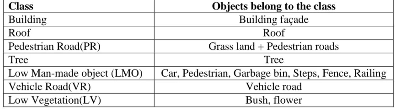
In this thesis, we are interested in seven classes: building, roof, pedestrian road (PR), tree,

low man-made object (LMO), vehicle road (VR), and low vegetation (LV). The

line-based classification is implemented in each scan profile, which follows the line profiling

nature of laser scanning mechanism. It is rather straightforward to extract lines in each

scan profile, and the appearance of scanned objects can be characterized using lines. Ten

conventional local classifiers are tested, including popular generative and discriminative

classifiers, and experimental results validate that the line-based method can achieve

satisfying classification performance. However, local classifiers implement labeling task

on individual line independently of its neighborhood, the inference of which often suffers

(3)

uses object context as post-classification to improve the performance of a local generative

classifier. The maCRF incorporates appearance, local smoothness constraint, and global

scene layout regularity together into a probabilistic graphical model. The local

smoothness enforces that lines in a local area to have the same class label, while scene

layout favours an asymmetric regularity of spatial arrangement between different object

classes within long-range, which is considered both in vertical (“above-bellow” relation)

and horizontal (“front-behind”) directions. The asymmetric regularity allows capturing

directional spatial arrangement between pairwise objects (e.g. it allows ground is lower

than building, not vice-versa). The third contribution is to extend the maCRF model by

adding across scan profile context, which is called Across scan profile Multi-range

Asymmetric Conditional Random Field (amaCRF) model. Due to the sweeping nature of

laser scanning, the sequentially acquired TLS data has strong spatial dependency, and the

across scan profile context can provide more contextual information. The final

contribution is to propose a sequential classification strategy. Along the sweeping

direction of laser scanning, amaCRF models were sequentially constructed. By

dynamically updating posterior probability of common scan profiles, contextual

information propagates through adjacent scan profiles.

The proposed methods are finally evaluated using datasets collected at two

different sites, York Village and York Blvd. And the experimental results validated the

advantage using multi-range contexts and sequential processing. As line extraction is

implemented in each scan profile, the line-based method has great potential on real-time

(4)

algorithm in a real-time environment is not available. Thus we simulate the line-based

(5)

Acknowledgements

I would like to extend my sincere gratitude to all of the people who supported and

helped me in the past six and half years.

At first, a very special word of appreciation gives to Dr. Gunho Sohn, my

supervisor, for his clear guidance, insightful suggestions, and challenging discussions that

I finished my PhD research on Machine Learning topic with a total different academic

background, Geographic Information System. His continuous encouragement and

supports created a stimulating academic environment that I appreciated.

I would like to thank Dr. Costas Armenakis (York University, GeoICT), and Dr.

James Elder (York University, GeoICT), the supervision committee members, for their

scientific suggestions, valuable advices, and encouragements which significantly speed

up my research progress. Particular gratitude to Dr. James Elder, who opened the door of

statistical machine learning to me, and guided me to solve the real world problem using

probabilistic models. I also thank my previous supervisors (Master degree), Dr. Huayi

Wu (Wuhan Univeristy, China) and MS. Aihong Song (Wuhan Univeristy, China), for

their continuous encouragements and helps.

Many individuals have contributed in different ways to my PhD research. I would

like to appreciate Dr. Yooseok Jwa (GeoICT, York University) for helping me to design

the framework of object recognition from mobile railway laser scanning data; Dr.

Heungsik Kim (GeoICT, York University) for helping me to explore potential application

(6)

line extraction, feature extraction; Mr. Jaewook Jung (GeoICT, York University) for

helping me to develop features and providing me visualization tool of TLS data; and Dr.

Mojgan Jadidi (GeoICT, York University), who gave me many suggestions on thesis

writing.

I wish to thank GEOmaticsfor Informed DEcisions (GEOIDE), Ontario Centres of

Excellence (OCE), Natural Sciences and Engineering Research Council of Canada

(NSERC) Discovery, Hyundai, and China Scholarship Council (CSC) for arranging the

financial support for this PhD research. Thank all my research partners from GeoICT,

Langyue Wang and Ravi Persad, and partners from CVR at York University, Eduardo

Corral-Soto and Ron Tal. Warm thanks to all other student members and visiting scholars

at GeoICT of York University, who helped me in my research, such as Dr. Yawen Liu,

Dr. Jili Li, Dr. Connie Ko, Dr. Junjie Zhang, Julien Lee-Chee-Ming.

Finally, I deeply thank my parents, Guixian Chen and Fuhua Luo, for their

endless love and continuous encouragement. They gave me support through their

(7)

Table of

List of Tables

Table 2.1: Technical specifications of RIEGL LMS Z-390i ... 19

Table 3.1: Object categorization of experimental dataset. ... 74

Table 3.2: Number of laser point, scan profile, line segment in York Village dataset. .... 75

Table 3.3: Confusion matrix of GMM classifier of data YV2. ... 79

Table 3.4: Confusion matrix of SVM classifier of data YV2. ... 79

Table 3.5: Precision of each class in ten classifiers. ... 82

Table 3.6: Recall of each class in ten classifiers. ... 82

Table 3.7: F1 score of each class in 10 classifiers. ... 83

Table 4.1: Total number of the spatial entities extracted from York Village datasets. .. 118

Table 4.2: Positive and negative transition from GMM to each CRF classifier. ... 125

Table 4.3: Test accuracy of GMM and the four CRF models. ... 129

Table 4.4: Confusion matrix of srCRF classifier on data YV2... 129

Table 4.5: Confusion matrix of lrCRF(V) classifier on data YV2. ... 130

Table 4.6: Confusion matrix of lrCRF(H) classifier on data YV2. ... 130

Table 4.7: Confusion matrix of maCRF classifier on data YV2... 130

Table 5.1: Total number of the spatial entities extracted from York Village datasets. .. 146

Table 5.2: Test Accuracy of sequential CRF Models. ... 149

Table 5.3: Test Accuracy of sequential CRF Models. ... 151

(13)

(14)

List of Figures

Figure 1.1: Examples of objects in terrestrial laser scanning data. ... 6

Figure 3.1: Examples of line extraction. ... 43

Figure 3.2: Post-processing using the Douglas–Peucker algorithm. ... 44

Figure 3.3: Neighborhood selection for context feature. ... 46

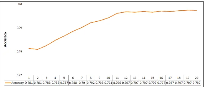
Figure 3.4: Averaged test accuracy over 5-fold cross validation. The value ... 59

Figure 3.5: Typical structure of ANN with three layers. ... 64

Figure 3.6: Averaged test accuracy over 5-fold cross validation as different minimum leaf size was selected. ... 68

Figure 3.7: Real scene of the York Village Data. ... 73

Figure 3.8: Classification result of GMM, SVM and ground truth. ... 77

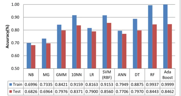
Figure 3.9: Averaged accuracy of ten classifiers. ... 80

Figure 4.1: Height distributions of seven classes... 87

Figure 4.2: Example of grid system and line-cell occupancy relations. ... 90

Figure 4.3: Multi-range neighborhood searching for each cell... 91

Figure 4.4: Prior and likelihood estimation for vertical interaction term. ... 101

Figure 4.5: Prior and likelihood estimation for horizontal interaction term. ... 104

Figure 4.6: Parameter learning of maCRF model using SGD algorithm on data YV1. . 119

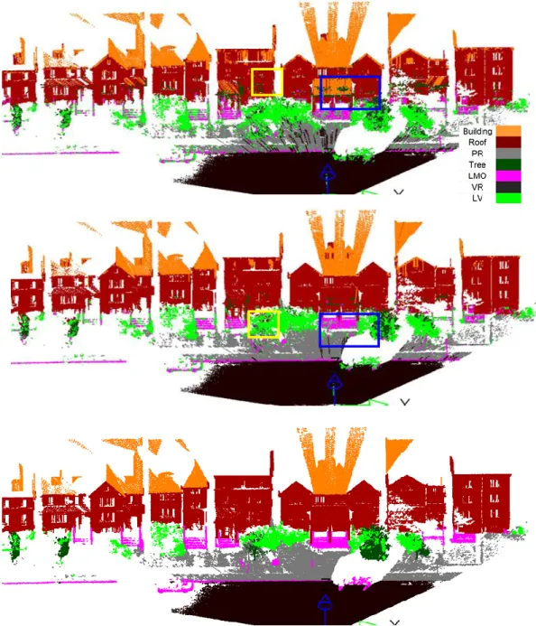
Figure 4.7: Classification result of the four CRFs of the data YV2. ... 121

(15)

Figure 4.10: Label transition from GMM to lrCRF(V). ... 126

Figure 4.11: Label transition from GMM to lrCRF(H). ... 127

Figure 4.12: Label transition from GMM to maCRF. ... 128

Figure 4.13: Precision of each class in five methods. ... 131

Figure 4.14: Recall of each class in five methods. ... 132

Figure 4.15: F1-Score of each class in five methods. ... 132

Figure 5.1: Across and along scan profile neighborhood. ... 138

Figure 5.2: Example of across/with scan profile multi-range graph. ... 139

Figure 5.3: Each amaCRF model is independent with each other. ... 142

Figure 5.4: Contextual information propagates through adjacent scan profiles. ... 144

Figure 5.5: Parameter learning of maCRF model on data YV1. ... 147

Figure 5.6: Classification result of the amaCRF model and sequential processing on the data YV2. ... 148

Figure 5.7: Parameter learning of the amaCRF model (SVM) on data YV1. …………150

Figure 5.8: Classification result of the SVM-based amaCRF model and sequential processing on the data YV2. ... 152

Figure 5.9: Surveying locations of York Blvd Dataset. ... 153

Figure 5.10: Classification results of the GMM and GMM-based amaCRF model with sequential processing on the data YB2. ... 155

Figure 5.11: Classification results of the SVM and SVM-based amaCRF model with sequential processing on the data YB2. ... 156

(16)

List of Abbreviations

AdaBoost Adaptive Boosting

ALS Airborne Laser Scanning

amaCRF Across scan profile Multi-range Asymmetric CRF

amaCRF+ Across scan profile Multi-range Asymmetric CRF with sequential

modeling

AMN Associative Markov network

ANN Artificial Neural Network

BP Belief Propagation

CART Classification And Regression Tree

CRF Conditional Random Field

DLG Digital Linear Graph

DOM Digital Ortho-image Model

DRM Digital Raster graph Model

DT Decision Tree

DTM Digital Terrain Model

EM Expectation Maximization

GLCM Gray-Level Co-occurrence Matrix

GMM Gaussian Mixture Model

(17)

IMU Inertial Measurement Unit

KNN K-Nearest Neighbor

LBP Loopy Belief Propagation

LiDAR Light Detection And Ranging

LLF Label Layout Filter

LMO Low Man-made Object

LOD Level of Detail

LR Logistic Regression

LV Low Vegetation

maCRF Multi-range Asymmetric CRF

MG Multivariate Gaussian

MLE Maximum Likelihood Estimation

MRF Markov Random Field

NB Naïve Bayes

PR Pedestrian Road

PS Phase Shift

RANSAC RANdom SAmple Consensus

RBF Radial Basis Function

RF Random Forest

SAMME Stagewise Additive Modeling using a Multi-class Exponential loss

function

(18)

SVM Support Vector Machine

TLS Terrestrial Laser Scanning

ToF Time-of-Flight

VR Vehicle Road

YV York Village

(19)

Chapter 1 Introduction

1.1 Problem Domain

1.1.1 Research Context

Municipal infrastructure refers to the fundamental facilities and systems that serve for the

public. Typical infrastructures include public buildings, transportation networks, bridges,

train/bus stations, education facilities, and hospital service, etc. Urbanization is the global

trend but the growing urban population brings challenges to municipal infrastructure

management. The “State of World Population 2014”, published by the United Nations

Population Fund (UNPF) that infrastructure shortage is a significant problem in

developing counties, especially those counties with fast population growth (UNPFA,

2014). Every day, new urban infrastructures are built while existing infrastructures

deteriorate, which poses a great demand for a sustainable management of municipal

infrastructure system, including construction, monitoring, and maintenance. A sustainable

municipal infrastructure management system enables city governments and related civic

service provides better services to the residences. Many governments have realized the

significance of a sustainable municipal infrastructure system, and have already taken

actions, such as Canada’s National Guide to Sustainable Municipal Infrastructure

(Boudreau and Brynildsen, 2003), and Singapore’s Future Cities Laboratory (FCL)

(20)

Risk assessment of infrastructures is one of the key elements of an infrastructure

management system. A 3D municipal infrastructure system can significantly reduce the

amount of cognitive effort, achieve a rapid response to plausible risks, and improve the

efficiency of the decision-making process (Kolbe et al. 2005, Zlatanova 2008). As one of

essential components of a municipal infrastructure system, 3D urban modeling is a

crucial work. Recently, 3D photo-realistic urban modeling, especially the 3D building

modeling has been attracting much attention from photogrammetric and computer vision

communities as there is an increasing demand for urban modeling applications, such as

urban planning, augmented reality and individual navigation. In 3D city visualization, the

same city object needs to be represented with different geometric complexities according

to users’ request. The Level of Detail (LOD) is usually used to describe the geometric

complexity of a 3D building, and allows the geometry of objects to be represented in

varying accuracies and details (Emgard and Zlatanova, 2008). Lee and Nevatia (2003)

proposed a hierarchical representation structure of 3D building models for 3D urban

reconstruction, in which the visualization quality of the building model increases when

LOD level upgrades. The coarsest LOD0 is essentially a 2.5D Digital Terrain Model

(DTM), and building models in LOD0 do not contain volume. In the LOD1 level,

building models are referred to as a block with flat roof structures. Both the outer facade

and roof of the buildings at LOD2 level can be represented with multiple faces.

Compared with lower-level models, LOD3 goes further by representing more detailed

facade geometries, such as wall, roof, door, window, sidewall, window sill .etc. The

(21)

For modeling realistic facilities, capturing digitized 3D geometric and textual

information is the first step. Photogrammetry has been and is still used as the main

method of collecting geo-spatial information of Earth surfaces over the past century.

Photogrammetry is passive remote sensing technology, and recovers 3D geometric and

photogrammetric information of real world by matching stereo pair images (Wolf et al.,

2000). Typical products of photogrammetry-based methods include digital elevation

model (DEM), digital ortho-image model (DOM), digital raster model (DRM), and

digital linear graph (DLG), which have been widely used for urban planning and

management. However, the main drawback of photogrammetric workflow is the low

efficiency in generating dense 3D coordinator from stereoscopic pictures and

somtimes-manual work (Alshawabkeh, Y., 2006). Recently, laser scanning compensates for this

drawback of photogrammetry by providing direct 3D data and has become a standard tool

for 3D data collection.

Airborne laser scanning (ALS) has been used for surveying and mapping since the

1980s, such as forest surveying (Rutzinger et al., 2008; Vehmas et al, 2009; Zhang and

Sohn, 2010; Kantola et al, 2013), digital surface modeling (Kraus and Pfeifer 1998).

Since ALS collects data from bird's-eye perspective, it can capture roofs of buildings

efficiently but only get part of building facade that is essential for LOD3 model. Due to

close range, high accuracy and cost-effectiveness, Terrestrial Laser Scanning (TLS) has

been rapidly adopted for collecting massive urban street-view data. According to the

(22)

vehicle based (Mobile TLS). Both of them could provide rich geometric information of

building facades for producing realistic LOD3 city models (Pfeifer and Briese, 2007).

As the TLS is a relative young technology for infrastructure surveying, many

problems on both hardware and software need to be solved. Popular research topics

related with TLS data processing are calibration (Lichti et al., 2005; Schulz, 2007),

multiple station registration (Al-Manasir and Fraser, 2006; Dold and Brenner, 2006;

Barnea and Filin, 2007), geo-referencing (Lichti et al., 2005; Reshetyuk, 2009),

integration of ALS and TLS (Böhm and Haala, 2005; Bremer and Sass, 2012),

segmentation (Boulaassal et al., 2007; Moosmann et al., 2009; Wang and Shan, 2009;

Aijazi et al, 2013), and classification (Belton and Lichti, 2006; Lim and Suter, 2008; Lim

and Suter, 2009; Munoz et al., 2009; Pu and Vosselman, 2009; Brodu and Lague, 2013;

Luo and Sohn, 2013; Luo and Sohn, 2014).

1.1.2 Problem Statement

According to spatial entity to label, classification algorithms for TLS data can be

categorized into three types: point-based (Triebel, et al, 2006; Munoz et al, 2008),

line-based (Manandhar and Shibasaki, 2001; Zhao et al., 2010) and surface-line-based (Belton and

Lichti, 2006; Pu and Vosselman, 2009). The point-based method directly labels

individual laser points. Though both line-based and surface-based methods partition the

point cloud into homogeneous segments, such as line, plane, and cylinder firstly, and then

label these segments. Since single laser point does not provide any semantic information

(23)

computational cost by reducing the number of spatial entities to be labeled, it is still

computational expensive in surface segmentation, which requires constructing adjacent

relationship in 3D space. In contrast, line segmentation is implemented in 2D space. This

advantage in computational efficiency of line-based method has been approved by (Jiang

and Bunke, 1994). Indeed, extracting line in profiling data is more straightforward where

the appearance of scanned objects can be well-characterized using lines. Moreover, as a

higher level geometric primitive, lines carry more sematic information than single point

about the scanned objects. Therefore we finally chose lines as geometric primitive for

TLS data classification. The line-based classification method starts with extracting lines

in each scan profile and subsequently labels these lines based on features vector.

Object recognition from massive TLS data still faces many challenges, such as

complex urban scene, appearance variations, occlusions and various point density with

range. For instances, the urban street scene is composed of various objects such as

building facade that can include walls, windows, doors, columns, balconies, etc.

Appearance variations means the same class could have great variation on appearance,

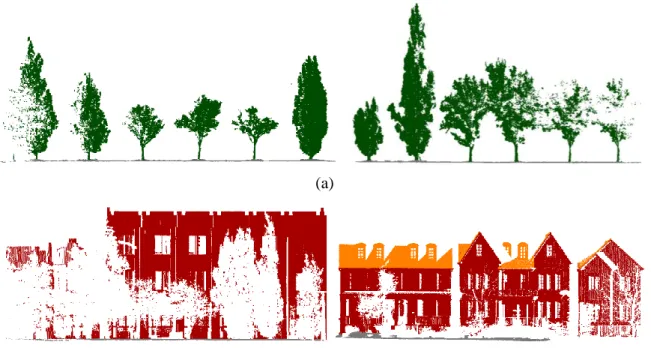
for example, different tree species have different shapes (Figure 1.1(a)) and structures

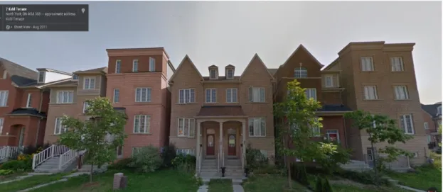
and building at different locations have different architectural styles (Figure 1.1(b)). In

IQmulus & TerraMobilita mobile laser scanning data, pedestrian class can be further

categorized into seven subdivision such as: still pedestrian, walking pedestrian, running

pedestrian, stroller pedestrian, holding pedestrian, leaning pedestrian and other pedestrian

(24)

Figure 1.1: Examples of objects in terrestrial laser scanning data. Color setting:

green-tree; brown-building; orange-roof.

Due to the limit of line-of-sight of static laser scanning, some objects are occluded

by other objects that are closer to the laser scanner, which results in some holes in the

occluded object. It is observed in Figure 1.1(b) that trees are in front of buildings and thus

many tree-shape holes are founded in the building area. Occlusion reduces the

information about the objects of interest and brings problem for further data processing.

The point density varies with the range between laser scanner and objects. The

point density decreases when the distance between the object and the laser scanner

increases. The various point density will make the same type of objects have different

geometric appearance when the distance changes.

(a)

(25)

All of problems mentioned above will cause the problem of feature ambiguity,

which is also called feature overlap. Feature distribution of different classes could

overlap in the feature space, which results in a non-linear separable classification

problem(Lalonde et al., 2005). Building classifiers only relying on these features with

serious ambiguity poses risk of misclassification (Trappenberg and Back, 2000).

A popular solution to solve the problem of feature ambiguity is applying object

context, or context for short, which can be defined as dependencies or correlation among

spatial entities (such as points, lines, or surfaces) in a scene. With context, a spatial entity

is perceived associated with its surrounding neighbors rather than independently.

Classifiers that do not consider context are called local classifier and those considering

context are called context based classifiers. Markov Random Field (MRF) was proposed

by Clifford (1990), and is a commonly used context based model. The MRF model has

been approved to be effective on laser scanning data classification (Anguelov et al., 2005;

Triebel et al., 2006; Munoz et al., 2008; Zhang and Sohn; Häselich et al., 2011). However,

MRF can only maximize the local label homogeneity between adjacent entities, but fails

to capture those relations at global level. For example, MRF can model the relations as

“the building is likely to be neighbor with the building”, but is unable to express interactions between different objects, such as “the building is above the ground but

below the roof”. Therefore, a MRF based method is probably to produce an

over-smoothness (minority objects are misclassified as the class that its surrounding majority

(26)

To avoid the over-smoothness problem, the global object scene layout is usually

considered. The scene layout corresponds to the relative locations of objects in a scene,

and assumes that image (or a point cloud) is not a random collection of independent

pixels (or points), but follows some rules on spatial arrangement. With the prior

knowledge on scene layout, it is expected to estimate what types of objects could be

above or below building, and so on. The scene layout can be modeled as a co-occurrence

matrix, but it is more frequently modeled as data-dependant interaction potential function

in a CRF model. Many achievements has been made on applying scene layout for object

recognition from images (Winn and Shotton, 2006; Heesch and Petrou, 2010; Jahangiri et

al., 2010; Ding et al., 2014). But just a few publications focus on applying scene layout

on TLS data classification. Pu and Vosselman (2009) applied manually defined scene

layout rules on classifying TLS data. Although such rule-based method is easily

implemented and achieved satisfying classification result, but, it cannot cover all the rules

that govern object layout, let alone conditions behind these rules.

All contexts mentioned above, local smoothness and scene layout provide

contextual information on different scales. Each single context contains partial contextual

information, so relying only on a single context could be risky as “part of the evidence is

spent to specify the model” (Leamer, 1978). It is promising to combine all types of contextual information together in one CRF model.

(27)

1.2 Research Objectives

The main objective of this thesis is to develop an automatic, accurate and robust

classification algorithm for TLS data processing. Accordingly, the specific objectives are

as follows:

1. Develop a line-based TLS data classification algorithm. We will explore the

potential of lines as the geometric primitive for TLS data classification. The lines

extraction is based on the “line profiling” nature of laser scanning. Each scan

profile is considered as a stream of sequentially observed laser points, and those

neighboring points that have small range difference were merged into a line. The

line is the highest level geometric primitive that can be extracted from profiling

data, so that the line primitives are expected to be optimal for characterizing street

objects and gaining computational benefits. As line extraction is implemented

within each scan profile, it is also suitable for a real-time point cloud processing.

2. Enhance classification accuracy using multi-range contexts. As mentioned

previously, complex urban scene, appearance variations, occlusions and various

point density with range can result in the problem of features ambiguity. Relying

only on these features with ambiguity, conventional local classifiers cannot

properly identify the boundaries between classes. To improve the classification

performance of local classifier, multi-range (short range and long range) contexts

are introduced. The short range context imposes local smoothness constraint that

neighboring lines are likely to have the same class label. While the long range

(28)

arrangements of objects in the space, both in vertical (“above-below” relation)

and horizontal (“front-behind”) directions. Moreover, local smoothness constraint

is also considered between lines at adjacent scan profiles, which makes lines gain

additional contextual information.

3. Enhance classification accuracy using context propagation. The acquisition of

laser scanning data can be regarded as the process that a set of vertical scan

profiles are sequentially obtained along the azimuth direction. Thus, object can be

viewed as “growing” along the direction that laser scanner sweeps, and so the

class label also can be propagated in the spatial domain. To make the contextual

information propagate from one scan profile to other scan profiles that far away, a

sequential processing can be used. Each time, posterior of the previous

multi-range based classifier is used as association term of the next multi-multi-range based, so

that posterior probability is dynamically updated and confidence gets stronger and

stronger.

1.3 Methodology Overview

In this thesis, we are interested in classifying static terrestrial laser scanning data. The

raw data we get from the laser scanner include 3D coordinates (X, Y, Z), range, azimuth

angle and zenith angle. Line is used as the primitive entity of TLS data classification. The

whole TLS data was firstly split into a set of vertical scan profiles according to azimuth

angle. Points in each scan profile were further segmented into a set of lines based on

(29)

line, including local appearance, circle- based and column-based features. Then the

Principle Component Analysis (Krzanowski, 2000) was applied to reduce the feature

dimension. To validate the effectiveness of line based TLS data classification, both

generative and discriminative classifiers were tested, including Naïve Bayes (Bishop,

2006), Multivariate Gaussian (Bishop, 2006), Gaussian Mixture Model (Bishop, 2006),

K-Nearest Neighbor (Bishop, 2006), Logistic Regression (Menard, S., 2002), Support

Vector Machine (Burges, 1998), Artificial Neural Network (Bendiktsson et al., 1990),

Decision Tree (Quinlan, 1986), and two Decision Tree based ensembles, Random Forest

(Breiman, 2001) and Adaptive Boosting (Freund et al., 1995).

In order to overcome the problem of feature ambiguities in local classifiers,

multi-range contexts along scan profile were used, including short multi-range context that enforces

local smoothness, as well as the long range vertical and horizontal context that provide

priori information of scene-layout compatibility. The three types of adjacent relations of

lines were defined with the assistant of a grid system. At first, the scan profile was

projected into 2D space (XY-Z) and then the 2D space was quantized in a grid along the

Z and XY directions, with cell size of 0.5m by 0.5m. Neighbor searching of a line is

based on neighboring relations of cells. In particular, we adopted an asymmetric

interaction potential to capture directional scene layout (e.g. ground is lower than

building, not vice-versa). To integrate context into a classification problem, Conditional

Random Filed (Lafferty et al., 2001) was used. Finally all the three different contexts are

(30)

effect of different types of contexts and validate the advantage of multi-range context,

three single range CRF models were also constructed.

The maCRF was also extended to across scan profiles, which is called across scan

profile multi-range asymmetric CRF (amaCRF). The amaCRF graph was built on three

consecutive scan profiles; and four types edges are considered, short range, long range

vertical and horizontal, as well as across scan profile edge. To make the contextual

information propagate from one scan profile to other scan profiles that indirectly connect

with it, a sequential processing was used (amaCRF+). Each time, posterior of the

previous amaCRF classifier is used as association term of the next amaCRF, so that

posterior probability is dynamically updated and confidence gets stronger and stronger.

There are two types of parameters in each of the five CRF models: parameters in

each potential term, and parameters weighting the relative influence of potential terms.

Learning all of the parameters simultaneously in each CRF models is still a challenge;

thus, parameter learning was divided into two stages. At first, parameters in association

and each interaction terms were learned individually, following which the weights of

association and interaction terms were learned using Stochastic Gradient Descent

(Vishwanathan et al., 2006). Given learned parameters, the loopy belief propagation (Frey

et al., 1998), a variant of belief propagation (BP), was used for inference; and the final

class label was selected by maxizing node belief.

Finally the proposed classifier was tested on several TLS data collected in York

Village, Toronto. The performance of classification was evaluated both qualitatively and

(31)

precision, recall and F1-score. To track how different types of context affect the

classification result, one representative scan profile was selected for comparative analysis.

In order to examine which classes are sensitive to which type of context, label transition

analysis was analyzed, which is based on comparing label change from local classifier to

CRF model.

To test the whether the function of multi-range context is dependent on

association terms, both output of GMM and SVM were used as association term. To

validate that the algorithm is not only work on a specific scene, another TLS data were

tested, collected at York Blvd, Toronto.

1.4 Outline

Chapter 2: We present literature review on mechanism of terrestrial laser scanning

technology and popular classification methods. Comparison of various classification

methods are discussed, including rule-based methods verses machine learning methods,

generative classifiers verses discriminative classifiers, local classifiers verses context

based graphical models, MRFs verses CRFs. In particular, the information loss

challenges in TLS data classification and potential of scene layout for enhancing

classification performance is discussed.

Chapter 3: At first, data prepossessing for line-based classification will be

introduced, including technique characteristics of the experimental laser scanner, data

collection, data preprocessing, line segment extraction, and feature generation. Principle,

(32)

are presented. Finally, the ten classifiers are tested on TLS data collected at York Village,

and performances of these classifiers are compared.

Chapter 4: We propose a multi-range asymmetric CRF model (maCRF) to

enhance classification performance. Limitation of local classifier is discussed first using

the experimental result of GMM for example. Then three types of object context within

along scan profile are exploited: short range context that enforces local smoothness, as

well as long range vertical and horizontal context that provide priori information of scene

layout compatibility of objects. Three single range CRF models and the integrated

multi-range asymmetric CRF model are presented. The output of GMM is used as association

term of the four CRF models. Performances of the four CRF models are evaluated using

the same experimental data, and compared with the results of GMM classifier.

Chapter 5: The maCRF model is extended from only along scan profile contexts

to the across scan profile context (amaCRF). Furthermore, a sequential knowledge

propagation method (amaCRF+) is proposed to make contextual information propagate

through adjacent scan profiles. To validate that the multi-range context CRF model is not

sensitive to the association term, output of GMM (generative) was replaced with SVM

(discriminative). To validate that the multi-range context CRF model is not sensitive to

dataset, TLS data collected at a different site, York Blvd, was also tested.

(33)

Chapter 2 Background

2.1 Terrestrial Laser Scanning Technology

2.1.1 Laser Scanning Mapping

Since the first laser instrument for distance measurement was invented in 1966, laser

scanning has been the standard for a wide range of applications (Heritage and Large,

2009). LiDAR, which stands for Light Detection and Ranging, is an active remote

sensing technology for detecting the surrounding environment. Laser scanning is an

effective way of capturing surface information of targeted objects. Compared with

traditional surveying and mapping technologies, laser scanning mapping provides

advantages like high accuracy, fast collection and cost-efficiency. It has been widely used

for civil surveying and mapping, such as high-resolution topographic mapping (Kraus

and Pfeifer 1998), various infrastructure modeling (Kim and Sohn, 2010; Shapovalov et

al., 2010) and forest studies (Rutzinger et al., 2008; Vehmas et al, 2009; Zhang and Sohn,

2010) , etc.

A typical laser scanning system consists of a laser scanner, and some additional

onboard equipment for positioning and navigation, such as an onboard Global Position

System (GPS) and Inertial Navigation System (INS) system (Wehr and Lohr, 1999). The

GPS is used to translate laser system coordinates to the global geographic coordinates.

The INS is used to estimate the attitudes of a moving rigid body by measuring the angular

(34)

signal reflected by the surface it encounters. By comparing the sending and reflected

signal, the range between laser scanner and the object of interest can be calculated. To get

the 3D coordinates of objects, the range value needs to be combined with position and

orientation, from GPS and INS respectively. This set of points with coordinates is usually

called “point cloud”.

The ranging technologies using a laser can be classified into two groups: phase

comparison and time pulse method (Shan and Toth, 2009). In the phase comparison

method, the scanning system transmits a continuous wave (CW) of laser radiation. The

ranges between the laser scanner and objects are determined by comparing the

transmitted and received wave patterns. The laser ranging system using a CW is usually

used in terrestrial LiDAR systems aiming to measure relatively short distances. The

drawback of the CW system is that the phase difference between reflected and emitted

signals is measured by comparing them, but the integer number of wavelengths cannot be

determined by the signal difference. It is known as the ambiguity resolution problem,

which is similar to the GPS carrier-phase ambiguity problem. In modern systems, the

problem is solved by making many changes to the wavelength (Shan and Toth, 2009).

Second, ‘time pulse method’ transmits discrete pulses instead of the CW and records time difference between transmitted and reflected pulses to determine the distance for the

round trip (Baltsavias, 1999; Wehr and Lohr, 1999). Usually, when the pulse is reflected

from the specific targets such as grounds, buildings, and trees, the received pulses whose

energy is higher than a predetermined threshold value can be detected. The detected pulse

(35)

which is known as the waveform. Since the speed of light is accurately known, the

accuracy of the laser range is dominantly affected by the quality of the time

measurement.

In the 1980s, NASA launched the first laser altimetry system, called Airborne

Topographic Mapper, while the first commercial airborne LiDAR system was developed

by 1995 at Optech Incorporation, Canada. In recent years, with the continuing

improvement in accuracy and density of laser measurement, more accurate positioning

and navigation system, as well as more advanced solutions for data processing, laser

scanning has showed its potential in surveying and mapping (Vosselman and Maas,

2010).

2.1.2 Introduction of Terrestrial Laser Scanning

A laser scanner put on the platform of an airplane is called an airborne laser scanner

(ALS). Due to rapid, accurate and dense data acquisition, ALS has been widely applied

for DEM modeling (Kraus and Pfeifer 1998), forest inventory investigation (Rutzinger et

al., 2008; Vehmas et al, 2009; Zhang and Sohn, 2010; Kantola et al, 2013), 3D power

line modeling (Kim and Sohn, 2010), 3D city modeling (Shapovalov et al., 2010). There

is an increasing demand for fine 3D urban object modelling, which aims to capture full

geometric details of objects, such as roof, façade, even the interior structure. However,

ALS collects data from the bird’s eye view, and cannot completely cover details at the ground level, like building facades. Therefore, the ground-based terrestrial laser scanning

(TLS) might be able to provide complementary measurements for ALS, by placing the

(36)

surveying accuracy, terrestrial laser scanning is feasible for all kinds of detailed 3D

documentation, such as digital factory, virtual reality, architecture, civic engineering and

culture heritage, plant design and automation systems.

A laser scanner sends out signals toward a specific direction and receives the

reflected signal, so only one point is detected at a time. To capture a broad view, the laser

scanner changes beam emitting direction to sweep through the whole targeted area; laser

beam direction change can be achieved by a system of rotating mirror or rotating the laser

source itself (Vosselman and Maas, 2010). However, due to the limited view of static

laser scanning, the background region is occluded by the foreground objects. This

occlusion prevents the targeted area from being completely scanned, and poses a big

challenge for object recognition.

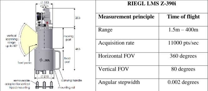
The terrestrial laser scanner used in this research is RIEGL LMS Z-390i, which

uses technology of TOF. RIEGL LMS Z-390i is a long range TLS scanner and its range

varies between 1.5 m to 400 m. The system of rotating mirror is a two-axis system and

allows measurement conducted simultaneously both along vertical and horizontal

direction. The field of view covers 360 degrees horizontally and 80 degrees vertically.

The minimum horizontal and vertical angular stepwidths are both 0.002 degrees. Table

(37)

Table 2.1: Technical specifications of RIEGL LMS Z-390i RIEGL LMS Z-390i

Measurement principle Time of flight

Range 1.5m – 400m

Acquisition rate 11000 pts/sec

Horizontal FOV 360 degrees

Vertical FOV 80 degrees

Angular stepwidth 0.002 degrees

The scanner is controlled by RiSCAN PRO software, which provides complete

data collection services, including sensor configuration, data acquisition, visualization,

and manipulation. Direct measurements for each laser return include range, horizontal

angles, and vertical angles. The RiSCAN PRO software is able to automatically calculate

3D coordinates from these direct measurements. Finally, data collected by the sensor is

transferred to a computer via USB connection.

2.1.3 Terrestrial Laser Scanning Data Classification

With the development of laser scanning and related technology, TLS has been rapidly

adopted for urban street data acquisition. Classification is a necessary step for further

application, but classifying such complex urban street scenes in an automated manner

still remains as a challenging vision task. According to the primitive spatial entity, TLS

data classification can be categorized into point-based classification (Triebel, et al, 2006;

(38)

al., 2010; Hu and Ye, 2013) and surface-based classification (Belton and Lichti, 2007; Pu

and Vosselman, 2009).

As regard the features used for classification, commonly used features include

spectral features and geometric features. Spectral features provide information on

physical properties of objects. Intensity is typical spectral information; it is dependent on

reflectivity and scattering characteristics of object surface (Pfeifer et al., 2007). Imagery

from an attached camera also can provide additional spectral features; it usually needs to

be registered with the point clouds (Forkuo and King, 2004). However, the laser scanner

we used has a problem of outputting intensity, so this research relies purely on geometric

information that is derived from 3D coordinates of point clouds.

Geometric feature can be extracted based only on a single spatial entity (e.g.,

point, line, and surface) without considering its neighborhood. Another type of feature is

neighborhood-based feature, which provides contextual information. The neighborhood

can be selected by searching neighbors in a pre-defined region (Niemeyer, et al., 2012;

Kim and Sohn, 2010), or k nearest neighbors (Munoz et al., 2008; Niemeyer et al., 2011,

Schmidt et al., 2012) are popular methods. Given the neighborhood, geometric features

can be calculated, such as eigenvalue based features (Belton and Lichti, 2006), hough

transformation based features (Kim and Sohn, 2010), point density based features

(Rutzinger et al, 2008), and features based projected 2D space (Weinmann et al., 2013).

When features extraction is done, classifiers can be built based on these features.

There are two primary classification strategies, rule-based classification and machine

(39)

2.1.3.1 Rule Based Classification

Rule based methods usually implement classification by converting prior expert

knowledge to simple “if this, then that” clause (Forlani et al., 2006; Goulette et al., 2006;

Pu and Vosselman, 2009; Lehtomäki et al., 2010; Aijazi et al., 2013). Forlani et al. (2006)

applied a set of hierarchically predefined rules to classify segmented laser scanning data

into bare terrain, building, vegetation, courtyard, and water from ALS data; these rules

were based on geometric and topological properties (e.g., regions exceeding a size of

200000 m2 were classified as terrain). Goulette et al. (2006) detected ground from

vehicle-based TLS data by assuming that ground points correspond to the peak of

histogram of vertical coordinates. After removing ground, building and tree were then

recognized by detecting peaks in the histogram of horizontal coordinates. Pu and

Vosselman (2009) manually defined classification rules based on point segments’

characteristics, such as size, position, orientation, and topological relations. In Lehtomäki

et al. (2010), vertical pole-like objects were detected by fitting circle and arc models from

horizontal slices of point clouds. Candidate circles can be classified as pole only if they

fulfil all requirements on length, shape, orientation, etc. Authors claimed that thresholds

they used need to be adjusted according to the real data. Aijazi et al. (2013) classified

super-voxels into ground and other five non-ground objects using both geometrical

models (e.g., roads represent a low flat plane, while the buildings are represented as large

vertical blocks) and predefined rules (e.g., barycenters of tree and vegetation are greater

(40)

These rule based methods have many advantages: they are easily designed and

implemented; the inference rules can be modified and updated according to real data;

they do not require labeled training data. However, classification performance of rule

based methods is highly dependent on the choice of features and thresholds; thus rule

makers should have sufficient prior knowledge about the target classes. Unfortunately,

rule makers often cannot discover all the rules that govern objects, let alone the various

conditions behind these rules. In contrast, machine learning is able to learn classification

rules automatically from labeled data; they also can be implemented and updated easily.

2.1.3.2 Machine Learning

Machine learning based laser scanning classification has attracted more and more

attention over recent years. Supervised classification method is one of the most popular

machine learning strategies and has been widely applied for object recognition.

Supervised methods learn statistical rules automatically from labeled training data, and

then generalize these rules on unseen data (Kotsiantis, 2007). Supervised methods can be

categorized into “generative classifiers” and “discriminative classifiers”. Generative

classifiers model joint distributions of class label and features and provide rigorous

framework to combine prior knowledge and observed data. Generative classifiers can

freely generate new labeled instances according to these joint distributions. Many

generative classifiers have been used for laser scanning data classification, such as Naïve

Bayes (Premebida et al., 2009; Posner et al., 2009), Gaussian Mixture Model (Charaniya

(41)

The Naïve Bayes classifier makes the assumption that each attribute of the feature

vector is independent, and the likelihood is modeled as the product of class conditional

probability of each attribute (Premebida et al., 2009), which is often modeled using

Gaussian distribution. However, the class conditional probability is usually very complex,

so single Gaussian distribution cannot fit it well. An alternative is Gaussian Mixture

Model (GMM), which decomposes a distribution using linear combination of several

Gaussian distributions (Charaniya et al., 2004; Lalonde et al., 2006). Parameters in the

GMM are usually estimated using the classic Expectation Maximization (EM) algorithm

(Dempster et al., 1977). If given sufficient expert knowledge on the classification

problem domain, Bayesian Network is a proper choice; it models direct dependencies

and local distributions between variables (Brunn and Weidner, 1997).

On the other hand, the “discriminative classifiers” are concerned with finding the

boundaries between different classes, and directly model the posterior probability.

Discriminative classifiers, such as k-Nearest Neighbour (Vehmas et al., 2009;

Golovinskiy et al., 2009), Logistic Regression (Vehmas et al., 2009; Saxena et al., 2008),

Support Vector Machine (Posner et al., 2007; Nüchter and Hertzberg, 2008; Golovinskiy

et al., 2009; Himmelsbach et al., 2009; Brodu and Lague; 2012), Decision tree

(Matikainen et al, 2007), Neural Network (Nguyen et al., 2005; Priestnall et al., 2000;

Prokhorov, 2009) have been applied for laser scanning data classification.

K-nearest neighbour is a non-parametric method and assigns to a new instance

with the majority class of its k nearest training samples (Cover and Hart, 1967). Nearest

(42)

data (Vehmas et al., 2009), and choice of the number of neighbors (Golovinskiy et al.,

2009). Logistic regression is a basic parametric method for binary classification and uses

logistic transformation to make the relationship between the posterior probability and

linear combination of features (Hosmer and Lemeshow, 2004; Saxena et al., 2008). More

recently, Support Vector Machines (SVM) attracts more attention as an alternative for

laser scanning data classification (Posner et al., 2007; Nüchter and Hertzberg, 2008;

Golovinskiy et al., 2009; Himmelsbach et al., 2009; Brodu and Lague; 2012).The

principle of SVM is maximizing the margin, which is defined as the shortest distance

from the separating hyperplane to the closest positive (negative) example (Burges, 1998).

However, the linear decision boundary found by the classic linear SVM has risk of

misclassification if the dataset is not linearly separable, thus kernel function is often used

to find a non-linear separating hyperplane by mapping original features into a new

high-dimension space (Wang, 2005). An Artificial Neural Networks (ANN) is a computational

model inspired by the mechanism of the human neurons. It is comprised of densely

interconnected adaptive simple processing elements (called artificial neurons or nodes),

which are capable of performing massively parallel computations for data processing and

knowledge representation. Variants of ANN, such as Hopfield Neural Network (HNN)

and Recurrent Neural Network (RNN) have shown its potential in classifying laser

scanning data (Basheer and Hajmeer, 2000; Prokhorov, 2009).

Recently, more attention has been turned to ensemble learning (Drucker et al,

1994), which increase the accuracy of single classifier by combining results of some

(43)

categorized into bagging and boosting. In Breiman (1996), the concept of bootstrap

aggregation was introduced, and the strategy using bootstrap to generate weak classifiers

is called bagging. Random forest is a typical bagging method that constructs a set of

decision trees using bootstrap. In addition to resampling, candidate features for splitting

at each node are also randomly chosen, which increases independency of trees (Liaw and

Wiener, 2002). Random forest has achieved good prediction result in urban scene

classification (Chehata et al., 2009), power line corridor recognition (Kim and Sohn,

2010), forest type classification (Kantola et al., 2013) from laser scanning data. Instead of

randomly sampling training data and combining classifiers with equal vote as the bagging

method, the boosting method uses a weighted sample to focus learning on those samples

that misclassified by previous weak classifiers, and finally combines results of weak

classifiers using weighted vote (Freund et al., 1999). The adaptive boosting (Adaboost) is

a typical boosting model, and has been applied to classify laser scanning data (Lodha et

al., 2007).

2.2 Context Based Object Recognition

The machine learning based methods mentioned in section 2.1 are called local classifier

because they only use appearance features, without considering relations between objects.

Appearance variation, occlusion, various point density with range, all of which cause the

problem of feature ambiguity. Relying only on these features with ambiguity, local

classifiers have risk of misclassification.

Contextual information, or context for short, has been proved to be able to remove

(44)

(1993) defined the context as any and all information that may influence the way a scene

and the objects within it are perceived. Therefore, data collected for the same object using

different sensors, time of data collection, attributes of local region, and global scene

layout of objects are all parts of context. The context can be defined at visual perception

level and objective statistical level. Visual perception is the ability to interpret the

surrounding environment by processing information that is contained in visible light;

illusions (such as the Muller-Lyer illusion) and Stroop phenomenon are typical

modalities of visual perceptual context (Toussaint, 1978). Meanwhile, the statistical

context is defined under an elegant probabilistic framework (Song, 1999). In this

research, we utilized the statistical method to model context.

2.2.1 Object Context

Object context in this research is indicates dependencies or correlations among entities

(line) in a scene. With context, a line is perceived associated with its surrounding

neighbors rather than independently. Galleguillos and Belongie (2010) categorized the

statistical context used for object recognition into three types: semantic (probability),

spatial (position) and scale (size).

Semantic context indicates the occurrence probability that an object can be found

in a specific scene but not others. Early studies on semantic context mainly focused on

manually-made rules, but current research prefers to extract context automatically from

labeled training data. The symmetric, nonnegative co-occurrence matrix is a typical form

(45)

Rabinovich et al. (2007) used this type of co-occurrence matrix among segment labels to

enhance classification performance. Soh and Tsatsoulis (1999) defined the gray-level

spatial dependence over pixels using a gray-level co-occurrence matrix (GLCM), where

each entry P(i,j) of the GLCM corresponds with the number of co-occurrence of the pair

of grey level i and j at a distance of d.

Spatial context specifies the likelihood of finding an object at some position. The

spatial context can be defined based on absolute position (Shotton et al., 2006; Shotton et

al., 2009; Bo et al., 2011; Liu et al., 2011; Zitnick et al., 2013) or relative position (Gould

et al., 2013; Zitnick et al., 2013) in a scene. Shotton et al. (2006) encoded the probability

of a class occurs at the specific location in the image as the form of a look-up table.

Gould et al. (2013) used non-parametric relative location maps over super-pixels as a

global feature, which not only allows modeling simple relative location relations (above,

beside, or enclosed), but also complex relationships, such as both sky and car are found

above road, but car tends to be much closer than sky. Zitnick et al. (2013) incorporated

both absolute location prior and relative location prior in their probabilistic model.

Scale context refers to prior information about the most likely sizes at which

objects might appear in the scene (Torralba, 2003). Meta-data (e.g. position, orientation,

geometric horizon, and map) of cameras is able to generate hypothesis about the scene in

which object’s configurations are consistent with a global context (Strat and Fischler, 1991). Scale context is the hardest relation to access, since it requires more detailed

(46)

Actually, the boundaries between different types of context are not strictly defined.

Most of publication we reviewed above perhaps used one or two explicit types of context.

A critical contribution of this research is exploiting scene layout of object to improve

classification; the scene layout can be sematic context or spatial context. While images

have scaling problem because object size varies with the focal length, the TLS scanner

captures direct 3D coordinate of target objects; thus, the scaling context is of no benefit

and was not considered.

2.2.2 Scene Layout Prior

The scene layout corresponds to the relative locations of objects in a scene. An image (or

a point cloud) is not a random collection of independent pixels (or points), but follows

some rules on spatial arrangement. The spatial arrangement of objects in urban

environment is rather clear and strict, e.g. roof is on the top of building facade, and

building is behind of tree. With the prior knowledge on scene layout, it is expect to

estimate what types of objects could be above or below building, and so on.

Many achievements have been made on applying scene layout for object

recognition from images (Winn and Shotton, 2006; Heesch and Petrou, 2010; Jahangiri et

al., 2010; Ding et al., 2014). Winn and Shotton (2006) modeled scene layout

(above/bellow/left/right) over pixels using asymmetric pairwise potential. In Gould et al.

(2008), layout of objects was modeled as relative location probability maps over pixels,

which were based on the first-stage classification using appearance-based feature; and the

(47)

interested in modeling the probability distribution over labels for a segmented region

given labels of its six local neighboring regions: above, bellow, left, right, as well as

regions containing and being contained by the current region. Jahangiri et al. (2010)

incorporated five different scene layout relations between segmented region pairs in one

probabilistic model, including relative vertical and horizontal orientation, containment

relation, and the ratio of width and height. In Desai et al. (2011), an image was

represented as a collection of overlapping windows at multiple scales, and spatial relation

between these windows was considered, such as above, below, overlapping, next-to, near,

and far. Label layout filter (LLF) was proposed by Ding et al. (2014) to model the class

distribution behavior and visual context appearance of labels over multi-scale segmented

regions, such as location distribution of each class in the image, or the relative distance

and orientation between two classes. The LLF combines label compatibility, spatial

closeness (distance), and feature similarity on all pairs of pixels from the image scene in

one potential term in forms of appearance kernel and smoothness kernel.

However, not too many was done on applying scene-layout to classify laser point

cloud. Pu and Vosselman (2009) manually defined object’s layout based on size,

position, orientation, etc., from human knowledge and then apply these predefined rules

on classifying TLS data. As it is mentioned above, although such rule based method is

easily implemented and achieved satisfying classification result, it cannot cover all the

rules that govern object layout, let alone conditions behind these rules. Instead, we used

(48)

In this research, the scene layout specifies the relative location of lines in both the

vertical and horizontal directions. The vertical scene layout was considered an

“above-below” relation, such as building is bellow roof but above the pedestrian road. The

horizontal scene layout was modeled as a “front-behind” relation, with respect to the

distance between lines and laser scanner center, such as tree is in front of building, but

behind of vehicle road.

2.3 Probabilistic Graphical Model

There exist two methods to utilize contextual information in a classification, contextual

features and contextual classifiers. Contextual features are usually derived from a local or

global neighborhood surrounding the interest region that is being analyzed (Haralick et

al., 2013). Contextual features could be extracted directly from unlabeled data (Kim and

Sohn, 2010; Niemeyer, et al., 2012), or based on an initial classification result that relies

only on appearance features (Gould et al., 2008; Jahangiri et al., 2010). Contextual

features are finally combined with appearance features to make a final decision using any

classifier. Instead of modeling contextual information as features, contextual classifiers

incorporate contextual information directly into a probabilistic graphical model.

2.3.1 Probabilistic Graphical Model

Probabilistic graphical model, or graphical model in short, gives a multivariate statistical

modeling based on both the graph theory and probability theory (Koller and Friedman,

2009). By considering dependency of variables, the graphical model greatly simplifies

Line Based Multi-Range Asymmetric Conditional Random Field For Terrestrial Laser Scanning Data Classification